| Issue |
A&A
Volume 649, May 2021
|
|
|---|---|---|
| Article Number | A114 | |
| Number of page(s) | 21 | |
| Section | Stellar structure and evolution | |
| DOI | https://doi.org/10.1051/0004-6361/202038357 | |
| Published online | 26 May 2021 | |
Progenitors of low-mass binary black-hole mergers in the isolated binary evolution scenario
1
AIM, CEA, CNRS, Université Paris-Saclay, Université de Paris, 91191 Gif-sur-Yvette, France
e-mail: This email address is being protected from spambots. You need JavaScript enabled to view it.
2
Kapteyn Astronomical Institute, University of Groningen, PO Box 800 9700 AV, Groningen, The Netherlands
3
Instituto Argentino de Radioastronomía, Universidad Nacional de La Plata, 1900 La Plata, Argentina
4
Université de Paris, CNRS, Astroparticule et Cosmologie, 75013 Paris, France
Received:
6
May
2020
Accepted:
2
March
2021
Abstract
Context. The formation history, progenitor properties, and expected rates of the binary black holes discovered by the LIGO-Virgo collaboration via the gravitational-wave emission during their coalescence are a topic of active research.
Aims. We aim to study the progenitor properties and expected rates of the two lowest-mass binary black hole mergers, GW151226 and GW170608, detected within the first two Advanced LIGO-Virgo observing runs, in the context of the classical isolated binary-evolution scenario.
Methods. We used the publicly available 1D-hydrodynamic stellar-evolution code MESA, which we adapted to include the black-hole formation and the unstable mass transfer developed during the so-called common-envelope phase. Using more than 60 000 binary simulations, we explored a wide parameter space for initial stellar masses, separations, metallicities, and mass-transfer efficiencies. We obtained the expected distributions for the chirp mass, mass ratio, and merger time delay by accounting for the initial stellar binary distributions. We predicted the expected merger rates and compared them with those of the detected gravitational-wave events. We studied the dependence of our predictions with respect to the (as yet) unconstrained parameters inherent to binary stellar evolution.
Results. Our simulations for both events show that while the progenitors we obtained are compatible over the entire range of explored metallicities, they show a strong dependence on the initial masses of the stars, according to stellar winds. All the progenitors we found follow a similar evolutionary path, starting from binaries with initial separations in the 30−200 R⊙ range experiencing a stable mass transfer interaction before the formation of the first black hole, followed by a second unstable mass-transfer episode leading to a common-envelope ejection that occurs either when the secondary star crosses the Hertzsprung gap or when it is burning He in its core. The common-envelope phase plays a fundamental role in the considered low-mass range: only progenitors experiencing such an unstable mass-transfer phase are able to merge in less than a Hubble time.
Conclusions. We find integrated merger-rate densities in the range 0.2–5.0 yr−1 Gpc−3 in the Local Universe for the highest mass-transfer efficiencies explored here. The highest rate densities lead to detection rates of 1.2–3.3 yr−1, which are compatible with the observed rates. The common-envelope efficiency αCE has a strong impact on the progenitor populations. A high-efficiency scenario with αCE = 2.0 is favoured when comparing the expected rates with the observations.
Key words: gravitational waves / binaries: general / stars: evolution / stars: black holes
Fellow of CONICET.
© ESO 2021
1. Introduction
In 2015, the Advanced LIGO (LIGO Scientific Collaboration 2015) and Advanced Virgo (Acernese et al. 2015) Collaboration (LVC) began a series of observation runs. During both the O1 (12 September 2015–19 January 2016) and O2 (30 November 2016–25 August 2017) observation runs, a total of 11 gravitational wave (GW) events were observed. Ten of these events involved the detection of signals from the merger of a binary black hole (BBH, Abbott et al. 2019a) and one corresponded to the merger of two neutron stars (Abbott et al. 2017a, GW170817).
While the detected BBHs are mainly dominated by high-mass components (M ≳ 35 M⊙), two detections in particular, GW151226 (Abbott et al. 2016a) and GW170608 (Abbott et al. 2017b), are shown to be low-mass systems having BH masses consistent with those found in X-ray binaries (i.e., M ≲ 20 M⊙). Despite the fact that all these events could belong to the same population (Abbott et al. 2019b), the existence and abundance of these objects have triggered questions regarding their formation history. Several scenarios have been proposed in the literature, including the isolated binary evolution (our main focus here, Bethe & Brown 1998; Mandel & de Mink 2016; Tauris et al. 2017) and the dynamical formation channels (Portegies Zwart & McMillan 2000; Bae et al. 2014; Rodriguez et al. 2016).
In the dynamical formation scenario, BBHs are produced by three-body encounters in stellar clusters. In the chemically homogeneous evolutionary channel, compact BBHs are formed from rapidly rotating stars in near contact binaries that experience efficient internal mixing. It is estimated that dynamical encounters in globular clusters contributed to less than a few percent of all observed events (Bae et al. 2014; Rodriguez et al. 2016), while BBH rates in open and young star clusters can be an order of magnitude higher (Di Carlo et al. 2019; Kumamoto et al. 2020). On the other hand, the chemically homogeneous scenario is not able to produce a BBH in the low-mass range, with M ≲ 10 M⊙ (Marchant et al. 2016). In this study, we concentrate on the classical isolated binary evolution scenario where the formation of the ultra-compact binary leading to the BBH merger is driven through an unstable mass-transfer phase where a common-envelope (CE) is ejected (Ivanova et al. 2013; Kruckow et al. 2016).
Our main goal is to study the progenitor population of the lightest BBHs detected by Advanced LIGO and Advanced Virgo during their first two science runs, namely, O1 and O2, and its dependence on the uncertainties intrinsically related to binary stellar evolution, such as the accretion efficiency during a stable mass-transfer phase, efficiency of the CE ejection, impact of metallicity, and the evolution of merger rates with redshift.
This sort of study has typically been performed following a binary population synthesis approach using several different numerical codes (Lipunov et al. 1997; Belczynski et al. 2002; Voss & Tauris 2003; Belczynski et al. 2016; Eldridge & Stanway 2016; Stevenson et al. 2017; Kruckow et al. 2018; Spera et al. 2019). In this work, we perform detailed numerical stellar simulations of the binary systems, using the 1D-hydrodynamic stellar-evolution code MESA1. Such a treatment, which has recently been in development (see, for instance, Marchant et al. 2017), allows for an accurate modelling of the mass-transfer between the binary components that holds consequences for the final BH masses before the merger. However, the method is computationally expensive, which is the reason it is usually not considered in standard binary population studies. Our simulations incorporate the evolution during the CE phase, which plays a fundamental role in the low-mass BBH range considered here.
The paper is organised as follows. We first describe the binary stellar evolution using MESA in Sect. 2. We then focus on the results for GW170608 and GW151226 in Sect. 3. We report on the population-weighted results in Sect. 4 and give the projected merger and gravitational-wave event rates in Sect. 5. Finally, we discuss the results in Sect. 6 and provide our summary and conclusions in Sect. 7.
2. Binary stellar evolution using MESA
Here, we present models of stellar-binary systems that evolve starting from zero-age main sequence (ZAMS), to the formation of binary black holes (BBH) and their final merger through the emission of gravitational waves (GW). We made use of the publicly available stellar evolution code, MESA (Paxton et al. 2010, 2011, 2013, 2018, 2019), which we modified2 to include a treatment for the common-envelope (CE) phase and BH formation, in addition to properly merging, in a single run, the three evolutionary stages involved in this problem, that is: a binary of massive stars, massive stellar evolution and BH formation, and the formation of a binary BH.
2.1. Microphysics, nuclear networks, and stellar winds
Our simulations were computed using MESA version 10398. We used CO-enhanced opacity tables from the OPAL project (Iglesias & Rogers 1993, 1996). Convection was modelled following the standard mixing-length theory (MLT, Böhm-Vitense 1958) adopting a mixing-length parameter αMLT = 1.5. Convective regions were determined using the Ledoux criterion. In the late evolutionary stages of massive stars, the convective velocities in certain regions of the convective envelope can approach the speed of sound, running out of the domain of applicability of the MLT. For these regions, we used an MLT++ treatment (Paxton et al. 2013) that reduces the super-adiabaticity. Semi-convection is included according to the diffusive approach presented in Langer et al. (1983), which depends on an efficiency parameter that we assume to be αSC = 1.0. We also include a convective-core overshooting during H burning extending the core radius given by the Ledoux criterion by 0.335 of the pressure-scale height (HP, Brott et al. 2011). When mass is transferred from one star to its companion, the material accreted by the accretor may have a mean molecular weight higher than its outer layers. This leads to an unstable situation that induces a thermohaline mixing (Kippenhahn et al. 1980), which is factored in by adopting αth = 1.0. In this work, we only consider non-rotating stars, hence, we ignore the effects that tidal interactions may have on internal rotation and mixing and their impact on final BH masses (Heger et al. 2000).
We used standard thermonuclear reaction networks provided by MESA: basic.net for the hydrogen and helium burning phases, and switched during run time to co_burn.net for the carbon burning phase. Furthermore, stellar winds were modelled using mass-loss rates depending on effective temperatures and surface H mass fraction (Xs). When Teff > 104 K, for Xs > = 0.4, we used the prescription from Vink et al. (2001), while for Xs < 0.4 we applied that of Nugis & Lamers (2000). When Teff < 104 K, we adopted the prescription from de Jager et al. (1988).
2.2. From stellar binaries to binary black holes
We modelled stellar binaries and their interactions using the MESAbinary module from MESA. Our simulations start when both stars with masses Mi, 1 and Mi, 2 are at the zero-age main sequence (ZAMS), in circular orbits, at a certain initial separation, ai.
The mass-exchange between the two binary components was modelled as follows. To determine which star is the donor and which is the accretor, the atmospheric transfer (MT) rates of both stars was compared according to Ritter (1988). When one of the stars overfilled its Roche lobe (RLO), we applied an implicit MT scheme to obtain the MT rate (ṀRLOF) at each step. The MT stability was controlled as described in Sect. 2.4.
The accretion efficiency, ϵ, is assumed to remain constant throughout the entire evolution and only considers the mass lost through an isotropic wind in the vicinity of the accretor. Assuming no mass loss from either direct fast winds or a circumbinary co-planar toroid, the efficiency of MT (ϵ = 1 − β) is defined through the β parameter from MESAbinary, which is equal to the fraction of transferred mass that is isotropically lost with the angular momentum of the accretor. Hence, ϵ = 0 indicates a fully inefficient mass transfer (i.e., no accretion).
Once the first BH is formed in the system, we use the point mass approximation from MESAbinary and we limit the accretion onto the compact object to a factor of the Eddington rate ṀEdd,BH = 4πGMBH/ηκdonor, where G is the gravitational constant, κdonor is the opacity of the donor star at its surface and η is the radiation efficiency of the BH, which we set to 1%, implying super-Eddington accretion. The change in the orbital angular momentum is inferred from the effects of mass loss in the binary (MT and stellar winds). In the case of a second BH forming, thus leading to a BBH, the time to merger, tmerger, is estimated from Peters (1964), based on the component masses (MBH), along with their mutual separation and eccentricity.
2.3. Black hole formation
When a non-degenerate star completes the carbon core burning phase, its evolution is stopped as the binary parameters will not change appreciably during the later evolutionary stages due to their short duration (Tauris & van den Heuvel 2006). The BH formation is modelled according to Fryer et al. (2012). Given the actual CO core mass, and the expected BH remnant mass obtained by the ‘delayed’ collapse prescription, we update the orbital parameters of the binary immediately after BH formation, following Bhattacharya & van den Heuvel (1991):
 (1)
(1)
where
 (2)
(2)
At this point, we also check for disruption at BH formation, given by epost-SN > 1. In this calculation, we neglect any interaction with the binary companion and do not consider asymmetric kicks (for a discussion on the impact of asymmetric kicks onto our results, see Appendix E).
2.4. Common-envelope phase
2.4.1. Definition
A common-envelope (CE) phase occurs when the MT becomes unstable. The stability of the MT in binary systems is usually understood in terms of the reaction of the binary components to mass accretion or loss (Soberman et al. 1997). Binary population synthesis (BPS) codes generally associate the MT stability to the binary mass ratio at the onset of the MT phase. If this ratio is above some limit, then the MT is considered unstable, thus typically leading to a CE phase.
However, this assumption was recently revised in Pavlovskii & Ivanova (2015) and Pavlovskii et al. (2017), showing that the mass ratio condition is not sufficient, nor necessary, to predict the outcome of the MT phase. In these papers, based on numerical stellar evolution, the authors show that binaries with mass ratio3q = m2/m1 as low as 0.13 experience a stable MT phase, which stands in contradiction to the findings of earlier works (e.g., Belczynski et al. 2008).
In this work, we assume the MT to be unstable during RLO, when the MT rate exceeds a certain value that we fix to the Eddington limit of the donor, ṀEdd = 4πcR/κ, where R is the stellar radius and c is the speed of light. When the binary consists of two non-degenerate stars, we also consider unstable MT if the MT rate is higher than the Eddington limit of the accretor. In our simulations, these MT rates are on the order of ∼10−2 M⊙ yr−1, which is consistent with the value assumed by Quast et al. (2019) for unstable MT. In contrast to population synthesis codes, MESA allows us to calculate the MT rate at each evolutionary time step. It is thus possible to continuously verify these conditions, even when the binary goes through a RLO phase. Additionally, this allows us to detect late phases of unstable MT rates in the case of long and initially stable RLO phases.
When any of the above conditions are met, a so-called CE phase is triggered. During this phase, the donor star engulfs its companion, while the accretor in-spirals inside the envelope of the donor. A successful envelope ejection may occur on a dynamical timescale (Podsiadlowski 1964). The CE phase plays a crucial role in reducing the separation between two stars, or between a star and a BH, in a binary system, by a factor of 10–100 (Tauris et al. 2017), thus producing ‘ultra-compact’ BBHs. This is fundamental since no BBH is expected to merge in less than the Hubble time when the post-CE system is not ultra-compact in nature in the case when no asymmetric kicks are considered.
2.4.2. Numerical implementation
In order to implement a numerical treatment for the CE phase within MESA, we use the so-called energy formalism (Webbink 1984; de Kool 1990). According to this formalism, the main energy source needed to eject the stellar envelope is provided by the orbital energy reservoir and, thus, by the in-spiral of the companion. Changes in these two quantities are related by a free parameter αCE representing the fraction of the orbital energy deposited as kinetic energy of the envelope components:
 (3)
(3)
where ΔEbind is the change in the binding energy of the donor star envelope, while ΔEorb represents the released orbital energy throughout the in-spiral, and αCE is the CE efficiency that we assume to be fixed throughout the entire CE phase. Here, Ebind is given by
 (4)
(4)
which includes both the gravitational binding energy and the specific internal energy of the envelope. The latter has an additional term associated to the recombination energy of available H and He, which is known to contribute to the ejection of the envelope (Ivanova et al. 2015; Nandez et al. 2015; Kruckow et al. 2016).
Given an unstable MT rate Ṁ, during the time step Δt, the donor losses a mass ΔM = ṀΔt from its outer layer, changing its envelope binding energy by ΔEbind, and, consequently, the orbital energy by ΔEorb, which naturally leads to the spiral-in of the binary. For reasons of numerical stability, once a CE phase is triggered, during a fixed amount of time (which we set to 10 yr), we linearly increase the MT rate up to a fixed maximum value (that we set to 10−1 M⊙ yr−1 throughout this work), we assume that BH mass grow is negligible during this relatively short episode and, thus, we turn off mass accretion onto the companion (MacLeod & Ramirez-Ruiz 2015; De et al. 2020). In Belczynski et al. (2020), the authors argue that recent calculations show that the accretion rates onto compact objects in CE inspiral can be reduced even by a factor of ∼100 with respect to Bondi–Hoyle accretion when the structure of the envelope is taken into account. Moreover, for most density gradients considered by MacLeod et al. (2017), the accretion rate is well below 10% of Bondi–Hoyle accretion rate. Based on these findings, Belczynski et al. (2020) conclude that BHs of ∼30 M⊙ accrete ∼0.5 M⊙ in a typical CE event. In our case, considering BHs of ∼10 M⊙ would lead to an even lower mass accretion during a CE, which is well within the uncertainties of the BH masses in the considered GW events (see Sect. 3).
Once the maximum value for the MT rate is reached, we keep that value constant until the donor star detaches, that is, its radius becomes smaller than its corresponding Roche lobe, or until the merger of the two stars becomes unavoidable, that is, the envelope could not be successfully ejected, leading to a single star or a so-called Thorne–Zytkow object (TZO, Thorne & Zytkow 1977). In this latter case, the evolution is stopped as it would not lead to a BBH4. In the former case, when reaching the detach condition, the mass transfer rate ṀRLOF is linearly decreased, as a fraction of the radius of the lobe, down to the mass loss Ṁth obtained at thermal equilibrium. For those surviving binaries, the donor star becomes an almost naked core, with a tiny envelope rich in H, and with a close companion. The evolution then returns to the standard MESA workflow, allowing for a new stable RLO phase to start.
2.5. MESA runs
As our main goal is to study the progenitor population of the lightest BBHs detected by the LVC during the O1/O2 runs, we explore a wide range of metallicities, that is, Z = 0.0001, 0.001, 0.004, 0.007, and 0.015, which, in principle, can lead to BHs in the mass range of interest. In addition, in order to study the dependence of our results on the poorly-known MT efficiency, we cover a wide range for this parameter with four different values: ϵ = 0.6, 0.4, 0.2 and 0.0, going from efficient to fully inefficient regimes. For each pair of Z and ϵ values, we computed a 3D grid in the parameter space formed by the initial masses (Mi, 1, Mi, 2) and the binary initial separation (ai).
As a first approach, we fixed5αCE = 2.0 and explored a wide range of initial separations that lead to interacting binaries, from 30−4000 R⊙ with relatively large logarithmic step of 0.03 dex. In this initial inspection, we found binaries that went through a CE phase when the first BH was formed for systems with ai < 500 R⊙. Once the broad parameter space was understood, we focussed our searches on this evolutionary channel, but exploring wider ranges of masses, according to metallicity, and lowering the grid spacing in ai to 0.02 dex, for values below 500 R⊙, in order to constrain the regions containing actual solutions, which we call ‘target regions’.
As each MESA simulation is computationally expensive, from this point onwards, we set up a strategy to concentrate our runs on the regions that lead to BBHs with masses in the range of interest, avoiding the calculation of binary systems leading to too light or too heavy chirp masses, as well as avoiding systems that did not display strong interaction (high MT rates) and thus led to extremely long merging times. These ranges depend mainly on Z, but also on ϵ. Thus, for each parameter combination, our runs were set up to cover different ranges, in an iterative fashion, until the target regions were finally bounded.
In order to explore the dependence of our results on the CE efficiency, we ran another set of simulations with αCE = 1.0. In this case, we only ran those simulations for which we already had found a CE trigger and chirp masses in the range of interest. Since the density of CE survivals significantly decreases for this efficiency, due to a natural increase in CE mergers, we decided to increase the grid resolution to ΔM = 1 M⊙ and 0.01 dex in the logarithmic grid of ai, and we proceeded to run the 26 first neighbours in the refined grid for each CE survival of the initial runs. After this step, we proceeded in an iterative manner surrounding the next family of survivals and so on until the process converged.
In Table 1 we summarise the 66 632 simulations computed using our MESA-based numerical code for each MT efficiency ϵ and CE efficiency αCE explored. Full details of the parameter space explored for this work are presented in Appendix A and a full example of a typical MESA simulation leading to a BBH formation after a CE phase is shown in Appendix B.
Number of MESA runs performed for this work.
3. Results for GW 151226 and GW 170608
The response of detectors such as Advanced LIGO and Advanced Virgo to a GW compact binary coalescence depends not only on the distance and relative orientation of the GW source to the detector, but also on the intrinsic binary properties – the most important being the chirp mass (ℳchirp), which affects the phase evolution of gravitational waveform (Finn 1996) and is defined as, ℳchirp = μ3/5M2/5, where μ = MBH, 1 MBH, 2/(MBH, 1 + MBH, 2) is the reduced mass and M = MBH, 1 + MBH, 2 the total mass of the BBH.
GW detections can be used to infer measurements of the redshifted chirp mass in the detector frame, that is,  . In order to estimate ℳchirp in the source frame and, hence, to be able to make a comparison with our theoretical results, the binary masses have to be un-redshifted. Unfortunately, while a direct measurement of the luminosity distance can be made from an inspiral event, without an electromagnetic counterpart, a cosmological model has to be assumed to extract the redshift of the source. For this work, we used a flat ΛCDM model with H0 = 70 km s−1 and TCMB = 2.725 K and the astropy.cosmology package (Astropy Collaboration 2013, 2018) to estimate the masses of the lowest-mass BBHs detected by Advanced LIGO-Virgo in O1/O2 runs (Abbott et al. 2019a). We found
  and
and  for GW151226 and
  and
and  for GW170608, respectively, in their 100% confidence intervals (C.I.).
Throughout this work we consider a certain binary model to be a possible progenitor that is compatible with any of the GW events under study if its ℳchirp and qBBH lays within the 100% C.I. of the corresponding GW event and if it has a merger time delay (tmerger) shorter than the Hubble time (τHubble = 13.46 Gyr, under our cosmological assumptions).
3.1. Parameter space and target regions
We used the models and method described in Sect. 2 to find the target region in the 3D parameter space associated with each GW event for each metallicity and the MT and CE efficiencies.
Figure 1 shows the solution regions for GW151226 and GW170608 obtained with αCE = 2.0, along with their merger time delay. In general, more massive progenitors are needed to explain GW151226 than GW170608 in each individual case, in agreement with their final BH masses. Higher metallicities require increasingly massive stars in order to obtain progenitors of both GW events, which is a direct consequence of the dependence of stellar winds on the metallicity content (see e.g., Kudritzki & Puls 2000). We find that this effect is independent of the MT efficiency. For all metallicities explored at the higher MT efficiencies, ϵ ≥ 0.4, we find progenitors compatible with both GW events, while in the ϵ = 0.2 MT regime, we find that only binaries with Z ≤ 0.007 are capable of becoming actual progenitors. This is because in the ϵ = 0.2 and Z = 0.015 case, the BBHs that merge within a Hubble time have chirp masses below the lower boundaries given by Abbott et al. (2019a) for the least massive BBHs. Furthermore, no compatible progenitors are found for the fully inefficient MT scenario (i.e., ϵ = 0).
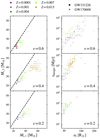 |
Fig. 1. Target regions of the parameter space for GW151226 (square markers) and GW170608 (cross markers) for models with αCE = 2.0. Left panels: progenitor initial masses (Mi, 1 > Mi, 2). Right panels: merger time delay (tmerge) against initial binary separation (ai). Panels from top to bottom correspond to each set of efficiencies: ϵ = 0.6, 0.4, 0.2. Dashed lines indicate equal progenitor masses. |
Another interesting feature in Fig. 1 is that at low metallicities, when Z ≤ 0.004, and high MT efficiencies, ϵ ≥ 0.4, binaries with similar initial masses are admissible progenitors. Efficient accretion favours the growth of a convective core in the accreting star, which in our case is typically located on the main-sequence (MS), leading to a rejuvenation (Braun & Langer 1995; Dray & Tout 2007) and, thus, a longer duration of the core H-burning phase that can delay the H depletion after the primary (and initially more massive) star collapses to a BH.
However, this behaviour is not observed at high metallicities as rejuvenation is not strong enough to delay H depletion. In this case, after an initial efficient MT phase, the secondary star expands after leaving the MS and both stars overfill their Roche lobes, evolving to an over-contact phase. This, in principle, is not the same as a CE phase as co-rotation can be maintained as long as there is no overflow through the second Lagrangian point (L2) and, thus, there is no viscous drag as in the CE phase. Although our simulation does not allow for an over-contact phase, it is expected that BHs produced by this channel have higher masses than the ones found for GW151226 and GW170608 (Marchant et al. 2016). Combining this last line of reasoning with strong winds, we find no solutions for high metallicities and low MT efficiencies.
In the right hand side panels of Fig. 1, it can be seen that for all MT efficiencies, increasing ai leads to increased merger time delay. In addition, values of tmerger cover up to two orders of magnitude for a given ai. This is explained by a larger scatter in BH masses at the BBH formation stage since separations and eccentricities remain less spread after the second BH has formed.
Figure 2 shows the target regions found for αCE = 1.0. We see that the progenitors have mass ratios close to unity. The rest of the progenitors obtained with a lower mass ratio either merge during the CE phase or produce BBHs outside the boundaries in ℳchirp and qBBH. Low-metallicity progenitors are preferred in all cases, but a family of high-metallicity progenitors is found in the highest MT efficiency scenario (i.e., ϵ = 0.6), with relatively high initial separations (ai ∼ 100−200 R⊙). The latter are not present for αCE = 2, as they do not merge within a Hubble time.
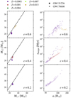 |
Fig. 2. Target regions of the parameter space for GW151226 (square markers) and GW170608 (cross markers) for models with αCE = 1.0. More points are obtained as a result of increasing the grid resolution in the parameter space. |
The solutions obtained for αCE = 2.0 with high metallicities and short initial separations ai < 80 R⊙ merge during the CE phase and thus do not produce BBHs. Additionally, those binaries that end up being compatible progenitors for αCE = 1.0 have smaller separations at BBH formation than their respective αCE = 2.0 runs – and, thus, they all have their associated tmerger effectively reduced.
3.2. Black hole masses
In Fig. 3, we present the distribution of BH masses associated with the progenitors found using αCE = 2.0. Independently of the MT efficiency, the binaries have qBBH ≳ 0.4 and cover the entire range in ℳchirp. Large MT efficiencies (such as ϵ = 0.6) tend to form BBHs with mass ratios closer to unity, while low MT efficiencies (such as ϵ = 0.2) tend to form BBHs with unequal-mass BHs (qBBH ≈ 0.4−0.6). The intermediate scenario (such as ϵ = 0.4) can form BBHs with a broad range of mass ratios, depending on the metallicity.
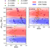 |
Fig. 3. Chirp masses (ℳchirp) and mass ratios (qBBH) of BBHs compatible with GW151226 and/or GW170608 events (within their 100%, 90% and 68% credible intervals in salmon and blue shaded areas, respectively), that merge within the Hubble time for αCE = 2.0. Each panel corresponds to a different value of the MT efficiency. Square (round) markers correspond to binaries with MBH, 2 > MBH, 1 (MBH, 2 < MBH, 1). Different point colours correspond to each metallicity adopted in this work (see legend). |
Those BBHs obtained at lower metallicities span the entire range of mass ratios, while 0.4 ≲ qBBH ≲ 0.7 for the higher metallicities as a consequence of the high mass-loss rates associated with stellar winds. Interestingly, in the latter range of metallicities, for some cases (showed in square markers in Fig. 3), the most massive BH is formed last due to the rejuvenation of the secondary (and initially least massive) star during the stable MT stage. Additionally, at low metallicities, such binaries concentrate along lines of decreasing ℳchirp when qBBH increases.
In Fig. 4, we present BH mass properties obtained with αCE = 1.0. All BBHs have qBBH ≳ 0.5. When ϵ = 0.6, BBHs can also be formed at the highest metallicity. Almost all of them have gone through a rejuvenation process which produced a secondary BH more massive than the primary. On the other hand, in the case when ϵ = 0.4, this is only achieved for the lowest metallicity, whereas in the case of ϵ = 0.2, this is never the case.
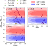 |
Fig. 4. Chirp masses (ℳchirp) and mass ratios (qBBH) of BBHs compatible with GW151226 and/or GW170608 events (within their 100%, 90% and 68% credible intervals in salmon and blue shaded areas, respectively), that merge within the Hubble time for αCE = 1.0. Details as in Fig. 3. |
3.3. Merger time delay
In Figs. 5 and 6, we present the distribution of merger time delay tmerger as a function of ℳchirp for all BBHs with masses compatible to GW151226 or GW170608 for αCE = 2.0 and αCE = 1.0, respectively. When αCE = 2.0 BBHs merge after long delays, we have tmerger ∼ 0.1−10 Gyr, which is comparable to Hubble time, whereas when αCE = 1.0, the mergers occur with shorter delays, that is, tmerger ≲ 1 Gyr, and typically 10–100 Myr.
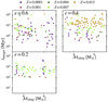 |
Fig. 5. Merger time delay (tmerger) of BBHs compatible with GW151226 or GW170608 (within their 100% C.I.) for αCE = 2.0. Each panel corresponds to different values of the MT efficiency. Different point colours correspond to each metallicity value adopted in this work (see legend). |
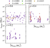 |
Fig. 6. Merger time delay (tmerger) of BBHs compatible with GW151226 or GW170608 (within their 100% C.I.) for αCE = 1.0. Details as in Fig. 5. |
Delay times play a fundamental role in determining the age of the stellar population from which the observed BBHs originate. The results above imply that in the former set of simulations, old binary systems are more involved, while in the latter, younger binary-system progenitors are favoured. However, in this case, high metallicities are strongly disfavoured (except for the highest MT efficiency, ϵ = 0.6), setting strong constraints on the expected properties of their possible host galaxies. Although the contribution of asymmetric natal kicks could change these distributions.
Interestingly, for all simulated binaries, the CE phase is required for the binary to merge within a Hubble time, and merger time delays are strongly impacted by the assumed CE efficiency. As expected, the CE phase plays a fundamental role in BBH mergers in the isolated binary channel. More details can be found in Appendix C.
4. Metallicity-dependent weighted population
The results obtained so far rely over regularly grids that uniformly sample the space of initial masses and separations. In this section, we produce metallicity-dependent population-weighted results, re-scaling via empirical initial mass functions (IMF) for the primary and secondary stars and by an initial separation distribution computed from the observed binary orbital period, 𝒫, distributions.
4.1. Assumptions and methodology
For the mass Mi, 1 of the primary and initially most massive star, we use the IMF from Kroupa et al. (1993):
 (5)
(5)
where α0 = 1.3, α1 = 2.2 and α3 = 2.7, while Mlow = 0.08 M⊙, M0 = 0.5 M⊙, M1 = 1 M⊙, and Mhigh = 150 M⊙.
Given Mi, 1, the mass Mi, 2 of the secondary star is drawn from a flat distribution in the mass ratio q = Mi, 2/Mi, 1,
 (6)
(6)
where qmin = 0.1 and qmax = 1.0.
The initial separation is drawn from the orbital period distribution given in Sana et al. (2012) and de Mink & Belczynski (2015),
 (7)
(7)
where 𝒫 = log Porb in units of days. We note that when drawing the separations from this distribution, we assume zero eccentricity to maintain consistency with our simulations.
Although orbital properties seem to be relatively unaffected by metallicity in the range between the Milky Way and the Large Magellanic Cloud metallicities (Almeida et al. 2017), throughout this work we assume that these distributions are preserved for the entire range of metallicities.
For each metallicity, Z, and MT efficiency, ϵ, we randomly draw 107 binaries from the distributions described above. To get a reasonable resolution, we restrict the random draws to the relevant ranges of masses and separations and keep track of the normalisation constant to account for the rest of the distributions, which is otherwise ignored in the Monte Carlo simulation.
A massive star binary corresponds to a point in the parameter space defined by Mi, 1, Mi, 2 and ai. This point is mapped to the closest point in the regular grid introduced in Sect. 2.5. We assign the properties of the closest binary evolved through the MESA simulations (presented in Sect. 2) to the randomly generated binary This method allows us to obtain statistics that are representative of the entire binary star population, based on numerical simulations of binary stellar evolution. Such a treatment is usually not considered in standard population synthesis simulations as it is computationally expensive.
4.2. Population-weighted results for GW151226 and GW170608
4.2.1. Properties of the initial binaries
Figures 7 and 8 present the probability distributions for the parameters of the initial stellar binaries that eventually evolve into BBHs compatible with GW151226 (dashed lines) and GW170608 (solid lines), assuming αCE = 2.0 and αCE = 1.0, respectively. On the left and middle panels we show the initial masses of the progenitor binaries, Mi, 1 and Mi, 2, respectively. The panels on the right display the initial separations ai. From top to bottom, we show the results obtained with different MT efficiencies (ϵ).
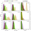 |
Fig. 7. Population-weighted probability distributions for the parameters of the initial star binaries that eventually evolve in BBHs compatible with GW151226 (dashed) and GW170608 (solid) assuming αCE = 2.0. Left and middle panels: component masses Mi, 1 and Mi, 2 of the initial binary and its initial separation ai on the right. From top to bottom, the panels correspond to different MT efficiencies. Colours correspond to the metallicities given in the legend. |
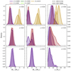 |
Fig. 8. Population-weighted probability distributions for the parameters of the initial star binaries that eventually evolve in BBHs compatible with GW151226 (dashed) and GW170608 (solid) assuming αCE = 1.0. Details as in Fig. 7. |
For αCE = 2.0 (see Fig. 7), progenitors are found in the ∼20–40 M⊙ range for the lower metallicities. For the higher metallicities, the initial masses move into the ∼30–70 M⊙ range, with a stronger dependence on the MT efficiency. In particular, progenitors with solar-like metallicity are not found in the low MT efficiency case (such as ϵ = 0.2, lowest panels). Initial separations cluster at values ≲100 R⊙ but solutions are found up to ∼250 R⊙ for high metallicities. For αCE = 1.0 (Fig. 8), progenitors at solar-like metallicity (Z = 0.015) are only found at the highest MT efficiencies ϵ = 0.6. For the lowest metallicity explored, Z = 0.0001, progenitors are found at every MT efficiency.
The initial masses of the binary progenitors have a clear dependence on metallicity, revealed by two aspects of the distributions: (i) as metallicity increases, more massive progenitors (both primary and secondary masses) are required; (ii) as metallicity increases, the initial-mass distributions widen. This can be interpreted as a consequence of the interplay between wind mass loss and initial binary separation. In initially wide binaries, stellar interactions occur later than in close binaries. Hence, the total mass loss due to stellar winds can operate on different timescales depending on the initial separation. The higher the metallicity, the more pronounced this effect is. Progenitor masses also depend on the MT efficiency assumed. The more inefficient the MT process, the more massive the progenitors are required to be in order to attain the proper target BH masses.
4.2.2. Properties of the binary black holes
Figures 9 and 10 show the parameter distributions of the formed BBHs compatible with GW151226 and GW170608, assuming αCE = 2.0 and αCE = 1.0, respectively.
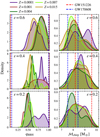 |
Fig. 9. Population-weighted probability distributions for the parameter of the BBHs compatible with GW151226 or GW170608 assuming αCE = 2.0. Left and right panels: mass ratio and chirp mass, respectively. From top to bottom, the panels correspond to different MT efficiencies. Colours correspond to the metallicities given in the legend. The vertical dashed lines indicate the 100% C.I. of qBBH and Mchirp of GW151226 (red) and GW170608 (blue). |
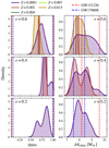 |
Fig. 10. Population-weighted probability distributions for the parameter of the BBHs compatible with GW151226 or GW170608 assuming αCE = 1.0. Details as in Fig. 9. |
When αCE = 2.0 and ϵ ≥ 0.4, the smaller the metallicity the larger the mass of the secondary BH. When Z decreases, the mass-ratio (qBBH = MBBH, 2/MBBH, 1) distribution peak shifts towards unity, and even exceeds 1 for Z ≤ 0.004 and ϵ = 0.6. For low MT efficiency (ϵ = 0.2), secondary BHs are less massive, leading to qBBH < 1. For metallicities Z ≥ 0.001, qBBH ≈ 0.5.
The chirp mass ℳchirp distribution basically spans the entire 100% C.I. for both GW events, independently of the MT efficiency and metallicity. For the largest MT efficiency, ϵ = 0.6, we note a slight preference to form less massive BBHs such as GW170608 instead of GW151226.
When αCE = 1.0, the secondary BH is clearly the heaviest (qBBH > 1) when the MT efficiency is large, ϵ = 0.6. The chirp mass ℳchirp tends to decrease for the solar-like metallicity case. Several narrow distributions obtained are not fully reliable due to the very low statistics available in this case and, thus, they only serve as a guide.
4.2.3. Merger time delay
Figure 11 presents the distribution of the merger time delay tmerger. When αCE = 2.0 (left panels), tmerger clearly increases with metallicity. The distribution peak goes from ∼100 Myr to ∼8 Gyr when Z spans the selected metallicity range, from 0.0001 to 0.015. This correlation disappears for inefficient MT (ϵ = 0.2) and, in this case, lower tmerger values are obtained in general. When αCE = 1.0, since final BBHs are much more compact, merger time delays tend to be reduced by a factor ∼10 with respect to the higher CE efficiency. The merger time delays are thus strongly impacted by the metallicity and the CE phase efficiency.
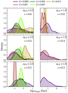 |
Fig. 11. Population-weighted probability distribution of merger time delay (tmerger) of BBHs compatible with GW151226 or GW170608 (within their 100% C.I.). Left (right) panels: αCE = 2.0 (αCE = 1.0). Top to bottom panels: present different values of the MT efficiency adopted throughout this work. Different colours correspond to each metallicity value (see legend). |
As shown in Fig. 11, the merger time delays depend both on the CE efficiency and metallicity. The dependence on metallicity can be understood in terms of the angular momentum carried away by the stellar winds. As lower-metallicity binary progenitors lose less mass, their orbits do not experience significant widening. This leads to final smaller separations for lower-metallicity progenitors, compared to higher metallicity ones.
We notice that it is difficult to make a thorough comparison of the merger delay time distributions with those found in population synthesis studies (Dominik et al. 2012; Giacobbo & Mapelli 2018) given the low stock of available statistics inherent to our study, which is focussed on a narrow range of ℳchirp and does not include natal kicks.
5. Merger rate and gravitational-wave events
We use the population-weighted samples presented in the previous section to estimate the local merger density rate leading to GW events comparable to those studied in this work.
5.1. Method
For binary distributions given by dN = fj(Mi, 1, Mi, 2, ai) dxj, our weighted simulations provide the number density of binaries in the multidimensional space defined by the initial masses, separations, and delay times (tm = T + tmerger ≈ tmerger, where T ≲ 10 Myr is the binary lifetime) that produce each specific GW event, defined as:
 (8)
(8)
where PGW-event is a Kronecker-delta function that selects binaries that evolve into BBHs that are compatible with the considered GW events.
By assuming a cosmology that relates the redshift z to the cosmic time t, the intrinsic GW event rate ℛ(Z,z(t)) can be obtained by integration over the full parameter space:
![Mathematical equation: $$ \begin{aligned} \mathcal{R} \left(Z,z(t)\right)&= \mathcal N_\mathrm {corr}\mathcal \int _0^{t(z)} \int _{M_{\rm i,1}} \int _{M_{\rm i,2}} \int _{a_{\rm i}} \int _0^{t(z)} \dfrac{\mathrm{d}N}{\mathrm{d}M_{\rm i,1} \, \mathrm{d}M_{\rm i,2} \, \mathrm{d}a_{\rm i} \, \mathrm{d}t_{\rm m}}\nonumber \\&\quad \widehat{\mathrm{SFR}} (t^{\prime };Z) \delta \left[ t(z) - (t_{\rm m} + t^\prime ) \right] \mathrm{d}t_{\rm m} \mathrm{d}a_{\rm i} \, \mathrm{d}M_{\rm i,2} \, \mathrm{d}M_{\rm i,1} \, \mathrm{d}t^\prime , \end{aligned} $$](/articles/aa/full_html/2021/05/aa38357-20/aa38357-20-eq14.gif) (9)
(9)
where 𝒩corr is a normalisation factor that includes the total mass ℳT of the 107 simulated binaries, and takes into account the initial masses (𝒩IMF), mass ratios (𝒩q), and separations (𝒩a) excluded from the Monte-Carlo simulation:
 (10)
(10)
where we assume a binary fraction fb = 0.5.
Here,  is the metallicity-dependent star formation rate, namely
 (11)
(11)
where SFR(t′) is the total star formation rate (SFR) history at binary-formation time, t′, in co-moving coordinates (which we adopt from Strolger et al. 2004) and ψ(Z, z′(t′)) accounts for the fraction of stars formed at metallicity, Z.
We divide the full metallicity range into five intervals, namely: ΔZ = 0–0.0005, 0.0005–0.0025, 0.0025–0.005, 0.005–0.0075, and 0.0075–0.03, which we assign to the five simulated values (Z = 0.0001, 0.001, 0.004, 0.007, and 0.015; see Sect. 2). We then compute Ψ(ΔZ, z′) = ∫ΔZψ(Z, z′) dZ, where ψ is normalised to unity, such that  at redshift z′ (Langer & Norman 2006).
Thanks to the δ function in Eq. (9), the summation runs over binary systems at redshift z(t) with appropriate formation time, t′, and merging delay times, tm, and that evolve into BBH merging at cosmic time, t(z). In practice, this integral is evaluated by counting the fraction of sampled binaries per total simulated mass, ℳT, that lead to a BBH merger at the expected redshift or cosmic time. The formation time and delay times are binned with a resolution of 100 Myr.
5.2. Application
Figure 12 shows the dependency of the merger rate density ℛ with the metallicity of the progenitor population and Table 2 compares the local merger rate densities, ℛ(z = 0), that are relevant for predicting GW event rates.
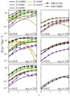 |
Fig. 12. Merger rate density history of events compatible with GW151226 (cross markers) and GW170608 (square markers) as a function of redshift for each metallicity value adopted in this work (see legend for colours). Left panel (right panel): simulations performed using αCE = 2.0 (αCE = 1.0). From the top to bottom panels, we show the results for different MT efficiencies studied in this work. |
Merger rate density at zero redshift for each GW event and αCE. Units are in yr−1 Gpc−3.
The expected local merger rate densities are larger for αCE = 2.0 in every case. This is consistent with the volume of the target regions in the parameter space of compatible binary progenitors, shown in Figs. 1 and 2. As a direct consequence of the chemical evolution, the merger rates decay rapidly at high redshift for the largest metallicities (Z = 0.015 and 0.007), independently of the MT (ϵ) and CE (αCE) efficiencies. Moreover, at the present age (z ≈ 0), the local merger rates decay as a natural consequence of the decay in the SFR.
When αCE = 2.0, in the Local Universe, the rates are correlated with metallicity: the larger the metallicity, the larger the local merger rate density. This is more evident when ϵ = 0.4, and less clear for ϵ = 0.6, where the contributions from all metallicities are more comparable between each other. A slight exception is found for ϵ = 0.2, where no progenitors are found at the maximum (solar-like) metallicity explored. Moreover, in this latter case, the rates are significantly lower than in the former ones.
In the case of αCE = 1.0, the rates decrease by an order of magnitude. The local merger rate density, ℛ(z = 0), is largely dominated by the lowest metallicities, except for ϵ = 0.6, where the high-metallicity progenitors dominate the rates.
5.3. Implications for O1 and O2 science runs
We apply the relation from Dominik et al. (2015) to rescale the intrinsic merger rate from Eq. (9) into GW detection rates:
 (12)
(12)
where w is a geometrical factor, ℳc is the chirp mass of the BBH, Dh is the horizon distance and ℛ is the merger rate density evaluated at z = 0.
Consistently with the highest range for BNS obtained by advanced LIGO and advanced Virgo during their previous science run O2, we consider a binary neutron star (BNS) range Dh = 100 Mpc averaged over all sky directions. The results are shown in Fig. 13 and Table 3. The highest rates are obtained for the highest MT efficiencies (ϵ = 0.4 and 0.6) in both CE cases. For the lowest MT efficiency, the outcome rates are significantly smaller: a factor of 4–5 in the high CE efficiency case, and a factor of ∼10 for the low CE efficiency. Thus, in general, the highest MT efficiency cases are favoured.
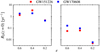 |
Fig. 13. Total detection rates (RD(z = 0)) for O1+O2 LVC observing runs, marginalised over metallicity, as a function of MT efficiency ϵ for αCE = 2.0 (left panel) and αCE = 1.0 (right panel) of events compatible with GW151226 (red) and GW170608 (blue) within their 100% credible intervals. |
Detection rates for O1+O2 LVC observing runs calculated using relation from Dominik et al. (2015) for each GW event and αCE, and considering Dh = 100 Mpc.
In Appendix D, we explore the dependence of the event rates on the assumed star formation history. We find that the strongest differences in event rates are introduced by the metallicity distribution. On the contrary, different SFR histories produce similar outcome rates. These results are compatible with those from Chruslinska & Nelemans (2019), Neijssel et al. (2019) and Tang et al. (2020).
6. Discussion
In this work we study the progenitor properties for the two least-massive BBH mergers (GW151226 and GW170608) detected during the first two science runs of Advanced LIGO and Advanced Virgo, assuming they formed through the so-called isolated binary evolution channel. We simulated a large set of non-rotating stellar models using the binary stellar evolution code MESA (see Appendix A). We investigated a wide range of initial stellar masses, separations, and metallicities. Moreover, to analyse the impact of unconstrained phases of binary evolution related to stellar interactions, we examined the dependence of the outcome results on different efficiencies for stable MT and CE ejection.
In the high CE efficiency scenario (αCE = 2.0), we found progenitors leading to BBH compatible with both GW events, for MT efficiencies ϵ ≥ 0.2. Their initial masses lie in the 20–65 M⊙ mass range for the primary (more massive) star and in the 18–48 M⊙ range for the secondary star. The initial separations are bound to the region 36–200 R⊙. The initial mass ranges depend strongly on the stellar metallicity. This is a direct consequence of the stellar wind efficiencies, as has been pointed out by other authors (e.g., Giacobbo & Mapelli 2018; Kruckow et al. 2018).
The results obtained in the high CE efficiency regime are consistent with other studies in the literature based on different approaches. At low metallicity, Z = 0.001, our results are consistent with Fig. 1 from Stevenson et al. (2017). Furthermore, we obtain similar ranges for the progenitor masses for Z = 0.004−0.007 as Kruckow et al. (2018). Although our highest metallicity differs, our progenitors for GW151226 consistently fall in rather lower mass ranges (Mi, 1 ∼ 45−65 M⊙ instead of ∼80 M⊙, and 35 ≲ Mi, 2 ≲ 48 M⊙ instead of 55 ≲ Mi, 2 ≲ 60 M⊙) given the different BH formation scenario (it is worth mentioning that different MT and CE efficiencies were used).
In the low CE efficiency regime (αCE = 1.0), we obtain a narrower range of initial masses, favouring cases where initial masses are close to equal (q ∼ 1), while initial separations tend to be shifted to higher values, see Fig. 2. In this case a clear relation between the progenitor masses and the metallicity of the population is also recovered. We obtain solutions for the lowest metallicities explored (Z = 0.0001 and 0.001), which exhibit a broad span with regard to the initial separations thanks to the highly-suppressed mass-loss due to stellar winds, which lead to very stable target regions for the binary progenitors.
We find that all these binary systems undergo a CE phase when the primary star has already collapsed to a BH, as expected in the standard BBH formation scenario (Belczynski et al. 2002, 2016; Voss & Tauris 2003; Tauris & van den Heuvel 2006; Dominik et al. 2012), with the companion star either crossing the Hertzsprung gap (HG) or already burning He in its core (CHeB). Although CE phases triggered while the donor star is in the HG when the star does not have a well-defined core-envelope structure (Ivanova & Taam 2004) are usually assumed to lead to a CE merger (Dominik et al. 2012; Spera et al. 2019), by means of our MT treatment (still 1D numerical simulations) we find regions of the explored parameter space populated with binary systems that have survived such a phase. The fraction of binaries in which the donor star is crossing the HG during the CE phase strongly depends on the metallicity due to its impact on the radial expansion of a star (Klencki et al. 2020). We find that this fraction increases from ∼10% for Z = 0.0001 up to ≳90% for Z = 0.015. Moreover, the fraction of such binaries which finish the CE phase without a merger also increases with metallicity from ∼15% to ≳50% from Z = 0.0001 to Z = 0.015, thus having a non-negligible contribution to the population of BBHs, especially at high metallicity. Our simulations show that these low-mass BBHs can only merge in timescales smaller than the Hubble time if they experience a CE phase enabling the ultra-compact binary formation (see also Appendix C).
Additionally, assuming appropriate distributions for the initial-mass function, as well as the binary mass ratios and separations, we calculated the merger rates associated to each GW event for the explored metallicities, which could arise from different formation environments. In the case of αCE = 2.0, we find a correlation between the local merger rate and the metallicity: in general, the higher the metallicity, the higher the rate. This is more evident for ϵ = 0.4. For the lowest MT efficiency, no progenitors are found at solar-like metallicity, which leads to a suppressed final rate. In this case, intermediate metallicities are dominant. On the other hand, for αCE = 1.0, the progenitors tend to be found at the lowest metallicities. We find that a decrease in the CE ejection efficiency produces lower rates in every case. The merger rate density history traces the SFR and, thus, the local merger rates peak at high redshift (z ≳ 1−2). Moreover, the metallicity history has a strong impact on the local merger rates due to younger, solar-like metallicity progenitors with relatively short merger delay times.
In de Mink & Belczynski (2015), the authors show the impact of considering initial binary distributions taken from Sana et al. (2012), as those adopted in this paper, when compared to those from Dominik et al. (2012), which come from Abt (1983). According to their Figs. 1 and 2, the outcome progenitors of the full BBH population found using the former shows shorter periods than those found using the latter distribution. These progenitors mainly accommodate the range between 100 and 1000 days, similarly to the progenitors that we find for the particular low-mass BBH population.
Care must be taken when comparing our derived rates with other works because our focus is set on the detection rate of two particular GW events. For the full BBH population, the LVC reported an empirical rate of ℛ ≃ 9.7−101 yr−1 Gpc−3 (Abbott et al. 2019a), assuming a fixed population distribution, and a BBH merger rate density of  yr−1 Gpc−3 (Abbott et al. 2019b) using different models of the BBH mass and spin distributions, which are naturally higher than the values reported in this work. Our derived detection rates at instrumental sensitivity of Advanced LIGO-Virgo detectors are ∼0.5–3 events per year for αCE = 2.0, and ∼0.01−0.1 for αCE = 1.0, with the former fully consistent with the actual GW events (∼2.1 yr−1 for each event, considering one detection for a total of 167 d of coincident data for O1 and O2 runs, see Abbott et al. 2016b, 2019a). In our simulations with αCE = 2.0 and for the highest MT efficiencies, we obtain rates which are consistent with those found by Kruckow et al. (2018). However, in such cases we also find a comparable rates at intermediate metallicities.
For our high-efficient CE ejection scenario, the lowest metallicities are disfavoured as progenitors of the observed low-mass GW events in the local Universe. In turn, in our simulations, the low-efficient CE scenario is highly disfavoured. In these cases, only low-metallicity progenitors are expected (except for the highest MT efficiency case) with very low merger delay times, which, combined with the metallicity history of the Universe, lead to local merger rates reduced by at least one order of magnitude. Following this trend, we expect even smaller rates for lower CE efficiencies. Although we cannot discard a non-negligible rate for αCE < 1.0, we focussed on the region of the parameter space producing the largest expected rates and compatible with the observed ones. Nevertheless, several recent population synthesis works focusing on the BBH population point to a high CE efficiencies (αCE > 1) when the full BBH population is modelled (Giacobbo & Mapelli 2018; Santoliquido et al. 2020; Wong et al. 2021).
Finally, we caution that all these rates are subject to several uncertainties: when using different values in the input physical parameters, rates can vary by an order of magnitude. For example, it might be unlikely that the efficiency during MT phases remains the same throughout the entire evolution, as rotation might limit accretion from the companion (Packet 1981; Paczynski 1991; Popham & Narayan 1991). Moreover, uncertainties in the mass-loss rates during the luminous blue variable and Wolf–Rayet phases could have an impact on the rates (Barrett et al. 2018). Furthermore, metallicity evolution and star formation rate history were shown to have a strong impact on the BBH merger rates (see, for instance, Neijssel et al. 2019, and our Appendix D). In addition, including asymmetric kicks would also have an influence on the inferred rates. Since the nature of asymmetric kicks remains unknown, kicks are usually treated in a stochastic way. Including asymmetric kicks in our scheme would require running thousands of additional numerical simulations which fall out of the scope of this paper. Thus, in order to estimate the impact that asymmetric kicks could have on our results, in Appendix E we show the outcome of such simulations for a particular binary, leading in this case to a decrease in the intrinsic rates by a factor of ∼3 only.
7. Summary and conclusions
We performed more than 60 000 simulations of binary evolution with the 1D-hydrodynamic MESA code to study the formation history, progenitor properties, and expected rates of the two lowest-mass BBH mergers detected during the O1 and O2 campaigns of LVC. To compute the whole evolution of the binary, we included: (1) the BH formation, through an instantaneous, spherically symmetric ejection, according to the delayed core-collapse prescription from Fryer et al. (2012); and (2) a numerical approach to simulate the CE phase (with two values of the efficiency parameter αCE = 1.0 and 2.0).
Our modelling contains simplified assumptions and limitations that are worth enumerating in this summary. Firstly, asymmetric kicks during BH formation are not incorporated (but see Appendix E for a discussion on the impact expected from natal kicks). Secondly, BH accretion during CE phase is considered negligible. This effect could lead to slightly higher BH masses and, consequently, less massive progenitors (however, see a discussion in Sects. 2 and 5 about the theoretical uncertainties on this particular subject). Thirdly, αCE < 1 is not explored, based on the inferred rates obtained for αCE = 1.0 and 2.0. Then, initially eccentric binaries are not considered mainly due to computational limitations. Orbits may circularise even before the MT onset or on a short timescale during the first MT episode (Verbunt & Phinney 1995). This limitation will have an impact on the distribution of initial binary separations that lead to the GW events under study. Finally, the effects of rotation and tides on the internal mixing are not taken into account.
We summarise below the main results achieved in this work:
-
General remarks: the stellar progenitors of GW151226 are more massive than those of GW170608 (in agreement with the final masses of the black holes). A higher initial orbital separation, ai, implies longer merger times, tmerger. Higher metallicity, Z, implies more massive progenitors (due to mass lost through stellar winds). No progenitors are found for the fully inefficient mass transfer MT (ϵ = 0); for the low-efficiency MT case (ϵ = 0.2), only low Z ≤ 0.001 binaries can become progenitors, whereas for high MT efficiency (ϵ ≥ 0.4), we obtain either solar-like Z progenitors of different masses, or low-Z progenitors evolving towards similar mass stars (mass ratio q close to unity due to rejuvenation process, where the second formed BH becomes more massive than – or at least as massive as – the first); In the case of low CE efficiency (αCE = 1.0), we obtain progenitors having q close to unity (rejuvenation), having only low Z = 0.001−0.0001, except for the highest MT efficiency, where also solar-like Z progenitors are found.
-
Mass ratio and chirp masses:qBBH is always > 0.4, covering all the Mchirp range. High MT efficiencies (ϵ ≥ 0.4) tend to form BBH at any qBBH, while qBBH ∼ 0.4−0.6 for ϵ = 0.2. Low Z stars span whole range of qBBH, showing decreasing Mchirp as qBBH increases. Rejuvenated stars at the highest MT efficiencies lead to qBBH ∼ 1. For αCE = 1.0, progenitors tend towards equal-mass binaries, with all BBHs having qBBH > 0.6 at all Z, and even qBBH > 1.0 for ϵ = 0.6 (rejuvenation process).
-
Merger time delay: for αCE = 2.0, tmerger increases with metallicity, from 10 Myr to 10 Gyr (no correlation, however, for ϵ = 0.2, for which tmerger ∼ 0.1−2 Gyr), while for αCE = 1.0, tmerger is much shorter (due to the late ejection of CE), from ∼5 Myr to ≲1 Gyr (typically 100 Myr); There exists a dichotomy between an old merger population made of high Z progenitors and a young merger population constituted of low Z progenitors. The merger time delay is strongly impacted by both the metallicity and the assumed CE efficiency, with the CE phase always required for binaries to merge within the Hubble time.
-
Merger rate density: Local merger rate densities ℛ(z = 0) are all larger for αCE = 2.0 than αCE = 1.0. ℛ decays rapidly at high redshift for large metallicity (due to the chemical evolution of the universe), independently of αCE. For αCE = 2.0, ℛ ≳ 1 for ϵ ≥ 0.4; For αCE = 1.0, ℛ is mainly dominated by low Z, independently of MT rate.
As a future work, we plan to extend the range of masses of the binary progenitors studied here in order to explore the low-mass end of BH formation and its transition to neutron stars, which could lead to a mass gap in the compact object masses that may be probed with GW observations of BBHs. In addition, more comprehensive modelling that includes stellar rotation and asymmetric kicks is also within the scope of future projects.
Here m1 and m2 are the masses of the donor and accretor at the onset of RLO, respectively.
We assume that a merger occurs in a binary when the reduction in separation leads to a relative donor overflow  bigger than a limiting value which we set equal to 20. We found that beyond this value the donor radius cannot become smaller than its corresponding Roche lobe. Additionally, we assume a merger occurs when the simulations would not complete due to convergence issues at late times during the CE phase.
We refer the reader to Ivanova et al. (2013) for a complete discussion on values of CE efficiency parameter αCE ≥ 1.0.
Acknowledgments
We are grateful to the Referee whose insightful comments helped us to improve the quality of this paper. This work was supported by the LabEx UnivEarthS, Interface project I10, “From evolution of binaries to merging of compact objects”. We acknowledge use of Arago Cluster from Astroparticule et Cosmologie (APC) for our calculations. ASB is a CONICET fellow. We are grateful to the MESA developers for building and making available high-quality computational software for astrophysics. Software: MESA: Modules for Experiments in Stellar Astrophysics, ipython/jupyter (Perez & Granger 2007), matplotlib (Hunter 2007), NumPy (van der Walt et al. 2011), scipy (Jones et al. 2001) and Python from python.org. This research made use of astropy, a community-developed core PYTHON package for astronomy (Astropy Collaboration 2013, 2018).
References
- Abbott, B. P., Abbott, R., Abbott, T. D., et al. 2016a, Phys. Rev. Lett., 116, 241103 [Google Scholar]
- Abbott, B. P., Abbott, R., Abbott, T. D., et al. 2016b, ApJ, 832, L21 [CrossRef] [Google Scholar]
- Abbott, B. P., Abbott, R., Abbott, T. D., et al. 2017a, Phys. Rev. Lett., 119, 161101 [Google Scholar]
- Abbott, B. P., Abbott, R., Abbott, T. D., et al. 2017b, ApJ, 851, L35 [NASA ADS] [CrossRef] [Google Scholar]
- Abbott, B. P., Abbott, R., Abbott, T. D., et al. 2019a, Phys. Rev. X, 9, 031040 [Google Scholar]
- Abbott, B. P., Abbott, R., Abbott, T. D., et al. 2019b, ApJ, 882, L24 [NASA ADS] [CrossRef] [Google Scholar]
- Abt, H. A. 1983, ARA&A, 21, 343 [Google Scholar]
- Acernese, F., Agathos, M., Agatsuma, K., et al. 2015, Class. Quant. Grav., 32, 024001 [Google Scholar]
- Almeida, L. A., Sana, H., Taylor, W., et al. 2017, A&A, 598, A84 [NASA ADS] [CrossRef] [EDP Sciences] [Google Scholar]
- Astropy Collaboration (Robitaille, T. P., et al.) 2013, A&A, 558, A33 [NASA ADS] [CrossRef] [EDP Sciences] [Google Scholar]
- Astropy Collaboration (Price-Whelan, A. M., et al.) 2018, AJ, 156, 123 [Google Scholar]
- Bae, Y.-B., Kim, C., & Lee, H. M. 2014, MNRAS, 440, 2714 [NASA ADS] [CrossRef] [Google Scholar]
- Barrett, J. W., Gaebel, S. M., Neijssel, C. J., et al. 2018, MNRAS, 477, 4685 [NASA ADS] [CrossRef] [Google Scholar]
- Belczynski, K., Kalogera, V., & Bulik, T. 2002, ApJ, 572, 407 [NASA ADS] [CrossRef] [Google Scholar]
- Belczynski, K., Kalogera, V., Rasio, F. A., et al. 2008, ApJS, 174, 223 [NASA ADS] [CrossRef] [Google Scholar]
- Belczynski, K., Holz, D. E., Bulik, T., & O’Shaughnessy, R. 2016, Nature, 534, 512 [Google Scholar]
- Belczynski, K., Klencki, J., Fields, C. E., et al. 2020, A&A, 636, A104 [CrossRef] [EDP Sciences] [Google Scholar]
- Bethe, H. A., & Brown, G. E. 1998, ApJ, 506, 780 [NASA ADS] [CrossRef] [Google Scholar]
- Bhattacharya, D., & van den Heuvel, E. P. J. 1991, Phys. Rep., 203, 1 [NASA ADS] [CrossRef] [Google Scholar]
- Böhm-Vitense, E. 1958, Z. Astrophys., 46, 108 [Google Scholar]
- Brandt, W. N., Podsiadlowski, P., & Sigurdsson, S. 1995, MNRAS, 277, L35 [NASA ADS] [Google Scholar]
- Braun, H., & Langer, N. 1995, A&A, 297, 483 [NASA ADS] [Google Scholar]
- Brott, I., Evans, C. J., Hunter, I., et al. 2011, A&A, 530, A116 [NASA ADS] [CrossRef] [EDP Sciences] [Google Scholar]
- Chruslinska, M., & Nelemans, G. 2019, MNRAS, 488, 5300 [NASA ADS] [Google Scholar]
- De, S., MacLeod, M., Everson, R. W., et al. 2020, ApJ, 897, 130 [CrossRef] [Google Scholar]
- de Jager, C., Nieuwenhuijzen, H., & van der Hucht, K. A. 1988, A&AS, 72, 259 [NASA ADS] [Google Scholar]
- de Kool, M. 1990, ApJ, 358, 189 [NASA ADS] [CrossRef] [Google Scholar]
- de Mink, S. E., & Belczynski, K. 2015, ApJ, 814, 58 [NASA ADS] [CrossRef] [Google Scholar]
- Di Carlo, U. N., Giacobbo, N., Mapelli, M., et al. 2019, MNRAS, 487, 2947 [NASA ADS] [CrossRef] [Google Scholar]
- Dominik, M., Belczynski, K., Fryer, C., et al. 2012, ApJ, 759, 52 [NASA ADS] [CrossRef] [Google Scholar]
- Dominik, M., Berti, E., O’Shaughnessy, R., et al. 2015, ApJ, 806, 263 [NASA ADS] [CrossRef] [Google Scholar]
- Dray, L. M., & Tout, C. A. 2007, MNRAS, 376, 61 [NASA ADS] [CrossRef] [Google Scholar]
- Eldridge, J. J., & Stanway, E. R. 2016, MNRAS, 462, 3302 [NASA ADS] [CrossRef] [Google Scholar]
- Finn, L. S. 1996, Phys. Rev. D, 53, 2878 [NASA ADS] [CrossRef] [Google Scholar]
- Fryer, C. L., & Kalogera, V. 2001, ApJ, 554, 548 [NASA ADS] [CrossRef] [Google Scholar]
- Fryer, C. L., Belczynski, K., Wiktorowicz, G., et al. 2012, ApJ, 749, 91 [NASA ADS] [CrossRef] [Google Scholar]
- Giacobbo, N., & Mapelli, M. 2018, MNRAS, 480, 2011 [NASA ADS] [CrossRef] [Google Scholar]
- Heger, A., Langer, N., & Woosley, S. E. 2000, ApJ, 528, 368 [NASA ADS] [CrossRef] [Google Scholar]
- Hobbs, G., Lorimer, D. R., Lyne, A. G., & Kramer, M. 2005, MNRAS, 360, 974 [NASA ADS] [CrossRef] [Google Scholar]
- Hunter, J. D. 2007, Comput. Sci. Eng., 9, 90 [NASA ADS] [CrossRef] [Google Scholar]
- Iglesias, C. A., & Rogers, F. J. 1993, ApJ, 412, 752 [NASA ADS] [CrossRef] [Google Scholar]
- Iglesias, C. A., & Rogers, F. J. 1996, ApJ, 464, 943 [NASA ADS] [CrossRef] [Google Scholar]
- Ivanova, N., & Taam, R. E. 2004, ApJ, 601, 1058 [NASA ADS] [CrossRef] [Google Scholar]
- Ivanova, N., Justham, S., Chen, X., et al. 2013, A&AR, 21, 59 [Google Scholar]
- Ivanova, N., Justham, S., & Podsiadlowski, P. 2015, MNRAS, 447, 2181 [NASA ADS] [CrossRef] [Google Scholar]
- Janka, H.-T. 2012, Ann. Rev. Nucl. Part. Sci., 62, 407 [Google Scholar]
- Janka, H.-T. 2013, MNRAS, 434, 1355 [Google Scholar]
- Jones, E., Oliphant, T., Peterson, P., et al. 2001, SciPy: Open Source Scientific Tools for Python [Google Scholar]
- Kalogera, V. 1996, ApJ, 471, 352 [NASA ADS] [CrossRef] [Google Scholar]
- Kippenhahn, R., Ruschenplatt, G., & Thomas, H. C. 1980, A&A, 91, 175 [Google Scholar]
- Klencki, J., Nelemans, G., Istrate, A. G., & Pols, O. 2020, A&A, 638, A55 [NASA ADS] [CrossRef] [EDP Sciences] [Google Scholar]
- Kroupa, P., Tout, C. A., & Gilmore, G. 1993, MNRAS, 262, 545 [Google Scholar]
- Kruckow, M. U., Tauris, T. M., Langer, N., et al. 2016, A&A, 596, A58 [NASA ADS] [CrossRef] [EDP Sciences] [Google Scholar]
- Kruckow, M. U., Tauris, T. M., Langer, N., Kramer, M., & Izzard, R. G. 2018, MNRAS, 481, 1908 [Google Scholar]
- Kudritzki, R.-P., & Puls, J. 2000, ARA&A, 38, 613 [NASA ADS] [CrossRef] [Google Scholar]
- Kumamoto, J., Fujii, M. S., & Tanikawa, A. 2020, MNRAS, 495, 4268 [Google Scholar]
- Langer, N., & Norman, C. A. 2006, ApJ, 638, L63 [NASA ADS] [CrossRef] [Google Scholar]
- Langer, N., Fricke, K. J., & Sugimoto, D. 1983, A&A, 126, 207 [NASA ADS] [Google Scholar]
- LIGO Scientific Collaboration (Aasi, J., et al.) 2015, Class.Quant. Grav., 32, 074001 [Google Scholar]
- Lipunov, V. M., Postnov, K. A., & Prokhorov, M. E. 1997, Astron. Lett., 23, 492 [NASA ADS] [Google Scholar]
- MacLeod, M., Antoni, A., Murguia-Berthier, A., Macias, P., & Ramirez-Ruiz, E. 2017, ApJ, 838, 56 [NASA ADS] [CrossRef] [Google Scholar]
- MacLeod, M., & Ramirez-Ruiz, E. 2015, ApJ, 803, 41 [NASA ADS] [CrossRef] [Google Scholar]
- Madau, P., & Fragos, T. 2017, ApJ, 840, 39 [NASA ADS] [CrossRef] [Google Scholar]
- Mandel, I. 2016, MNRAS, 456, 578 [NASA ADS] [CrossRef] [Google Scholar]
- Mandel, I., & de Mink, S. E. 2016, MNRAS, 458, 2634 [NASA ADS] [CrossRef] [Google Scholar]
- Marchant, P., Langer, N., Podsiadlowski, P., Tauris, T. M., & Moriya, T. J. 2016, A&A, 588, A50 [NASA ADS] [CrossRef] [EDP Sciences] [Google Scholar]
- Marchant, P., Langer, N., Podsiadlowski, P., et al. 2017, A&A, 604, A55 [NASA ADS] [CrossRef] [EDP Sciences] [Google Scholar]
- Mirabel, I. F., & Rodrigues, I. 2003, Science, 300, 1119 [NASA ADS] [CrossRef] [PubMed] [Google Scholar]
- Nandez, J. L. A., Ivanova, N., & Lombardi, J. C. J. 2015, MNRAS, 450, L39 [NASA ADS] [CrossRef] [Google Scholar]
- Neijssel, C. J., Vigna-Gómez, A., Stevenson, S., et al. 2019, MNRAS, 490, 3740 [NASA ADS] [CrossRef] [Google Scholar]
- Nugis, T., & Lamers, H. J. G. L. M. 2000, A&A, 360, 227 [NASA ADS] [Google Scholar]
- Packet, W. 1981, A&A, 102, 17 [NASA ADS] [Google Scholar]
- Paczynski, B. 1991, ApJ, 370, 597 [NASA ADS] [CrossRef] [Google Scholar]
- Pavlovskii, K., & Ivanova, N. 2015, MNRAS, 449, 4415 [NASA ADS] [CrossRef] [Google Scholar]
- Pavlovskii, K., Ivanova, N., Belczynski, K., & Van, K. X. 2017, MNRAS, 465, 2092 [NASA ADS] [CrossRef] [Google Scholar]
- Paxton, B., Bildsten, L., Dotter, A., et al. 2010, ApJS, 192, 35 [Google Scholar]
- Paxton, B., Bildsten, L., Dotter, A., et al. 2011, ApJS, 192, 3 [Google Scholar]
- Paxton, B., Cantiello, M., Arras, P., et al. 2013, ApJS, 208, 4 [NASA ADS] [CrossRef] [Google Scholar]
- Paxton, B., Schwab, J., Bauer, E. B., et al. 2018, ApJS, 234, 34 [Google Scholar]
- Paxton, B., Smolec, R., Schwab, J., et al. 2019, ApJS, 243, 10 [Google Scholar]
- Perez, F., & Granger, B. E. 2007, Comput. Sci. Eng., 9, 21 [Google Scholar]
- Peters, P. C. 1964, Phys. Rev., 136, 1224 [Google Scholar]
- Podsiadlowski, P. in Evolution of Binary and Multiple Star Systems, eds. P. Podsiadlowski, S. Rappaport, A. R. King, F. D’Antona, & L. Burderi, ASP Conf. Ser., 229, 239 [Google Scholar]
- Popham, R., & Narayan, R. 1991, ApJ, 370, 604 [NASA ADS] [CrossRef] [Google Scholar]
- Portegies Zwart, S. F., & McMillan, S. L. W. 2000, ApJ, 528, L17 [NASA ADS] [CrossRef] [Google Scholar]
- Quast, M., Langer, N., & Tauris, T. M. 2019, A&A, 628, A19 [NASA ADS] [CrossRef] [EDP Sciences] [Google Scholar]
- Repetto, S., Davies, M. B., & Sigurdsson, S. 2012, MNRAS, 425, 2799 [NASA ADS] [CrossRef] [Google Scholar]
- Ritter, H. 1988, A&A, 202, 93 [NASA ADS] [Google Scholar]
- Rodriguez, C. L., Chatterjee, S., & Rasio, F. A. 2016, Phys. Rev. D, 93, 084029 [NASA ADS] [CrossRef] [Google Scholar]
- Sana, H., de Mink, S. E., de Koter, A., et al. 2012, Science, 337, 444 [Google Scholar]
- Santoliquido, F., Mapelli, M., Bouffanais, Y., et al. 2020, ApJ, 898, 152 [Google Scholar]
- Soberman, G. E., Phinney, E. S., & van den Heuvel, E. P. J. 1997, A&A, 327, 620 [NASA ADS] [Google Scholar]
- Spera, M., Mapelli, M., Giacobbo, N., et al. 2019, MNRAS, 485, 889 [NASA ADS] [CrossRef] [Google Scholar]
- Stevenson, S., Vigna-Gómez, A., Mandel, I., et al. 2017, Nat. Commun., 8, 14906 [NASA ADS] [CrossRef] [Google Scholar]
- Strolger, L.-G., Riess, A. G., Dahlen, T., et al. 2004, ApJ, 613, 200 [NASA ADS] [CrossRef] [Google Scholar]
- Tang, P. N., Eldridge, J. J., Stanway, E. R., & Bray, J. C. 2020, MNRAS, 493, L6 [Google Scholar]
- Tauris, T. M., & van den Heuvel, E. P. J. 2006, in Formation and Evolution of Compact Stellar X-ray Sources, eds. W. H. G. Lewin, & M. van der Klis, 39, 623 [Google Scholar]
- Tauris, T. M., Kramer, M., Freire, P. C. C., et al. 2017, ApJ, 846, 170 [NASA ADS] [CrossRef] [Google Scholar]
- Thorne, K. S., & Zytkow, A. N. 1977, ApJ, 212, 832 [NASA ADS] [CrossRef] [EDP Sciences] [Google Scholar]
- van der Walt, S., Colbert, S. C., & Varoquaux, G. 2011, Comput. Sci. Eng., 13, 22 [Google Scholar]
- Verbunt, F., & Phinney, E. S. 1995, A&A, 296, 709 [NASA ADS] [Google Scholar]
- Vink, J. S., de Koter, A., & Lamers, H. J. G. L. M. 2001, A&A, 369, 574 [NASA ADS] [CrossRef] [EDP Sciences] [Google Scholar]
- Voss, R., & Tauris, T. M. 2003, MNRAS, 342, 1169 [NASA ADS] [CrossRef] [Google Scholar]
- Webbink, R. F. 1984, ApJ, 277, 355 [Google Scholar]
- Wong, K. W. K., Breivik, K., Kremer, K., & Callister, T. 2021, Phys. Rev. D, 103, 083021 [Google Scholar]
Appendix A: MESA runs: full parameter space exploration
As explained in Sect. 2.5, within the frame of this work, we explore a wide range of the parameter space defined by the binary initial parameters: Mi, 1, Mi, 2, and ai with the main goal of finding the target regions of solutions that correspond to models compatible with binary progenitors of the GW170608 and GW151226 events. This task was performed for four different values of MT efficiencies and metallicities. For this purpose, we started with the exploration of the target regions corresponding to αCE = 2.0, which naturally leads to a higher amount of solutions compatible with the GW events with respect to αCE = 1.0 since the fraction of CE mergers is much lower as the CE is more efficiently removed. For this, we used a grid of even numbers for Mi, 1 and odd numbers for Mi, 2 (ΔM = 2 M⊙) and a logarithmic separation in ai of 0.02 dex. We first started by simulating progenitor masses giving CO cores leading to BHs compatible with the observed BH masses and later expanding the regions until no compatible solutions were found. Once these target regions were fully covered, we switched to the exploration of the αCE = 1.0 case. For this, since we already counted with the initial exploration, we focussed on the binary models that lead to CE triggers, which we re-run using the low CE efficiency. Since these target regions are naturally smaller, we decreased the grid to ΔM = 1 M⊙ and 0.01 dex for ai to have a better coverage. For each CE survival, we also simulated the neighbours in the grid until the target regions were fully covered, in an iterative fashion.
In Figs. A.1 and A.2, we present the full parameter space explored using αCE = 2.0 and 1.0, respectively. Panels from top to bottom correspond to each set of MT efficiencies: ϵ = 0.6, 0.4, and 0.2; we do not show the completely inefficient MT case as no compatible progenitors were found. Panels from left to right correspond to each set of metallicities: 0.0001, 0.001, 0.004, 0.007, and 0.015. Blue (red) circles are used for models compatible with GW170608 (GW151226). The size of the circles is proportional to the initial separation (ai). Orange circles represent models leading to BBHs that merge within the Hubble time but with ℳchirp incompatible with the GW events considered. Grey circles are used for the rest of the models used for this work. In Tables A.1 and A.2, we summarise the main characteristics of all the runs performed, including overall total runs, total runs leading to BBHs, total runs leading to BBHs that merge within the Hubble time, and total runs compatible with GW170608 and GW151226 and the ranges covered in the parameter space defined by Mi, 1, Mi, 2 and ai for each MT efficiency (ϵ) and metallicity (Z).
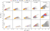 |
Fig. A.1. Full parameter space explored using αCE = 2.0. Blue (red) circles show compatible models with GW170608 (GW151226). Orange circles represent models leading to BBH that merge within the Hubble time, while grey circles are used for the rest of the simulations. |
Summary of MESA runs performed with αCE = 2.0.
Summary of MESA runs performed with αCE = 1.0.
Appendix B: MESA example
In order to illustrate the evolutionary channel explored throughout this work, we present the full evolution of a binary system which ends its evolution as a BBH compatible with one of the events detected by the LVC, using the two values for the CE efficiency (αCE = 2.0 and 1). The initial parameters for the model are: Mi, 1 = 35 M⊙, Mi, 2 = 32 M⊙, ai = 83.05 R⊙, Z = 0.007, and a MT efficiency of ϵ = 0.4.
In Fig. B.1, we present a scheme for the full binary evolution channel followed by the system from ZAMS to the BBH merger. In general, once the primary (most massive) star expands, the system experiences an initial stable MT phase until the primary contracts and later collapses to form a first BH. Later on, once the secondary expands, a new phase of stable MT develops and the system becomes an X-ray binary. If the MT becomes unstable, a short CE phase is triggered, and the binary separation is heavily reduced while the donor envelope is removed. After separation, a second BH is formed leading to a BBH that will eventually coalesce through the emission of GWs.
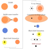 |
Fig. B.1. Schematic view of the binary evolutionary channel explored throughout this work. |
In Fig. B.2, we present the full binary evolution Hertzsprung–Russell (HR) diagram corresponding to the example binary systems. In this HR diagram, the primary and secondary stars are born in the ZAMS (in the bottom right part of the figure) and end by forming BHs (in the upper left part of the plot). After the primary star expands, two stable MT phases develop: the so-called cases AB and B indicated in light-blue and green, respectively. The luminosity of the primary increases until separation occurs. Then, the primary contracts, moving to the left forming a Wolf–Rayet star. Later on, it collapses to a BH (black star in the figure). Meanwhile, the secondary continues its evolution. After leaving the MS, the secondary expands and a stable MT phase commences (Case AB to BH indicated with salmon colour). This continues until an unstable CE phase is triggered (at the grey circle). A fast out-of-equilibrium phase is developed until separation of the secondary occurs at the blue and orange circles, for αCE = 2.0 and 1, respectively. The secondary evolution then continues until a second BH is formed.
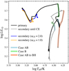 |
Fig. B.2. Full binary evolution HR diagram of the binary system considered in the example. Primary and secondary stars are born in the ZAMS (bottom right). Case AB (B) stable MT phase is indicated in light-blue (green). Afterwards, the primary moves to the left and collapses to form a first BH (black star). The secondary expands and a case AB stable MT phase occurs (salmon colour) until an unstable CE phase is triggered (grey circle). The detach of the secondary occurs at the blue (orange) circle for αCE = 2.0 (αCE = 1.0). A second BH is formed at the top left corner (coloured stars). |
During the short (on the order of ∼100 yr) unstable CE phase, the binary system evolves quickly as the orbital energy is extracted to unbind the envelope of the donor. In Fig. B.3 we show the evolution of the binary parameters during the CE phase for both CE efficiencies. In the top panel, we show the evolution of the donor mass loss (ṀRLOF), in the mid panel the binary separation (a) and in the bottom panel, we show the relative overflow defined as f(R, RRL) = (R − RRL)/RRL. Furthermore, in Fig. B.4, we focus on the evolution of the donor parameters. From top to bottom, we present the donor radius, total mass, superficial H mass fraction, and relative overflow.
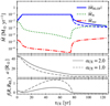 |
Fig. B.3. Evolution of binary parameters across the CE phase. In the top panel, we present the evolution of the donor mass loss (ṀRLOF, blue) and mass transfer scales: thermal (Ṁth, dotted green) and nuclear (Ṁnuc, dot-dashed red). In the mid panel, the separation (a) and in the lower panel the relative overflow (f(R, RRL)). Solid (dashed) lines represent αCE = 2.0 (αCE = 1.0). |
 |
Fig. B.4. Evolution of donor star parameters during the CE phase. From top to bottom, we present the evolution of the donor radius (R), donor total mass (M), superficial H mass fraction, and the relative overflow (f(R, RRL)). Solid (dashed) lines represent αCE = 2.0 (αCE = 1.0). |
Once the CE is triggered (τCE = 0), the donor mass loss grows linearly for 10 yr from stable MT value to the fixed rate of 10−1 M⊙ yr−1. During the early phase, the binary separation shrinks faster than the donor radius and thus the relative overflow increases, until this effect is reversed at 50–60 yr. After that, the donor star shrinks faster until separation is reached at ∼80 yr, after the beginning of the CE phase. At this point, the mass loss rate decreases until the thermal scale is recovered (ṀRLOF ≈ Ṁth) and the CE phase is finished. As a result of the CE phase, the envelope of the donor star is removed. In particular, in the αCE = 1.0 case, no H is left, while in the αCE = 2.0 case a small fraction of H remains, but its total mass decreases by ∼7 M⊙. In both cases, a strong decrease of a factor of ∼10 in the orbital separation is seen, leading to an ultra-compact binary which eventually will become a BBH that will merge within the Hubble time.
Appendix C: Merger time delay calculation
In a binary consisting of two BHs, orbital shrinking is driven by the emission of gravitation waves, which ends up with a merger of the BHs. In order to estimate the time needed for a BBH to merge after its formation, which is also known as merger time delay, we use the prescription given by Peters (1964):
![Mathematical equation: $$ \begin{aligned} t_{\rm merger}&= \dfrac{15}{304} \dfrac{a_{0}^{4} c^{5}}{G^{3} m_{1} m_{2} (m_{1} + m_{2})} \nonumber \\&\quad \times \left[\left(1+e_{0}^{2}\right) e_{0}^{-12/19} \left(1 + \dfrac{121}{304} e_{0}^{2} \right)^{-870/2299}\right]^{4} \nonumber \\&\quad \times \int _{0}^{e_{0}} \mathrm{d}e \dfrac{e^{29/19} \left[1+\left(121/304\right)e^{2}\right]^{1181/2299}}{\left(1-e^{2}\right)^{3/2}}, \end{aligned} $$](/articles/aa/full_html/2021/05/aa38357-20/aa38357-20-eq22.gif) (C.1)
(C.1)
where a0 and e0 are the semi-major axis and eccentricity at BBH formation, while m1 and m2 are the BH masses.
We show in Fig. C.1 all the BBHs found in our simulations that lie inside the 100% C.I. of GW151226 or GW170608. Two different sub-populations can be seen: binaries that went through a CE phase and those which did not. The former have aBBH < 30−40 R⊙ and most of them have a merger time delay lower than the Hubble time, while the latter have aBBH ≳ 30−40 R⊙ and hence, merger time delays longer than the Hubble time. Therefore, the CE phase plays a key role in the formation of ultra-compact binaries which are progenitors of GW151226 and GW170608 in this evolutionary channel. Since we do not consider asymmetric BH kicks and the ejected masses in the BH prescription adopted are small (due to fallback), the BBH eccentricities arising from our simulations are generally constrained to eBBH ≲ 0.25. As can be seen in Fig. C.1, for these eccentricity values, aBBH ≲ 20 R⊙ are needed to produce BBHs with merger time delays below the Hubble time. This is because merger time delays strongly depend on the separation at BBH formation: increasing it by a factor of 10 leads to an increase in tmerger of a factor 104.
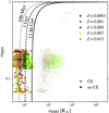 |
Fig. C.1. Final binary parameters for all our BBHs with ℳchirp consistent with GW151226 or GW170608. Colours indicate different metallicities (see legend). Dotted, dashed, and solid black lines correspond to values of constant tmerger: 100 Myr, 1 Gyr, τHubble, respectively, assuming BH masses of 12.3 and 7.65 M⊙. |
Appendix D: Dependence of the merger rates on the star formation history
Neijssel et al. (2019) show that the uncertainties in the metallicity evolution and star formation history can change the rates of BBH mergers. Thus, we perform the evaluation of detectable rates during O1/O2 observing runs for the progenitor population of the GW151226 and GW170608 for different SFRs and metallicity distributions. In addition to the previously mentioned SFR from Strolger et al. (2004), we use the SFR from Madau & Fragos (2017). For the evolution of metallicity over cosmic time, we compare the distribution from Langer & Norman (2006) with that of the fiducial model of Neijssel et al. (2019).
In Fig. D.1 we present merger rates for different combinations of star-formation evolution over cosmic time. Our results show that the strongest changes in event rates are introduced by the metallicity distribution, while the different SFRs assumed produce fewer variations in the outcome rates. These results are similar to the ones found by Chruslinska & Nelemans (2019) and Neijssel et al. (2019). For some cases, we find differences in the rates of more than a factor of two. In all cases, the maximum value for the detection rate remains at a level of a few per year.
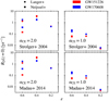 |
Fig. D.1. Total detection rates for O1 and O2 runs, RD(z = 0), marginalised over metallicity, as a function of MT efficiency ϵ for αCE = 2.0 (left panel) and αCE = 1.0 (right panel) of events compatible with GW151226 (red) and GW170608 (blue) within their 100% credible intervals. Circles represent detection rates assuming the metallicity evolution given in Langer & Norman (2006) while rectangles are the rates found using the metallicity distribution of Neijssel et al. (2019). |
Appendix E: Black hole kicks
One important and rather uncertain aspect of massive binary evolution is connected to the momentum imparted during the formation of a BH, that is, the ‘natal kick’, which is similar to those that NSs receive during their formation (Janka 2012). This kick onto a BH could happen if, instead of having a direct collapse, a proto-NS is formed and a weak explosion leads to a large amount of mass falling back, whereas a small envelope becomes unbound (Brandt et al. 1995; Fryer & Kalogera 2001). Although the magnitude of the kick for NSs is rather well constrained from pulsar observations (Hobbs et al. 2005), the strength of natal kicks imparted onto BHs is an open issue given the ongoing debate that features some arguments in favour of weak kicks (Mirabel & Rodrigues 2003; Mandel 2016), while others favour the opposite (Repetto et al. 2012; Janka 2013).
Here, we present the effect introduced by considering natal kicks during the formation of a BH for each of the two core-collapse stages needed to produce a BBH system. Modelling kicks for all the first formed BHs in our sample is a difficult task in this case as it involves drawing different velocities and directions, and then running detailed simulations for each of them. Instead, to quantify the effect of kicks, we choose one of all the simulations performed, which we identified as having consistent masses with one of the GW events under study. After the primary collapses into a BH, we randomly draw 500 kicks from a Maxwellian distribution with a speed of 265 km s−1 reduced by a factor (1 − ffb), where ffb is the fraction of mass that falls back onto the proto-NS (Fryer et al. 2012), isotropically orientated. The post-kick binary parameters (separation and eccentricity) are updated following Kalogera (1996), assuming no interaction between the ejected mass at BH formation and the companion star. Once this initial conditions are set, each binary is evolved with MESA (as described in Sect. 2.2).
In Fig. E.1, we show all possible post-kick binaries which remain bound after the first core-collapse (which represent ∼53% of all simulated binaries). Each point in the figure represents a binary evolved using MESA, consisting of a BH and its companion star. We find that binaries with post-kick separations that are shorter than the one they had previous to the core-collapse tend to go through a CE phase which leads to the merger of the components, while binaries with larger separations, successfully eject the envelope, subsequently detaching and reaching a second core-collapse stage.
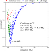 |
Fig. E.1. Binary configurations after applying a natal kick during the formation of the first BH. Masses and separations shown correspond to pre-collapse orbital parameters. Each point represents a single detailed binary evolution of the BH and its companion star. Colours show different binary outcomes: in green, we represent merging binaries during a CE phase, in red we show binaries which unexpectedly end due to numerical problems, while blue points are binaries reaching the second core-collapse stage. The arrow represents the location on this plane of the binary that receives no natal kick. |
For each of the binaries reaching the second BH formation, we randomly apply 500 more kicks from the same distributions mentioned before and compute the fraction of BBHs that end up merging within the Hubble time. The outcoming distribution of binary parameters at BBH formation are shown in Fig. E.2. As described before, the no-kick case is a progenitor candidate to the GW events under study, as it produces a BBH system at the end of its evolution, having a merger time of 0.2 Gyr. For this chosen system, we obtain a ∼30% probability that it would merge in less than a Hubble time if the described asymmetric kicks were applied (the remaining ∼70% of the simulations are either unbound or they have a much longer merger time than the Hubble time); the chances of the system being disrupted during the second core-collapse is less than 2%. Thus, we can expect that the addition of considering natal kicks imparted onto the BHs during both core-collapse stages would decrease the derived intrinsic rates by a factor of ∼3. We note, however, that we cannot discard, as a contribution to the merger rate, the case of BBHs formed from wider stellar binaries experiencing a fine-tuned kick, leading them to an ultra-compact remnant and then allowing them to merge within a Hubble time.
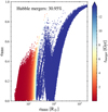 |
Fig. E.2. Binary configurations after the formation of the second BH. Each point corresponds to one of the 500 binaries randomly drawn from the blue points in Fig. E.1. Colours indicate the merger delay times of the post-collapse BBHs as a result of gravitational wave radiation. After this kick, there is a 30% chance that the BHs merge within the Hubble time. |
All Tables
Merger rate density at zero redshift for each GW event and αCE. Units are in yr−1 Gpc−3.
Detection rates for O1+O2 LVC observing runs calculated using relation from Dominik et al. (2015) for each GW event and αCE, and considering Dh = 100 Mpc.
All Figures
|
Fig. 1. Target regions of the parameter space for GW151226 (square markers) and GW170608 (cross markers) for models with αCE = 2.0. Left panels: progenitor initial masses (Mi, 1 > Mi, 2). Right panels: merger time delay (tmerge) against initial binary separation (ai). Panels from top to bottom correspond to each set of efficiencies: ϵ = 0.6, 0.4, 0.2. Dashed lines indicate equal progenitor masses. |
| In the text | |
|
Fig. 2. Target regions of the parameter space for GW151226 (square markers) and GW170608 (cross markers) for models with αCE = 1.0. More points are obtained as a result of increasing the grid resolution in the parameter space. |
| In the text | |
|
Fig. 3. Chirp masses (ℳchirp) and mass ratios (qBBH) of BBHs compatible with GW151226 and/or GW170608 events (within their 100%, 90% and 68% credible intervals in salmon and blue shaded areas, respectively), that merge within the Hubble time for αCE = 2.0. Each panel corresponds to a different value of the MT efficiency. Square (round) markers correspond to binaries with MBH, 2 > MBH, 1 (MBH, 2 < MBH, 1). Different point colours correspond to each metallicity adopted in this work (see legend). |
| In the text | |
|
Fig. 4. Chirp masses (ℳchirp) and mass ratios (qBBH) of BBHs compatible with GW151226 and/or GW170608 events (within their 100%, 90% and 68% credible intervals in salmon and blue shaded areas, respectively), that merge within the Hubble time for αCE = 1.0. Details as in Fig. 3. |
| In the text | |
|
Fig. 5. Merger time delay (tmerger) of BBHs compatible with GW151226 or GW170608 (within their 100% C.I.) for αCE = 2.0. Each panel corresponds to different values of the MT efficiency. Different point colours correspond to each metallicity value adopted in this work (see legend). |
| In the text | |
|
Fig. 6. Merger time delay (tmerger) of BBHs compatible with GW151226 or GW170608 (within their 100% C.I.) for αCE = 1.0. Details as in Fig. 5. |
| In the text | |
|
Fig. 7. Population-weighted probability distributions for the parameters of the initial star binaries that eventually evolve in BBHs compatible with GW151226 (dashed) and GW170608 (solid) assuming αCE = 2.0. Left and middle panels: component masses Mi, 1 and Mi, 2 of the initial binary and its initial separation ai on the right. From top to bottom, the panels correspond to different MT efficiencies. Colours correspond to the metallicities given in the legend. |
| In the text | |
|
Fig. 8. Population-weighted probability distributions for the parameters of the initial star binaries that eventually evolve in BBHs compatible with GW151226 (dashed) and GW170608 (solid) assuming αCE = 1.0. Details as in Fig. 7. |
| In the text | |
|
Fig. 9. Population-weighted probability distributions for the parameter of the BBHs compatible with GW151226 or GW170608 assuming αCE = 2.0. Left and right panels: mass ratio and chirp mass, respectively. From top to bottom, the panels correspond to different MT efficiencies. Colours correspond to the metallicities given in the legend. The vertical dashed lines indicate the 100% C.I. of qBBH and Mchirp of GW151226 (red) and GW170608 (blue). |
| In the text | |
|
Fig. 10. Population-weighted probability distributions for the parameter of the BBHs compatible with GW151226 or GW170608 assuming αCE = 1.0. Details as in Fig. 9. |
| In the text | |
|
Fig. 11. Population-weighted probability distribution of merger time delay (tmerger) of BBHs compatible with GW151226 or GW170608 (within their 100% C.I.). Left (right) panels: αCE = 2.0 (αCE = 1.0). Top to bottom panels: present different values of the MT efficiency adopted throughout this work. Different colours correspond to each metallicity value (see legend). |
| In the text | |
|
Fig. 12. Merger rate density history of events compatible with GW151226 (cross markers) and GW170608 (square markers) as a function of redshift for each metallicity value adopted in this work (see legend for colours). Left panel (right panel): simulations performed using αCE = 2.0 (αCE = 1.0). From the top to bottom panels, we show the results for different MT efficiencies studied in this work. |
| In the text | |
|
Fig. 13. Total detection rates (RD(z = 0)) for O1+O2 LVC observing runs, marginalised over metallicity, as a function of MT efficiency ϵ for αCE = 2.0 (left panel) and αCE = 1.0 (right panel) of events compatible with GW151226 (red) and GW170608 (blue) within their 100% credible intervals. |
| In the text | |
|
Fig. A.1. Full parameter space explored using αCE = 2.0. Blue (red) circles show compatible models with GW170608 (GW151226). Orange circles represent models leading to BBH that merge within the Hubble time, while grey circles are used for the rest of the simulations. |
| In the text | |
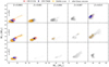 |
Fig. A.2. Full parameter space explored using αCE = 1.0. Details as in Fig. A.1. |
| In the text | |
|
Fig. B.1. Schematic view of the binary evolutionary channel explored throughout this work. |
| In the text | |
|
Fig. B.2. Full binary evolution HR diagram of the binary system considered in the example. Primary and secondary stars are born in the ZAMS (bottom right). Case AB (B) stable MT phase is indicated in light-blue (green). Afterwards, the primary moves to the left and collapses to form a first BH (black star). The secondary expands and a case AB stable MT phase occurs (salmon colour) until an unstable CE phase is triggered (grey circle). The detach of the secondary occurs at the blue (orange) circle for αCE = 2.0 (αCE = 1.0). A second BH is formed at the top left corner (coloured stars). |
| In the text | |
|
Fig. B.3. Evolution of binary parameters across the CE phase. In the top panel, we present the evolution of the donor mass loss (ṀRLOF, blue) and mass transfer scales: thermal (Ṁth, dotted green) and nuclear (Ṁnuc, dot-dashed red). In the mid panel, the separation (a) and in the lower panel the relative overflow (f(R, RRL)). Solid (dashed) lines represent αCE = 2.0 (αCE = 1.0). |
| In the text | |
|
Fig. B.4. Evolution of donor star parameters during the CE phase. From top to bottom, we present the evolution of the donor radius (R), donor total mass (M), superficial H mass fraction, and the relative overflow (f(R, RRL)). Solid (dashed) lines represent αCE = 2.0 (αCE = 1.0). |
| In the text | |
|
Fig. C.1. Final binary parameters for all our BBHs with ℳchirp consistent with GW151226 or GW170608. Colours indicate different metallicities (see legend). Dotted, dashed, and solid black lines correspond to values of constant tmerger: 100 Myr, 1 Gyr, τHubble, respectively, assuming BH masses of 12.3 and 7.65 M⊙. |
| In the text | |
|
Fig. D.1. Total detection rates for O1 and O2 runs, RD(z = 0), marginalised over metallicity, as a function of MT efficiency ϵ for αCE = 2.0 (left panel) and αCE = 1.0 (right panel) of events compatible with GW151226 (red) and GW170608 (blue) within their 100% credible intervals. Circles represent detection rates assuming the metallicity evolution given in Langer & Norman (2006) while rectangles are the rates found using the metallicity distribution of Neijssel et al. (2019). |
| In the text | |
|
Fig. E.1. Binary configurations after applying a natal kick during the formation of the first BH. Masses and separations shown correspond to pre-collapse orbital parameters. Each point represents a single detailed binary evolution of the BH and its companion star. Colours show different binary outcomes: in green, we represent merging binaries during a CE phase, in red we show binaries which unexpectedly end due to numerical problems, while blue points are binaries reaching the second core-collapse stage. The arrow represents the location on this plane of the binary that receives no natal kick. |
| In the text | |
|
Fig. E.2. Binary configurations after the formation of the second BH. Each point corresponds to one of the 500 binaries randomly drawn from the blue points in Fig. E.1. Colours indicate the merger delay times of the post-collapse BBHs as a result of gravitational wave radiation. After this kick, there is a 30% chance that the BHs merge within the Hubble time. |
| In the text | |
Current usage metrics show cumulative count of Article Views (full-text article views including HTML views, PDF and ePub downloads, according to the available data) and Abstracts Views on Vision4Press platform.
Data correspond to usage on the plateform after 2015. The current usage metrics is available 48-96 hours after online publication and is updated daily on week days.
Initial download of the metrics may take a while.