| Issue |
A&A
Volume 647, March 2021
|
|
|---|---|---|
| Article Number | A186 | |
| Number of page(s) | 9 | |
| Section | Interstellar and circumstellar matter | |
| DOI | https://doi.org/10.1051/0004-6361/202039779 | |
| Published online | 01 April 2021 | |
High-accuracy estimation of magnetic field strength in the interstellar medium from dust polarization
1
Institute of Astrophysics, Foundation for Research and Technology-Hellas,
Vasilika Vouton,
70013
Heraklion, Greece
2
Department of Physics & ITCP, University of Crete,
70013
Heraklion,
Greece
e-mail: This email address is being protected from spambots. You need JavaScript enabled to view it.
; This email address is being protected from spambots. You need JavaScript enabled to view it.
Received:
28
October
2020
Accepted:
3
February
2021
Abstract
Context. A large-scale magnetic field permeates our Galaxy and is involved in a variety of astrophysical processes, such as star formation and cosmic ray propagation. Dust polarization has been proven to be one of the most powerful observables for studying the field properties in the interstellar medium (ISM). However, it does not provide a direct measurement of its strength. Different methods have been developed that employ both polarization and spectroscopic data in order to infer the field strength. The most widely applied method was developed by Davis (1951, Phys. Rev., 81, 890) and Chandrasekhar & Fermi (1953, ApJ, 118, 1137), hereafter DCF. The DCF method relies on the assumption that isotropic turbulent motions initiate the propagation of Alfvén waves. Observations, however, indicate that turbulence in the ISM is anisotropic and that non-Alfvénic (compressible) modes may be important.
Aims. Our goal is to develop a new method for estimating the field strength in the ISM that includes the compressible modes and does not contradict the anisotropic properties of turbulence.
Methods. We adopt the following assumptions: (1) gas is perfectly attached to the field lines; (2) field line perturbations propagate in the form of small-amplitude magnetohydrodynamic (MHD) waves; and (3) turbulent kinetic energy is equal to the fluctuating magnetic energy. We use simple energetics arguments that take the compressible modes into account to estimate the strength of the magnetic field.
Results. We derive the following equation: B0 = √2πρδv/√δθ, where ρ is the gas density, δv is the rms velocity as derived from the spread of emission lines, and δθ is the dispersion of polarization angles. We produce synthetic observations from 3D MHD simulations, and we assess the accuracy of our method by comparing the true field strength with the estimates derived from our equation. We find a mean relative deviation of 17%. The accuracy of our method does not depend on the turbulence properties of the simulated model. In contrast, the DCF method, even when combined with the Hildebrand et al. (2009, ApJ, 696, 567) and Houde et al. (2009, ApJ, 706, 1504) method, systematically overestimates the field strength.
Conclusions. Compressible modes can significantly affect the accuracy of methods that are based solely on Alfvénic modes. The formula that we propose includes compressible modes; however, it is applicable only in regions with no self-gravity. Density inhomogeneities may bias our estimates to lower values.
Key words: ISM: magnetic fields / magnetohydrodynamics (MHD) / polarization
© ESO 2021
1 Introduction
The Galactic magnetic field plays a key role in various astrophysical processes, such as cosmic ray propagation and star formation, and affects foregrounds relevant to cosmic microwave background polarization experiments. Various tracers that reveal either the line of sight (LOS) or the plane of the sky (POS) component of the field exist. Zeeman splitting is sensitive to the LOS component and is the only observable that reveals both the LOS local magnitude and the orientation of the field vector along this direction. Regarding the POS component, synchroton and dust polarization are the most common observables. Unlike synchroton, dust polarization traces the POS field in the cold neutral medium, where stars form. Dust polarization reveals only the morphology of the field, not its strength (see Andersson et al. 2015, for a recent review). Different magnetic field strength estimation methods have been developed using the dust polarization data.
The first method was presented by Davis (1951) and Chandrasekhar & Fermi (1953), hereafter DCF. They assumed that magnetic field lines are distorted due to the propagation of the incompressible transverse magnetohydrodynamic (MHD) waves, known as Alfvén waves. This distortion induces a spread in the polarization angle distribution, which, combined with the gas turbulent motions from spectroscopic data, allows the estimate of the true magnetic field strength. Different effects have been recognized to bias the accuracy of the DCF method toward higher values (Zweibel 1990; Myers & Goodman 1991). Ostriker et al. (2001), Padoan et al. (2001), and Heitsch et al. (2001), after testing the accuracy of the method in MHD simulations, found that, on average, the method produces a two-fold deviation. In addition, it was realized that external forces, such as self-gravity, can bend the field lines and induce extra dispersion in the polarization angle distribution. In order to address the problem, Girart et al. (2006) fitted parabolas to the polarization data and removed the large-scale hour-glass bending from the polarization data of a pre-stellar core. A similar, but more sophisticated, approach was followed by Pattle et al. (2017). On the other hand, Hildebrand et al. (2009) and Houde et al. (2009), hereafter HH09, developed an analytical model for the polarization data that measures the turbulence-induced spread in the presence of any external source of B-field bending. Modifications of the DCF method have been developed by Heitsch et al. (2001), Kudoh & Basu (2003), Falceta-Gonçalves et al. (2008), Cho & Yoo (2016), Yoon & Cho (2019), and Lazarian et al. (2020). Recent reviews are available in Pattle & Fissel (2019) and Hull & Zhang (2019). “All these methods rely on the assumption that the Alfvén waves produce the observed polarization angle dispersion and the linewidths in the emission spectra.”
The interstellar medium (ISM) is highly compressible and, in addition to Alfvén waves, contains MHD wave modes that induce density compressions. These are known as fast and slow magnetosonic modes, and their existence in astrophysical plasmas is inevitablebecause they are excited by the Alfvén waves (e.g., Heyvaerts & Priest 1983). In addition, the so-called entropy modes can contribute to the observed compressibility of the ISM (Lithwick & Goldreich 2001); however, they produce zero velocity as well as magnetic field fluctuations. All the aforementioned methods ignore the existence of the compressible modes. This can lead to significant inaccuracies in the magnetic field strength estimates.
In the present work, we propose a new relation for estimating the field strength, which, unlike the DCF method, “includes the compressible modes”. We assess the validity of our method using synthetic observations that we produce from 3D MHD turbulence simulations. Our method employs both polarization and spectroscopic data. Its applicability should be restricted to regions that do not show large-scale bending due to self-gravity.
The structure of the paper is as follows. In Sect. 2, we critically review the DCF method, including its underline assumptions, and point out projection effects that may affect its accuracy. We also test the method in 3D simulations. In Sect. 3, we critically review the HH09 method, and we apply it in synthetic observations of 3D simulations. In Sect. 4, we present our new method, apply it in 3D simulations, and discuss its limitations. In Sect. 5, we summarize our results.
2 Classical DCF method
2.1 Foundations of the method
We decomposed the total magnetic field into a mean component, B0, and a fluctuating component, δB. The total field is B = B0 + δB with a total magnetic energy density equal to
![Mathematical equation: \begin{equation*}\frac{B^{2}}{8\pi}\,{=}\,\frac{1}{8\pi} [B_{0}^{2} + \delta B^{2} + 2 \bm{\delta B} \cdot \bm{B}_{0}], \end{equation*}](/articles/aa/full_html/2021/03/aa39779-20/aa39779-20-eq2.png) (1)
(1)
where bold letters are used to denote vectors. The last two terms correspond to changes in the magnetic energy, δϵm, due to δB fluctuations. The DCF method assumes that the ISM plasma conductivity is infinite. This means that the magnetic field is “frozen” in the gas, and hence both gas and field lines oscillate in phase. Turbulent gas motions perturb the field lines and initiate small amplitude fluctuations, |δB|≪|B0|, around the mean field “in the form of Alfvén waves”. DCF assumed that the kinetic energy of turbulent motions will be equal to the fluctuating magnetic energy density
 (2)
(2)
where ρ is the gas density and δv is the rms velocity. We note that B0 ⋅ δB = 0 since Alfvén waves are transverse. We divided both sides by  , and after rearranging we obtained
![Mathematical equation: \begin{equation*} B_{0}\,{=}\,\sqrt{4 \pi \rho} \delta v \Bigg [ \frac{\delta B}{{B_{0}}} \Bigg ]^{-1}. \end{equation*}](/articles/aa/full_html/2021/03/aa39779-20/aa39779-20-eq5.png) (3)
(3)
The magnetic field orientation is traced by dust polarization (with a π ambiguity), and the dispersion of the polarization angle distribution, δθ, is a metric of δB∕B0. If the mean field is stronger than the fluctuating component, the field lines will appear approximately straight, and hence δθ will be small. If, on the other hand, the fluctuations are relatively large, field lines will be dispersed by turbulent motions and δθ will increase. Thus, DCF assumed δθ = δB∕B0, yielding
 (4)
(4)
where the factor  was inserted by DCF because they assumed that turbulent motions are isotropic and that only one of the three Cartesian velocity components perturbs the field lines. Other authors (see Ostriker et al. 2001) proposed a different correction factor, f. The generalized DCF equation is then
 (5)
(5)
The mean magnetic field, B0, can be written in velocity units by dividing it by  , thus
 (6)
(6)
where VA is the Alfvén speed.
2.2 Caveats of the method
The DCF approach is based on the assumption of an equipartition between kinetic and magnetic energy, which holds for traveling MHD waves. For standing waves, the total energy oscillates between magnetic and kinetic forms. Since our observables (polarization angles and spectroscopic data) are instantaneous, equipartition between kinetic and magnetic energies can only happen in standing waves twice in a phase cycle. Standing waves have been produced in MHD simulations (Kudoh & Basu 2003) and have been identified in the ISM, for example in the Musca molecular cloud (Tritsis & Tassis 2018). In this paper, we consider only traveling MHD waves.
2.2.1 Turbulent velocities and compressible modes
The DCF method has been used extensively in atomic and molecular clouds. Turbulent velocities, denoted as δv or σv, are measured using spectroscopic data (e.g., the HI 21cm line, the CO(J = 1–0) line, etc.). Emission lines are approximated as Gaussians, and nonthermal linewidths are usually observed. The nonthermal broadening, σv,turb, is attributed to turbulent gas motions, and thus
 (7)
(7)
where σv,tot is the total observed spread and σv,thermal is the thermal broadening.
Turbulent broadening, σv,turb, may containcontributions from wave modes other than the Alfvén modes. MHD plasma also supports the propagation of fast and slow modes, which can be excited even if they are not initially in the system (Heyvaerts & Priest 1983) due to their coupling with Alfvén modes. These modes can induce extra dispersion in the observed velocities and significantly affect the DCF method, which neglects their contribution.
The ISM is highly compressible (e.g., Heiles & Troland 2003). This implies that σv,turb includes velocities from both Alfvén and compressible modes. As a result, σv,turb will always be higher than when there are only Alfvén waves, and hence B0 will be overestimated. Mode decomposition is therefore necessary to apply the DCF method accurately. However, mode decomposition is not trivialin observations.
2.2.2 Projection effects and the polarization angle distribution
Similar to velocities, fast and slow modes can also induce δB∕B variations (Cho & Lazarian 2002). As a result, non-Alfvénic modes will contribute to the observed signal, which will be larger than a signal with only Alfvénic mode contributions. Observationally, δB∕B0 is computed from the spread in the polarization angle distribution, δθ. However, δθ may not trace δB∕B0 accurately. We present two projection effects that are related to this discrepancy. The first has been demonstrated in previous works, while, to our knowledge, we are the first to demonstrate the second.
The first is degeneracy with the LOS angle. According to Eq. (5), B0 is inversely proportional to δθ. This means that regions with highly disordered magnetic field (i.e., high δθ) have a weak field strength. However, high δθ can also be obtained if the magnetic field is mostly parallel to the LOS. In this case, even small perturbations will lead to POS fields that appear highly disordered (Ostriker et al. 2001; Falceta-Gonçalves et al. 2008; Hensley et al. 2019). Thus, there is a degeneracy in δθ between the viewing angle of the magnetic field and the field strength (Ostriker et al. 2001; Falceta-Gonçalves et al. 2008). Houde (2004) demonstrated the appropriate geometrical modification of the DCF method in order to account for magnetic fields inclined with respect to the LOS. Such an approach, however, requires knowledge of the magnetic field LOS viewing angle.
The second is the non-homogeneity effect. Zweibel (1990) and Myers & Goodman (1991) proposed that the dispersion of the polarization angles, δθ, is systematically lower due to LOS averaging of the magnetic field directions. They argued that the polarization signal is averaged over N distinct, independent regions (turbulent cells) along the LOS. Thus, δθ is biased toward lower values, and the magnetic field strength is systematically overestimated. Similar conclusions on the LOS averaging were also reached by Wiebe & Watson (2004), Houde et al. (2009), and Cho & Yoo (2016).
We consider a Cartesian coordinate system with (discrete) independent variables i, j, k. The ij plane is the POS, and k is parallel to the LOS. The Stokes parameters are (see Lee & Draine 1985 and Falceta-Gonçalves et al. 2008)

where L is the LOS dimension of the cloud,ρijk is the volume density of the gas,  and
and  are the i and j components of the magnetic field, respectively, and
  is the square of the total field strength. The polarization angle is
 (11)
(11)
and the degree of polarization is
 (12)
(12)
Since the Stokes parameters are averages with density weights, density variations along the LOS may increase δθ. We produce synthetic observations of 3D simulations in order to demonstrate this effect. Here, we assumed infinite resolution, which corresponds to optical polarization data. However, beam convolution should be taken into account if submillimeter data are simulated (Heitsch et al. 2001; Wiebe & Watson 2004; Falceta-Gonçalves et al. 2008; Houde et al. 2009).
We used the publicly available simulations from the CATS database1 (Burkhart et al. 2020), from which we extracted the “Cho-ENO” models (Cho & Lazarian 2003; Burkhart et al. 2009; Portillo et al. 2018; Bialy & Burkhart 2020). These simulations solve the ideal MHD equations using an isothermal equation of state in a box with periodic boundary conditions and no self-gravity. Turbulence is driven solenoidally. The simulations are scale-free in dimensionless units, with the dimensionless sound speed,  , regulating the units. We converted to cgs units following Hill et al. (2008) and adopted a sound speed cs, obs = 0.91 km s−1, which is typical of HI clouds at T = 100 K. All the models have an Alfvén Mach number, defined as MA = δv∕VA, equal to 0.7, while the sonic Mach number,
  , ranges from 0.7 to 7.0. We only used models with MA = 0.7 in order to match observations, which indicate that the ISM turbulence is sub, trans-Alfvénic (see Sect. 2.2.3 below).
We created synthetic polarization maps for every simulation model by computing the Stokes parameters and the polarization angles with Eqs. (8)–(11). The dispersion of the polarization angles, δθ, for each model is shown in Col. 4 of Table 1.
In Fig. 1, we show the polarization angle distributions from three different simulation setups: with Ms = 0.7 (left panel), Ms = 2.0 (middle panel), and Ms = 7.0 (right panel). The black histogram corresponds to the polarization angles computed using Eq. (11). The red histograms correspond to the distribution of polarization angles when we integrated by setting ρ = 1 everywhere in the box. The histograms have been normalized so that the area under each histogram integrates to one. The unweighted distributions become narrower at larger Ms because more independent turbulent cells are created along the LOS. On the other hand, the density-weighted distributions (black) become wider because more significant over-densities are created due to enhanced compression at larger Ms. It appears that density fluctuations can induce extra dispersion in the observed polarization angle distribution. This result is consistent with Falceta-Gonçalves et al. (2008), who found that the degree of polarization decreases as Ms increases. Thus, in contrast to Zweibel (1990) and Myers & Goodman (1991), we find that the LOS averaging of the polarization angles can induce extradispersion, and, as a result, the magnetic field strength is systematically underestimated.
3DMHD simulation.
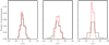 |
Fig. 1 Distribution of the synthetic polarization angles for different simulation models. The black histogram corresponds to observations weighted by density, and the red one without the density weighting. Left: simulation model with MS = 0.7. Middle: simulation model with MS = 2.0. Right: simulation model with MS = 7.0. |
2.2.3 Different f values
Chandrasekhar & Fermi (1953) assumed that “turbulent motions are isotropic”, and they adopted  . If the field strength is weak, turbulent motions will drag the field lines in random directions and turbulence will be isotropic (super-Alfvénic turbulence). However, there is overwhelming observational evidence that magnetic fields in the ISM have well-defined directions, indicating that turbulence is sub, trans-Alfvénic and hence turbulent properties are highly anisotropic (see, for example, Montgomery & Turner 1981; Shebalin et al. 1983; Higdon 1984; Sridhar & Goldreich 1994; Goldreich & Sridhar 1995, 1997). Heyer et al. (2008), using CO data, found that velocity structures in Taurus are highly anisotropic. In the same region, Goldsmith et al. (2008) reported the existence of highly anisotropic density structures, which are aligned parallel to the mean field, known as striations. Striations have also been observed in the Polaris Flare (Panopoulou et al. 2015) and Musca (Cox et al. 2016; Tritsis & Tassis 2018), and they are formed due to magnetosonic waves (Tritsis & Tassis 2016) in sub-Alfvénic turbulence (Beattie & Federrath 2020). More evidence for ordered magnetic fields in molecular clouds can be found in Franco et al. (2010), Franco & Alves (2015), Pillai et al. (2015), Hoq et al. (2017), and Tang et al. (2019). Stephens et al. (2011) explored the magnetic field properties of 52 star forming regions in our Galaxy and concluded that more than 80% of their targets exhibit ordered magnetic fields. The diffuse atomic clouds in our Galaxy are preferentially aligned with the magnetic field (Clark et al. 2014), implying the importance of the magnetic field in their formation. Planck Collaboration Int. XXXV (2016) studied a larger sample of molecular clouds in the Goult Belt and concluded that density structures align parallel or perpendicular to the local mean field direction. This is also consistent with sub, trans-Alfvénic turbulence (e.g., Soler et al. 2013). In addition, Mouschovias et al. (2006), using Zeeman data, concluded that turbulence in molecular clouds is slightly sub-Alfvénic as well. All these lines of evidence indicate that ISM turbulence is sub, trans-Alfvénic, and hence anisotropic.
Other f values were proposed when the DCF method was applied in numerical simulations. Ostriker et al. (2001) performed MHD numerical simulations of giant molecular clouds. They produced synthetic observations and suggested that the DCF equation with f = 0.5 produced accurate measurements for their sub-Alfvénic model. Padoan et al. (2001) simulated protostellar cores and tested the DCF equation in three different cores in a super-Alfvénic MHD turbulent box. They varied the position of the observer with respect to the magnetic field direction and found that, on average, f = 0.4. However, we note that their values range from 0.29 up to 0.74 (see their Table 1). Heitsch et al. (2001) performed 3D MHD simulations of molecular clouds. They found that f lies in the interval 0.33−0.5 (see their Fig. 6) in their three models with strong magnetic fields (sub-Alfvénic turbulence).
In these works, f was found to vary significantly, but a value of f = 0.5 is widely used, for example in Pattle & Fissel (2019). However, no physical connection between f and the turbulent properties of the medium or with specific LOS averaging effects has been demonstrated. Thus, it remains unclear which value of f is most appropriate for any given real physical cloud. The number of turbulent eddies along the LOS may be a relevant metric of f and can be estimated with the HH09 method or following the approach of Cho & Yoo (2016) and Yoon & Cho (2019).
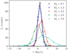 |
Fig. 2 Synthetic emission line profiles for different simulation models. All the models have an Alfvén Mach number MA = 0.7. The sonic Mach number, Ms, for each simulation model is shown in the legend. The dashed lines correspond to the fitted Gaussian profiles. |
2.3 Testing classical DCF with 3D simulations
We tested the DCF method in the 3D numerical simulation we used in Sect. 2.2.2. We created synthetic spectroscopic data following Miville-Deschênes et al. (2003), who assumed optically thin emission and included no chemistry. We set the LOS parallel to the z-axis. We computed the position-position-velocity (PPV) cube,Iv(x, y, v), along the LOS using the following equation,
![Mathematical equation: \begin{equation*}I_{v}(x, y, v)\,{=}\,\sum_{z} \frac{\rho(x, y, z) \delta z}{\sqrt{2\pi} \sigma(x, y, z)} \textrm{exp} \left [ -\frac{ \left (v_{\textrm{los}}(x, y, z) - v \right)^{2} } {2\sigma(x, y, z)^{2}} \right ], \end{equation*}](/articles/aa/full_html/2021/03/aa39779-20/aa39779-20-eq21.png) (13)
(13)
where vlos(x, y, z) is the LOS velocity component, v is the central velocity of each velocity channel, and δz = 1 pixel. The velocity spread is
![Mathematical equation: \begin{equation*} \sigma(x, y, z)\,{=}\,\left [ \left (\frac{\partial v_{\textrm{los}}(x, y, z)}{\partial z} \delta z \right)^{2} + \frac{k_{\textrm{B}}T}{m} \right ]^{1/2}. \end{equation*}](/articles/aa/full_html/2021/03/aa39779-20/aa39779-20-eq22.png) (14)
(14)
In Fig. 2, we show the mean emission profile of each simulation setup derived using Eq. (13). The dots represent the intensity, Iv, versus the gas velocity, and the dashed lines represent the fitted Gaussians. From the fitted Gaussians, we derived the standard deviation of each profile, shown in the σv column of Table 1. In the same table, we show the standard deviation of the polarization angle distribution, δθ, for each setup as well as the estimated Alfvén speed, using the DCF relation (Eq. (5) with f = 1) in the  column. The true Alfvén speed for each setup isshown in the column
  .
.
The DCF method systematically overestimates the magnetic field strength. For the models with Ms = 0.7, the DCF model without an f factor (f = 1) deviates from the true value by a factor of ~5. This impliesthat f needs to equal 1∕5 for the method to produce accurate estimates. On the other hand, for the models with Ms = 1.2, 4.0, and 7.0, the correction factor has to be f ~ 1∕3. It is evident that the generally adopted f = 0.5 value (Sect. 2.2.3) does not apply for these models. Our results indicate that f decreases with Ms, but it remains to be shown whether and why this can be considered a general property.
3 HH09 method
3.1 Foundations of the method
An alternative way to estimate the δB∕B0 ratio was presented by HH09. The method was developed in order to avoid inaccurate estimates of the magnetic field strength induced by sources other than MHD waves, such as large-scale bending of the magnetic field due to gravity and differential rotation. HH09 computed the “isotropic dispersion function” of the polarization map as
![Mathematical equation: \begin{equation*}\left\langle \rm{cos} \left [ \Delta \phi(l) \right ] \right\rangle\,{=}\,\langle \rm{cos} \left [ \Phi(\bm{x}) - \Phi(\bm{x}+\bm{l)} \right ] \rangle. \end{equation*}](/articles/aa/full_html/2021/03/aa39779-20/aa39779-20-eq25.png) (15)
(15)
The quantity Φ(x) denotes the polarization angle measured in radians, x denotes the 2D coordinates in the POS, and l denotes the spatial separation of two polarization measurements in the POS and brackets averaging over the entire polarization map. The polarization angle differences are constrained in the interval [0°, 90°].
HH09 defined the total magnetic field as Btot = B0 + Bt, where B0 is the mean magnetic field component and Bt is the turbulent (or random) component. HH09 assumed that the strength of B0 is uniform and that Bt is induced by gas turbulent motions. They derived the following analytical relation for Eq. (15),
![Mathematical equation: \begin{eqnarray*}1 - \langle \rm{cos} \left [ \Delta \phi (l) \right ] \rangle &\simeq & \sqrt{2\pi} \frac{\langle B_{t}^{2} \rangle}{B_{0}^{2}} \frac{\delta^{3}}{(\delta^{2}+2W^{2})\Delta'}\nonumber\\ &&{\times}\,(1 - e^{l^{2}/2(\delta^{2} + 2W^{2})}) + ml^{2}, \end{eqnarray*}](/articles/aa/full_html/2021/03/aa39779-20/aa39779-20-eq26.png) (16)
(16)
where m is a constant, Δ′ is the effective cloud depth, and W is the beam size. The effective cloud depth is always smaller than the size of the cloud (L), Δ′ ≤ L and is defined as the full width at half maximum (FWHM) of the auto-correlation function of the polarized intensity (Houde et al. 2009). The validity of this relation is limited to spatial scales δ ≤ l ≤ d, where δ is the correlation length of Bt and d is the upper limit below which B0 remains uniform. This equation was used to estimate the  term, which was then inserted into the DCF formula as
![Mathematical equation: \begin{equation*}V^{\rm{DCF+HH09}}_{\textrm{A}} \simeq \sigma_{v} \Bigg [\frac{\langle B_{t}^{2} \rangle^{1/2}}{B_{0}} \Bigg]^{-1}. \end{equation*}](/articles/aa/full_html/2021/03/aa39779-20/aa39779-20-eq28.png) (17)
(17)
The only difference relative to the classical DCF method is that the δB∕B0 term is obtained from the fit of Eq. (16) instead of the dispersion of the polarization angle distribution.
In order to use the method, one has to compute the dispersion function using Eq. (15) and then fit the model in the right hand side of Eq. (16). The fit has the following three free parameters:  , δ, and m.
3.2 Caveats of the method
3.2.1 Omission of the δB ⋅ B0 term
Hildebrand et al. (2009) assumed that “the correlation of Bt and B0 is zero (i.e., ⟨B0 ⋅ Bt⟩ = 0)”, where the averaging is over the full map (see their Eq. (A.2)). We identify three different regimes in which ⟨δB ⋅B0⟩ = 02.
The first is super-Alfvénic turbulence. In the highly super-Alfvénic regime, MHD turbulence behaves like hydro turbulence and δB is random (i.e., ⟨δB⟩ = 0). In this case, B0 is much weaker than δB and the two quantities are statistically independent. Thus,
 (18)
(18)
The second is purely Alfvénic (or incompressible) turbulence. For Alfvénic turbulence, δB ⋅B0 = 0 because Alfvén waves are transverse and their field fluctuations, δB, are always perpendicular to the mean field, B0 (Goldreich & Sridhar 1995).
The third is a force-free field. If we use the linearized (|δB|≪|B0|) induction equation,
 (19)
(19)
where ξ denotes the gas displacements vector, it can be shown that (Spruit 2013)
![Mathematical equation: \begin{equation*}\langle \bm{\delta B} \cdot \bm{B}_{0} \rangle\,{=}\,{-} \frac{1}{4\pi} \int \bm{\xi} \cdot [(\bm{\nabla}\,{\times}\, \bm{B}_{0})\,{\times}\,\bm{B}_{0} ] \textrm{d}V. \end{equation*}](/articles/aa/full_html/2021/03/aa39779-20/aa39779-20-eq32.png) (20)
(20)
If the field isforce-free (i.e., (∇ × B0) × B0 = 0), the above equation implies that ⟨δB ⋅B0⟩ = 0. Although it is occasionally used as an approximation, a force-free field naturally decays without causing fluid motions (Chandrasekhar & Kendall 1957).
The cross-term, ⟨δB ⋅B0⟩, is connected with the compressible modes (Montgomery et al. 1987) for which δB ⋅B0≠0 (Goldreich & Sridhar 1995). Bhattacharjee & Hameiri (1988) and Bhattacharjee et al. (1998), using standard perturbation theory, derived the first-order solution of the equation of motion
 (21)
(21)
where δP3 is the gas-pressure perturbations. The equation of state connects gas density and pressure, and hence
 (22)
(22)
where δρ are the gas density perturbations. Equation (22) explicitly shows the coupling between δρ and δB ⋅B0. Hence, ⟨δB ⋅B0⟩∝⟨δρ⟩, which implies that ⟨δB ⋅B0⟩ = 0 only if ⟨δρ⟩ = 0; this is true for purely incompressible turbulence, which is generally not realizable in the ISM. The omission of the δB ⋅B0 term may lead to significant inaccuracies in the estimate of  when the HH09 method is applied in sub, trans-Alfvénic and compressible turbulence.
3.2.2 Isotropic turbulence
HH09 assumed that “turbulence is isotropic”, and they used a global correlation length, δ. As we argued in Sect. 2.2.3, this goes against observational evidence, which shows highly anisotropic structures and properties. Anisotropic media exhibit different correlation lengths that are perpendicular and parallel to the mean field. This has been shown in the observations of Higdon (1984) and Heyer et al. (2008) as well as by numerous theoretical works, such as Shebalin et al. (1983), Goldreich & Sridhar (1995), Sridhar & Goldreich (1994), Cho & Vishniac (2000), and Maron & Goldreich (2001) (see Oughton & Matthaeus 2020, for a recent review). This indicates that anisotropic structure functions, similar to those in Cho & Vishniac (2000) and Maron & Goldreich (2001), should be used instead. Chitsazzadeh et al. (2012) and Houde et al. (2013) refined the HH09 method and considered the anisotropic turbulent properties of sub, trans-Alfvénic turbulence. Our criticism, however, focuses on the original isotropic version of the method, which is often still applied (e.g., Chuss et al. 2019).
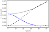 |
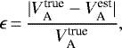
Fig. 3 Dispersion function of the synthetic polarization map. Black dots correspond to the dispersion function computed using Eq. (15) for the Ms = 0.7 model. The model fit at large scales is shown with the broken dashed curve. Blue points mark the dispersion function subtracted with the dashed black line, and the blue line shows the fit of Eq. (23). |
3.2.3 Sparsity of data and the HH09 method
The computation of the dispersion function (Eq. (15)) for sparsely sampled data introduces a bias. Soler et al. (2016) showed that the dispersion function computed with optical polarization is slightly different than the one computed with submillimeter data (see their Fig. 6). They commented that the sparse sampling of the optical polarization measurements induces a “jittering.” Their figures indicate that the structure function with the optical data systematically overestimates the intercept of the function. As a result, for the case of the sparse sampling, the  parameter would be biased toward higher values. No solution to this problem has been suggested yet.
3.3 Testing HH09 with 3D simulations
We applied the HH09 method to the polarization angle maps, χ(x, y), that we created in Sect. 2.2.2, as suggested by Houde et al. (2009). We computed the dispersion function (Eq. (15)) from our synthetic data (black dots in Fig. 3). We then fit the right-hand side of Eq. (16) to the black dots without including the exponential term. This fit, shown with the black broken curve, was performed at larger scales (i.e., l > 20 pixels). The dashed black curve is then subtracted from the black points and the result, shown with the blue dots, corresponds to the turbulent auto-correlation function, that is, to the second term of Eq. (16),
 (23)
(23)
We fit this term to the blue points and derived the turbulent correlation length (dashed blue curve in Fig. 3), δ. The turbulent-to-ordered magnetic field ratio is
 (24)
(24)
where N is the number of turbulent cells along the LOS and is defined as
 (25)
(25)
where Δ′ is computed as in Houde et al. (2009). Similar to in the optical polarization data, the beam resolution is infinite in our synthetic observations, and hence W = 0 (Franco et al. 2010; Panopoulou et al. 2016). In Appendix A, we show the dispersion function plots for the rest of the models, and the best-fit parameters are given in Table A.1.
The turbulent-to-ordered ratio obtained for the different simulation models is shown in column  of Table 1. The estimated Alfvén speed when the HH09 method is combined with the DCF method is shown in the
  column of the same table. The DCF+HH09 estimates are significantly improved compared to the classical DCF values, although the overestimation from the true Alfvén speed (
 ) is still prominent. We note, however, that if we consider the effective cloud depth to be equal to the cloud size (i.e., Δ′ = 256 pixels), the HH09 method produces more accurate estimates of the field strength for the models with Ms = 4.0 and 7.0.
4 Proposed method
Motivated by the existence of compressible modes and the contamination they induce in the aforementioned methods, we propose a generalized method that takes these modes into account. We started with Eq. (1). Similar to DCF, we assumed that gas is perfectly attached to the magnetic field and that turbulent motions are completely transferred to magnetic fluctuations. Unlike DCF, “we assumed that all MHD modes are excited, including fast and slow modes”. Since we included the compressible modes, we did not omit the cross-term in the magnetic energy, which for the general case is δB ⋅B0≠0 (see Sect. 3.2.1). To leading order, the fluctuating part in the energy equation, when |δB |≪|B0|, will be (Federrath 2016)
 (26)
(26)
The above equation implies that δB is aligned with B0. This can be understood due to the local alignment between δB and δv, which appears in sub-Alfvénic turbulence (Boldyrev 2005). This is known as “dynamic alignment” and has been observed in numerical simulations of both incompressible (e.g., Mason et al. 2006) and compressible (e.g., Kritsuk et al. 2017) turbulence. Velocity gradients parallel to B0, which only appear in compressible turbulence, drag δB to align with B0 (Beattie et al. 2020) due to the dynamic alignment. Despite its simplicity, the accuracy of Eq. (26) was proven to be remarkable when tested in numerical simulations of sub-Alfvénic and compressible turbulence (Federrath 2016; Beattie et al. 2020). We assumed that turbulent kinetic energy is equal to magnetic energy fluctuations, and hence
 (27)
(27)
As in the DCF method, we used the relation δθ = δB∕B0 since the turbulent-to-ordered ratio is measured from the polarization angle distribution. We obtained
 (28)
(28)
which can be solved for the Alfvén speed,  , as
, as
 (29)
(29)
As in DCF, we assumed that there is a guiding field around which MHD waves propagate. We also assumed that turbulent kinetic energy is equal to the fluctuating magnetic energy, “which is given by δBB0, since it is the dominant (first-order) term in the magnetic energy”. This term was neglected in previous methods. The major difference between our equation and the DCF equation is that the  term in our equation appears with n = −1∕2, while in DCF it is n = −1.
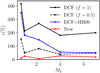 |
Fig. 4 Relative deviation of each method estimate for the different simulation models. All the models have MA = 0.7. |
4.1 Testing the proposed method with 3D simulations
We applied the proposed method to the 3D compressible MHD simulations (see Sect. 2.2.2) in order to test its validity. We used the δθ and σv from Table 1. In the  column of the same table, we show the value computed using Eq. (29). It is evident that our model produces acceptably accurate estimates of the true VA in all models.
The relative deviation of the estimated VA from the true oneis
 (30)
(30)
where  is the true VA and
  is the estimated value from the various methods. In Fig. 4, we show ϵ(%) for all models. The black points correspond to the DCF method with f = 1 (solid line) and f = 0.5 (dotted line), the blue points correspond to HH09, and the red points correspond to the new proposed method (Eq. (29)). The DCF method systematically overestimates the true value, and, even with the previously reported two-fold reduction (i.e., f = 0.5), the deviations are still significant. Combining the DCF and HH09 methods produces very large estimates in the models with low Ms, while at higher Ms the method is more accurate. Our proposed method produces quite accurate values for the field strength regardless of the value of Ms. The mean deviation, ϵ, of our method is 17%. The largest deviation is seen in the model with Ms = 4.0, where ϵ = 27%.
Although the accuracy of our method does not depend on Ms, our method systematically underestimates the true field strength. This can be explained by the non-homogeneity effect that we discussed in Sect. 2.2.2. The polarization map includes dispersion due to density enhancements, and hence δθ overestimates the δB∕B0 ratio. Only in the model with Ms = 0.7, where density inhomogeneities are minimal, does the method slightly overestimate the field strength.
4.2 Limitations of our method
There are limitations of our method related to the observables and the physics behind the proposed equation. Firstly, polarization angle maps are affected by density inhomogeneities, and hence they do not probe the δB∕B0 term accurately. The observed spread is higher than the true ratio, and hence the field strength is underestimated. This non-homogeneity effect is the dominant uncertainty in our method. Secondly, as in the DCF method, we neglected the contribution of self-gravity. In the presence of self-gravity, the field lines are bent and the observed δθ and δv are higher. Other methods have to be employed prior to ours (e.g., the Girart et al. 2006 and Pattle et al. 2017 methods) in order to remove the self-gravity effects from both polarization and spectroscopic maps.
Finally, not all the MHD modes induce δB∕B0 variations. For example, for very strong fields, fast modes can propagate perpendicularly to the mean field and oscillate like a harmonica without disturbing the field lines. These modes will contribute to the velocity, but not the polarization angle, biasing the magnetic field estimate to higher values. The tests we performed, however, show that this is not a very important effect.
5 Discussion and conclusions
Dust polarization traces the magnetic field orientation in the POS, but not its strength. DCF and HH09 are the most widely applied methods that employ polarization data in order to estimate the strength of the field. They rely on the assumption that isotropic gas turbulence motions induce the propagation of small amplitude Alfvén waves, |δB |≪|B0|. Observations indicate that turbulence in the ISM is highly anisotropic (e.g., Higdon 1984; Heyer et al. 2008; Planck Collaboration Int. XXXV 2016; see also Sect. 2.2.3). The sufficiently high Ms in the ISM (Heiles & Troland 2003) implies that compressible modes are important. Both the DCF and HH09 methods neglect the compressible modes. As a result, the estimates of the magnetic field they provide may deviate significantly from the true value.
We tested the DCF method in synthetic observations from publicly available 3D MHD simulations. We found that the DCF method systematically overestimates the true strength value. The previously reported reduction factor, f = 0.5, is not supported by our analysis. We found similar results when we tested the HH09 method. However, the accuracy of the HH09 method improves significantly for models with high sound Mach numbers.
We proposed a new method to estimate the magnetic field strength in the ISM. We accounted for all MHD modes, both Alfvén andcompressible. We assumed that: wave fluctuations are sufficiently small compared to the mean field strength, |δB |≪|B0|; turbulent kinetic energy is equal to the fluctuating part of the magnetic energy density; and the fluctuating magnetic energy is dominated by the δBB0 cross-term, which represents the compressible modes. Instead of
 (31)
(31)
we proposed the following equation:
 (32)
(32)
where ρ is the gas density, δv is the spread in spectroscopic data emission lines, and δθ is the dispersion of polarization angles.
We tested the validity of our equation in synthetic observations, and we compared its accuracy to that of the classical DCF method as well as to that of the combined DCF and HH09 method. Our method outperforms these methods and guarantees a uniformly low error independent of Mach number and “without the need for a correction factor”.
Acknowledgements
This work is dedicated to the memory of Roger Hildebrand, a pioneer in this field and an inspiring mentor. We are grateful to the referee M. Houde for his careful and constructive reviewing. R.S. would like to thank J. Beattie and A. Tsouros for productive discussions and Dr. B. Burkhart for her help with their numerical simulations. We thank A. Tritsis for his invaluable comments. We also thank N. D. Kylafis for his careful reading of the manuscript, V. Pavlidou and G. V. Panopoulou for fruitful discussions. R.S. would like to thank Dr. K. Christidis for his constant support during this project. This project has received funding from the European Research Council (ERC) under the European Unions Horizon 2020 research and innovation programme under grant agreement No. 771282.
Appendix A Dispersion function fitting
The dispersion function fits for the models with Ms = 1.2−7.0 are shown in Fig. A.1. The best-fit parameters for each model are given in Table A.1.
Fitting parameters of the HH09 method.
References
- Andersson, B. G., Lazarian, A., & Vaillancourt, J. E. 2015, ARA&A, 53, 501 [NASA ADS] [CrossRef] [Google Scholar]
- Beattie, J. R., & Federrath, C. 2020, MNRAS, 492, 668 [Google Scholar]
- Beattie, J. R., Federrath, C., & Seta, A. 2020, MNRAS, 498, 1593 [Google Scholar]
- Bhattacharjee, A., & Hameiri, E. 1988, Phys. Fluids, 31, 1153 [Google Scholar]
- Bhattacharjee, A., Ng, C. S., & Spangler, S. R. 1998, ApJ, 494, 409 [NASA ADS] [CrossRef] [Google Scholar]
- Bialy, S., & Burkhart, B. 2020, ApJ, 894, L2 [CrossRef] [Google Scholar]
- Boldyrev, S. 2005, ApJ, 626, L37 [NASA ADS] [CrossRef] [Google Scholar]
- Burkhart, B., Falceta-Gonçalves, D., Kowal, G., & Lazarian, A. 2009, ApJ, 693, 250 [NASA ADS] [CrossRef] [Google Scholar]
- Burkhart, B., Appel, S. M., Bialy, S., et al. 2020, ApJ, 905, 14 [Google Scholar]
- Chandrasekhar, S., & Fermi, E. 1953, ApJ, 118, 113 [NASA ADS] [CrossRef] [Google Scholar]
- Chandrasekhar, S., & Kendall, P. C. 1957, ApJ, 126, 457 [NASA ADS] [CrossRef] [Google Scholar]
- Chitsazzadeh, S., Houde, M., Hildebrand, R. H., & Vaillancourt, J. 2012, ApJ, 749, 45 [Google Scholar]
- Cho, J., & Lazarian, A. 2002, Phys. Rev. Lett., 88, 245001 [Google Scholar]
- Cho, J., & Lazarian, A. 2003, MNRAS, 345, 325 [NASA ADS] [CrossRef] [Google Scholar]
- Cho, J.„ & Vishniac, E. T. 2000, ApJ, 538, 217 [NASA ADS] [CrossRef] [Google Scholar]
- Cho, J., & Yoo, H. 2016, ApJ, 821, 21 [NASA ADS] [CrossRef] [Google Scholar]
- Chuss, D. T., Andersson, B. G., Bally, J., et al. 2019, ApJ, 872, 187 [NASA ADS] [CrossRef] [Google Scholar]
- Clark, S. E., Peek, J. E. G., & Putman, M. E. 2014, ApJ, 789, 82 [Google Scholar]
- Cox, N. L. J., Arzoumanian, D., André, P., et al. 2016, A&A, 590, A110 [NASA ADS] [CrossRef] [EDP Sciences] [Google Scholar]
- Davis, L. 1951, Phys. Rev., 81, 890 [NASA ADS] [CrossRef] [PubMed] [Google Scholar]
- Falceta-Gonçalves, D., Lazarian, A., & Kowal, G. 2008, ApJ, 679, 537 [NASA ADS] [CrossRef] [Google Scholar]
- Federrath, C. 2016, J. Plasma Phys., 82, 535820601 [CrossRef] [Google Scholar]
- Franco, G. A. P., & Alves, F. O. 2015, ApJ, 807, 5 [NASA ADS] [CrossRef] [Google Scholar]
- Franco, G. A. P., Alves, F. O., & Girart, J. M. 2010, ApJ, 723, 146 [Google Scholar]
- Girart, J. M., Rao, R., & Marrone, D. P. 2006, Science, 313, 812 [NASA ADS] [CrossRef] [PubMed] [Google Scholar]
- Goldreich, P., & Sridhar, S. 1995, ApJ, 438, 763 [NASA ADS] [CrossRef] [Google Scholar]
- Goldreich, P., & Sridhar, S. 1997, ApJ, 485, 680 [NASA ADS] [CrossRef] [Google Scholar]
- Goldsmith, P. F., Heyer, M., Narayanan, G., et al. 2008, ApJ, 680, 428 [NASA ADS] [CrossRef] [Google Scholar]
- Heiles, C., & Troland, T. H. 2003, ApJS, 145, 329 [NASA ADS] [CrossRef] [Google Scholar]
- Heitsch, F., Zweibel, E. G., Mac Low, M.-M., Li, P., & Norman, M. L. 2001, ApJ, 561, 800 [NASA ADS] [CrossRef] [Google Scholar]
- Hensley, B. S., Zhang, C., & Bock, J. J. 2019, ApJ, 887, 159 [Google Scholar]
- Heyer, M., Gong, H., Ostriker, E., & Brunt, C. 2008, ApJ, 680, 420 [NASA ADS] [CrossRef] [Google Scholar]
- Heyvaerts, J., & Priest, E. R. 1983, A&A, 117, 220 [NASA ADS] [Google Scholar]
- Higdon, J. C. 1984, ApJ, 285, 109 [NASA ADS] [CrossRef] [Google Scholar]
- Hildebrand, R. H., Kirby, L., Dotson, J. L., Houde, M., & Vaillancourt, J. E. 2009, ApJ, 696, 567 [NASA ADS] [CrossRef] [Google Scholar]
- Hill, A. S., Benjamin, R. A., Kowal, G., et al. 2008, ApJ, 686, 363 [NASA ADS] [CrossRef] [Google Scholar]
- Hoq, S., Clemens, D. P., Guzmán, A. E., & Cashman, L. R. 2017, ApJ, 836, 199 [NASA ADS] [CrossRef] [Google Scholar]
- Houde, M. 2004, ApJ, 616, L111 [Google Scholar]
- Houde, M., Vaillancourt, J. E., Hildebrand, R. H., Chitsazzadeh, S., & Kirby, L. 2009, ApJ, 706, 1504 [NASA ADS] [CrossRef] [Google Scholar]
- Houde, M., Fletcher, A., Beck, R., et al. 2013, ApJ, 766, 49 [NASA ADS] [CrossRef] [Google Scholar]
- Hull, C. L. H., & Zhang, Q. 2019, Front. Astron. Space Sci., 6, 3 [NASA ADS] [CrossRef] [Google Scholar]
- Kritsuk, A. G., Ustyugov, S. D., & Norman, M. L. 2017, New J. Phys., 19, 065003 [CrossRef] [Google Scholar]
- Kudoh, T., & Basu, S. 2003, ApJ, 595, 842 [NASA ADS] [CrossRef] [Google Scholar]
- Lazarian, A., Yuen, K. H., & Pogosyan, D. 2020, ApJ, submitted [Google Scholar]
- Lee, H. M., & Draine, B. T. 1985, ApJ, 290, 211 [NASA ADS] [CrossRef] [Google Scholar]
- Lithwick, Y., & Goldreich, P. 2001, ApJ, 562, 279 [NASA ADS] [CrossRef] [Google Scholar]
- Maron, J., & Goldreich, P. 2001, ApJ, 554, 1175 [NASA ADS] [CrossRef] [Google Scholar]
- Mason, J., Cattaneo, F., & Boldyrev, S. 2006, Phys. Rev. Lett., 97, 255002 [NASA ADS] [CrossRef] [PubMed] [Google Scholar]
- Miville-Deschênes, M. A., Levrier, F., & Falgarone, E. 2003, ApJ, 593, 831 [NASA ADS] [CrossRef] [Google Scholar]
- Montgomery, D., & Turner, L. 1981, Phys. Fluids, 24, 825 [NASA ADS] [CrossRef] [Google Scholar]
- Montgomery, D., Brown, M. R., & Matthaeus, W. H. 1987, J. Geophys. Res., 92, 282 [NASA ADS] [CrossRef] [Google Scholar]
- Mouschovias, T. C., Tassis, K., & Kunz, M. W. 2006, ApJ, 646, 1043 [NASA ADS] [CrossRef] [Google Scholar]
- Myers, P. C., & Goodman, A. A. 1991, ApJ, 373, 509 [NASA ADS] [CrossRef] [Google Scholar]
- Ostriker, E. C., Stone, J. M., & Gammie, C. F. 2001, ApJ, 546, 980 [NASA ADS] [CrossRef] [Google Scholar]
- Oughton, S., & Matthaeus, W. H. 2020, ApJ, 897, 37 [Google Scholar]
- Padoan, P., Goodman, A., Draine, B. T., et al. 2001, ApJ, 559, 1005 [NASA ADS] [CrossRef] [Google Scholar]
- Panopoulou, G., Tassis, K., Blinov, D., et al. 2015, MNRAS, 452, 715 [Google Scholar]
- Panopoulou, G. V., Psaradaki, I., & Tassis, K. 2016, MNRAS, 462, 1517 [NASA ADS] [CrossRef] [Google Scholar]
- Pattle, K., & Fissel, L. 2019, Front. Astron. Space Sci., 6, 15 [CrossRef] [Google Scholar]
- Pattle, K., Ward-Thompson, D., Berry, D., et al. 2017, ApJ, 846, 122 [NASA ADS] [CrossRef] [Google Scholar]
- Pillai, T., Kauffmann, J., Tan, J. C., et al. 2015, ApJ, 799, 74 [NASA ADS] [CrossRef] [Google Scholar]
- Planck Collaboration Int. XXXV. 2016, A&A, 586, A138 [NASA ADS] [CrossRef] [EDP Sciences] [Google Scholar]
- Portillo, S. K. N., Slepian, Z., Burkhart, B., Kahraman, S., & Finkbeiner, D. P. 2018, ApJ, 862, 119 [Google Scholar]
- Shebalin, J. V., Matthaeus, W. H., & Montgomery, D. 1983, J. Plasma Phys., 29, 525 [NASA ADS] [CrossRef] [Google Scholar]
- Soler, J. D., Hennebelle, P., Martin, P. G., et al. 2013, ApJ, 774, 128 [NASA ADS] [CrossRef] [Google Scholar]
- Soler, J. D., Alves, F., Boulanger, F., et al. 2016, A&A, 596, A93 [NASA ADS] [CrossRef] [EDP Sciences] [Google Scholar]
- Spruit, H. C. 2013, arXiv e-prints [arXiv:1301.5572] [Google Scholar]
- Sridhar, S., & Goldreich, P. 1994, ApJ, 432, 612 [NASA ADS] [CrossRef] [Google Scholar]
- Stephens, I. W., Looney, L. W., Dowell, C. D., Vaillancourt, J. E., & Tassis, K. 2011, ApJ, 728, 99 [NASA ADS] [CrossRef] [Google Scholar]
- Tang, Y.-W., Koch, P. M., Peretto, N., et al. 2019, ApJ, 878, 10 [CrossRef] [Google Scholar]
- Tritsis, A., & Tassis, K. 2016, MNRAS, 462, 3602 [CrossRef] [Google Scholar]
- Tritsis, A., & Tassis, K. 2018, Science, 360, 635 [NASA ADS] [CrossRef] [Google Scholar]
- Wiebe, D. S., & Watson, W. D. 2004, ApJ, 615, 300 [Google Scholar]
- Yoon, H., & Cho, J. 2019, ApJ, 880, 137 [Google Scholar]
- Zweibel, E. G. 1990, ApJ, 362, 545 [NASA ADS] [CrossRef] [Google Scholar]
We use the more general notation δB instead of Bt since it refers to the fluctuating component of the magnetic field, which is not necessarily in turbulent conditions.
Bhattacharjee & Hameiri (1988) and Bhattacharjee et al. (1998) used the subscript 1 instead of δ for the perturbed quantities.
All Tables
All Figures
|
Fig. 1 Distribution of the synthetic polarization angles for different simulation models. The black histogram corresponds to observations weighted by density, and the red one without the density weighting. Left: simulation model with MS = 0.7. Middle: simulation model with MS = 2.0. Right: simulation model with MS = 7.0. |
| In the text | |
|
Fig. 2 Synthetic emission line profiles for different simulation models. All the models have an Alfvén Mach number MA = 0.7. The sonic Mach number, Ms, for each simulation model is shown in the legend. The dashed lines correspond to the fitted Gaussian profiles. |
| In the text | |
|
Fig. 3 Dispersion function of the synthetic polarization map. Black dots correspond to the dispersion function computed using Eq. (15) for the Ms = 0.7 model. The model fit at large scales is shown with the broken dashed curve. Blue points mark the dispersion function subtracted with the dashed black line, and the blue line shows the fit of Eq. (23). |
| In the text | |
|
Fig. 4 Relative deviation of each method estimate for the different simulation models. All the models have MA = 0.7. |
| In the text | |
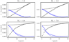 |
Fig. A.1 As in Fig. 3 but for the simulation models with Ms = 1.2−7.0. |
| In the text | |
Current usage metrics show cumulative count of Article Views (full-text article views including HTML views, PDF and ePub downloads, according to the available data) and Abstracts Views on Vision4Press platform.
Data correspond to usage on the plateform after 2015. The current usage metrics is available 48-96 hours after online publication and is updated daily on week days.
Initial download of the metrics may take a while.