| Issue |
A&A
Volume 647, March 2021
|
|
|---|---|---|
| Article Number | A75 | |
| Number of page(s) | 12 | |
| Section | Astrophysical processes | |
| DOI | https://doi.org/10.1051/0004-6361/202039088 | |
| Published online | 10 March 2021 | |
Stellar wind structures in the eclipsing binary system IGR J18027–2016
1
Instituto Argentino de Radioastronomía (CCT-La Plata, CONICET; CICPBA; UNLP), C.C. No. 5, 1894 Villa Elisa, Argentina
e-mail: This email address is being protected from spambots. You need JavaScript enabled to view it.
2
Facultad de Ciencias Astronómicas y Geofísicas, Universidad Nacional de La Plata, Paseo del Bosque s/n, 1900 La Plata, Argentina
3
Kapteyn Astronomical Institute, University of Groningen, PO BOX 800, 9700 AV Groningen, The Netherlands
4
AIM, CEA, CNRS, Université Paris-Saclay, Université de Paris, 91191 Gif-sur-Yvette, France
5
Université de Paris, CNRS, Astroparticule et Cosmologie, 75013 Paris, France
Received:
2
August
2020
Accepted:
16
December
2020
Abstract
Context. IGR J18027–2016 is an obscured high-mass X-ray binary formed by a neutron star accreting from the wind of a supergiant companion with a ∼4.57 d orbital period. The source shows an asymmetric eclipse profile that remained stable across several years.
Aims. We aim to investigate the geometrical and physical properties of stellar wind structures formed by the interaction between the compact object and the supergiant star.
Methods. In this work we analysed the temporal and spectral evolution of this source along its orbit using six archival XMM-Newton observations and the accumulated Swift/BAT hard X-ray light curve.
Results. The XMM-Newton light curves show that the source hardens during the ingress and egress of the eclipse, in accordance with the asymmetric profile seen in Swift/BAT data. A reduced pulse modulation is observed on the ingress to the eclipse. We modelled XMM-Newton spectra by means of a thermally Comptonized continuum (NTHCOMP), adding two Gaussian emission lines corresponding to Fe Kα and Fe Kβ. We included two absorption components to account for the interstellar and intrinsic media. We found that the local absorption column outside the eclipse fluctuates uniformly around ∼6 × 1022 cm−2, whereas when the source enters and leaves the eclipse the column increases by a factor of ≳3, reaching values up to ∼35 and ∼15 × 1022 cm−2, respectively.
Conclusions. Combining the physical properties derived from the spectral analysis, we propose a scenario in which, primarily, a photo-ionisation wake and, secondarily, an accretion wake are responsible for the orbital evolution of the absorption column, continuum emission, and variability seen at the Fe-line complex.
Key words: X-rays: binaries / X-rays: individuals: IGR J18027–2016 / stars: neutron
© ESO 2021
1. Introduction
Since its launch in 2002, the Soft Gamma-Ray Imager (IBIS/ISGRI) detector (Lebrun et al. 2003; Ubertini et al. 2003) on board the INTEGRAL observatory (Winkler et al. 2003) has discovered a large number of hard and obscured X-ray sources.
Most of these sources have a Galactic origin and belong to the class of high-mass X-ray binaries (HMXB). Based on the spectral type of the companion star (mainly seen in optical), the accretion mechanisms taking place, and their X-ray behaviour, HMXBs are further classified into Be (later called BeXBs) or supergiant X-ray binaries (SgXBs). In Be systems, the compact object (CO) is mainly a neutron star (NS) with moderately eccentric orbits (P ∼ 10–100 d) and spends short time intervals in close proximity to the dense circumstellar disc surrounding the Be companion (Negueruela & Coe 2002; Liu et al. 2000). In SgXBs, the COs are typically in shorter (1–10 d) orbits around an OB supergiant companion. In those systems, accretion can be driven by Roche lobe overflow and/or through the powerful supergiant stellar wind (for a review, see e.g., Chaty 2013).
In this last category, two sub-classes of binary systems appear. The first usually exhibits high levels of obscuration (NH ∼ 1023 − 1024 cm−2) that is local to the source (Walter et al. 2006; Chaty et al. 2008). The second is composed of binary systems consisting of COs associated with a supergiant donor that undergoes fast transient outbursts in the X-ray band. These latter sources are called supergiant fast X-ray transients (SFXT; Negueruela et al. 2006; Sguera et al. 2006).
The obscured source IGR J18027–2016 is a typical SgXB, which was discovered during the first year of operations by INTEGRAL. The source was spatially associated with the X-ray pulsar SAX J1802.7–2017 by Augello et al. (2003). Later on, Hill et al. (2005) reported that the source is an eclipsing HMXB system composed of an accreting X-ray pulsar and a late OB supergiant star that has persistent emission and high intrinsic photoelectric absorption. Timing analysis performed on the ISGRI data by these authors confirmed the nature of the source and constrained its orbital period to Porb = 4.5696 ± 0.0009 d with a mid-eclipse ephemeris at Tmid = 52931.37 ± 0.04 MJD.
The near-infrared (NIR) counterpart (2MASS J18024194–2017172) of this source was identified by Masetti et al. (2008). These authors obtained a low-resolution optical spectrum and showed that it is a very reddened early-type star. Using the mass and radius deduced by Hill et al. (2005), they argued that the counterpart should be a B-type giant. Later, Chaty et al. (2008) confirmed the identification of the counterpart. Based on the R⋆/D⋆ value of the normalization that minimizes χ2 on the black-body SED fitting to the optical as well as the NIR and mid-infrared (MIR) data, and assuming a typical B-star radius of R⋆ = 20 R⊙, Torrejón et al. (2010) estimated a distance to the source of D⋆= 12.4 ± 0.1 kpc within a 90% confidence level.
Using Swift/BAT and ISGRI/INTEGRAL data, Coley et al. (2015) and Falanga et al. (2015) independently provided better constraints to IGR J18027–2016 parameters such as orbital period and eclipsing phases. They also proposed various mechanisms that may be responsible for creating an asymmetric eclipse profile, including large stellar wind structures (such as accretion wakes and photo-ionization wakes) and non-zero eccentricity orbits (0.04 < e < 0.2). Aftab et al. (2019) and Pradhan et al. (2019) studied the orbital behaviour of IGR J18027–2016 using Swift/BAT and XMM-Newton data from a different perspective; they concluded that stellar wind clumps may be responsible for the short- and long-term variability and spectral behaviour of the source.
In this paper, we present a detailed temporal and spectral analysis of all publicly available XMM-Newton and Swift/BAT observations (same data set as Pradhan et al. 2019) to investigate the behaviour of the X-ray emission of IGR J18027–2016 along the orbital revolution of the system. In our approach, we consider and treat in particular the strong background and pile-up that affects half of the XMM-Newton observations. In Sect. 2, we provide information on the observations and data reduction methods employed for the analysis. We describe the results of our temporal and spectral X-ray analysis in Sect. 3. In Sect. 4 we discuss our results and introduce a possible astrophysical scenario to describe the temporal and spectral orbital variability of the system. Finally, a summary of all the obtained results is presented in Sect. 5.
2. Observations and data reduction
2.1. XMM-Newton data
The XMM-Newton observatory contains two X-ray instruments: the European Photon Imaging Camera (EPIC) and the Reflecting Grating Spectrometers (RGS). The EPIC instrument is comprised of three detectors, a PN camera (Strüder et al. 2001), and two MOS cameras (Turner et al. 2001), which all operate in the 0.3–12 keV energy range. The RGS consists of two high-resolution spectrometers sensitive in the 0.3–2.0 keV soft energy range.
XMM-Newton first pointed at IGR J18027–2016 on April 06, 2004 (PI: R. Walter) and then five more times between September 06 and September 13, 2014 (PI: A. Manousakis). The first observation was performed with a medium filter in large window mode, while the rest of the exposures were conducted with a medium filter in full frame observation mode. As RGS only covers the highly absorbed soft band up to ∼2.0 keV, we were prevented from using those spectrometers in our analysis, given the highly obscured nature of IGR J18027–2016. For our analysis, we started considering PN and MOS cameras; however, because of the larger integration time of MOS cameras and the presence of pile–up (see below), in what follows we only consider the PN camera.
We reduced the XMM-Newton data using the Science Analysis System (SAS) version 18.0.0 and the latest calibrations available by February 2019. By processing the observation data files (ODF) with the EPPROC task we produced event lists from the PN data sets. Basic information on the six observations used in this work is given in Table 1.
XMM-Newton PN observations used in this work.
In order to exclude high-background periods and generate good-time intervals (GTI) we produced light curves of 100 s bin excluding the entire CCD (CCDNR!=4) in which the bright IGR J18027–2016 source is located. For these we only considered events with energies in the 10–12 keV range.
Some of the PN exposures were heavily affected by high background activity. In such cases, following the standard GTI procedure (rate < 0.4 counts per second, or cps), the effective exposure times were strongly reduced, which avoided further scientific analysis. In particular, for the observation covering the eclipse (#74), from the total ∼40 ks of exposure time, only 7% is retained after filtering. This particular example is shown in Fig. 1. The entire collection of background light curves can be found in Fig. A.1 in the on-line version of this work.
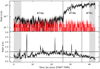 |
Fig. 1. Source and background light curves of the eclipse observation #74 using 100 s bins. Top panel: source+background (black) and background (red) light curves extracted in the 0.5–12 keV energy range using circular regions with equal area. Bottom panel: full CCD light curve in the 10–12 keV energy range excluding the source region. The black vertical lines indicate split times for eclipse (a), egress (b), and out-of-eclipse (c) periods, according to (Coley et al. 2015) ephemeris. The full (dashed) horizontal line corresponds to the background rate of 1 cps (0.4 cps). |
The top panel of Fig. 1 shows the source-plus-background and background only light curves at 0.5–12 keV (100 s bin) for different circular regions of the same radius (600 physical units, or PhU). The bottom panel shows the full-CCD background light curve in the 10–12 keV (100 s bin) energy range, excluding the source region. When following the standard cut-out rate of 0.4 cps, only a small portion of the first and last 3 ks remains in the GTI. Thus, in such a case, the full information associated with the eclipse and its egress would be lost. Taking into account the high count rate exhibited by the source in all the observations, we decided to increase the standard rate limit for GTIs to 1 cps to minimize the issue raised by the presence of the background. With this new limit, bright and fast background flares are still excluded, while the exposure times for science are highly increased, and the background count rate in the 0.5–12 keV energy range for a region with the same area as the source extraction region is negligible with respect to the source events (see red light curve in Fig. 1).
In Table 1 we present the remaining exposure times (in kiloseconds) of each observation, according to the chosen background rate limit. One column shows the GTIs for the standard rate of 0.4 cps while the second column corresponds to the selected limit of 1 cps. To be conservative we used the increased rate limit only for eclipse observation #74.
To check for pile-up effects, we used the SAS task EPATPLOT to create diagnoses of the relative ratios of single- (PATTERN==0) and double- (PATTERN IN [1:4]) events and to study their deviations from the expected calibrated values. Using a circular region of 600 PhU centred at the source and 0.5–12 keV energy range (PILEUPNUMBERENERGYRANGE), we found that three of the six observations were affected by pile-up.
For each of the observations showing pile-up we produced new EPATPLOTS extracting events from a series of annuli varying the inner radius of the PSF by 10, 20, 30, etcetera PhU, with a fixed outer radius of 600 PhU. We then searched for the minimum excision inner radius in which the pattern coefficients for single and double (reported on the EPATPLOTS) were consistent with unity within errors. In the last column of Table 1, we show the excision radii considered for each of the observations.
We note that, in contrast, Pradhan et al. (2019) mention that the high-energy background above the standard count rate limit only affected observation #26 and that none of the observations were affected by pile-up. A strict comparison is odd owing to the absence of detailed information on the background treatment. Both light curves and spectra might be affected by background and pile-up effects.
2.2. Swift/BAT data
The Swift/Burst Alert Telescope (BAT) is an X-ray instrument working in the 15–50 keV energy range, which provides almost real-time monitoring of the hard X-ray sky. The BAT covers ∼90% of the sky each day reaching full-day detection sensitivities of 5.3 mCrab, at a temporal resolution of 64 s (Krimm et al. 2013).
In this paper we consider the full daily light curve of IGR J18027–2016 available up to February 14, 2019 in the Swift/BAT service1, a public website where more than 900 light curves of hard X-ray sources are available, spanning for more than eight years.
3. Results
3.1. X-ray light curves
3.1.1. Swift/BAT
After retrieving the full light curve, we created the orbital-period folded light curve using 50 phase bins based on the refined ephemeris of Coley et al. (2015) (Porb = 4.56993 d and Tmid = 55083.82 BMJD). In this paper we consider the mid-eclipse phase to be ϕ = 0.
In Fig. 2 we can clearly identify the eclipsing-binary nature of the source, where the eclipse spans for ∼20% of the entire cycle. Moreover, we also note that the transition into the eclipse is more gradual than the eclipse egress. This corresponds to the asymmetry on the eclipse profile already studied by Coley et al. (2015) and Falanga et al. (2015).
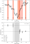 |
Fig. 2. Top: folded Swift/BAT daily light curve using 32 phase bins with a period of 4.56993 d and mid-eclipse reference time of 55083.82 BMJD (Coley et al. 2015). The vertical light red stripes correspond to the six XMM-Newton observations used in this paper with their widths representing their final exposure times after GTI filtering. Bottom: neutron star spin periods for each observation, estimated by fitting a Lorentzian profile to the χ2 distribution of the period search. Observation #74a (eclipse) was not included in the analysis. Average spin periods of 140.015 ± 0.0008 s and 139.81 ± 0.02 s before and after the eclipse, respectively, are registered (excluding Obs #26, as it corresponds to a different epoch). Averages are indicated with dashed lines. |
3.1.2. XMM-Newton
We extracted PN light curves using EVSELECT task from SAS using 1, 10, 50, and 100 s bin sizes for a source region of 30 arcsec (600 PhU). For the background region, we used another circular region of 30 arcsec on the same chip as the source, following XMM-Newton technical recommendations2. Background substraction was made by means of EPICLCCORR task from SAS. Light curves were extracted on three energy bands: soft: 0.5–6 keV, hard: 6–12 keV, and full: 0.5–12 keV for timing analysis and on 0.5–6.1 keV, 6.1–6.7 keV, and 6.7–12 keV for further pulse-fraction analysis.
For each observation, we created hardness and intensity averages between soft and hard spectral bands. In Table 2 we present the results found for each individual exposure using 50 s bin light curves. In Fig. 3 we show light curves with 100 s bins of observations #74 (egress of eclipse) and #77 (ingress to eclipse). Each plot contains three panels: The top shows the 0.5–12 keV light curve (full; black), the middle shows 0.5–6 keV (soft; blue) and 6–12 keV (hard; red) light curves, and the bottom represents hard/soft ratios (green). Data gaps on full, soft and hard light curves of Obs. #74 correspond to background-flaring activity shown in bottom panel of Fig. 1. We excluded the hardness-ratio data points that had low significance (data< error), which explains the data gaps in this panel.
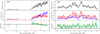 |
Fig. 3. XMM-Newton light curves of observations #74 (left) and #77 (right) with 100 s bin size. Each plot contains 3 panels: full light curve (top panel), soft (blue), and hard (red) light curves (middle panel) and hardness ratio (green; bottom panel). The data gaps correspond to GTI filters and high significance selection (data > error). |
Averaged count rates (in cps) of PN exposures on soft (0.5–6 keV) and hard (6–12 keV) energy bands and hard/soft ratio using 100 s bin light curves.
The top panel in the left plot of Fig. 3 shows the eclipse and the egress transition denoted by the two vertical dashed lines (time between ∼26 ks and ∼36 ks). The time interval of ∼10 ks of the eclipse egress we estimated from Fig. 3 corresponds to a phase interval of ∼0.025, which agrees with that of Coley et al. (2015) of 0.027 .
.
After the eclipse egress (#74c) the hard count rate stays almost constant around ∼0.5 cps, while the soft rate continues rising, leading to a hardness–ratio (HR) evolution. We performed a linear fit to the hardness ratio (log10HR = At + B) for the egress transition, obtaining A = −0.060 ± 0.003 cps ks−1 and B = 2.99 ± 0.14 cps ks−1 with a reduced χ2 = 0.84. Using this linear expression we estimated the time where HR < 1 (within errors), which resulted in ∼36 ks, with a corresponding phase in agreement with the egress-phase calculations (ϕe + Δϕe) of Coley et al. (2015).
In the right plot of Fig. 3, we present observation #77. During the entire exposure time, the hard emission dominates over the soft emission. The hardness ratio stays somewhat constant around ∼2. This behaviour is similar to that seen during the ingress of eclipse (#74b), where the hard emission dominated over the soft emission. In Table 2 we report the mean values and their standard deviations for every energy band and for all observations except for #74, as a linear fit was done. As can be seen from these values, for observations outside the eclipse, although hard emission is higher than that of the eclipse (#74 and #77), soft emission is much higher and dominates at every orbital phase.
In Table 2 we also included the absorption column density NH in units of 1022 cm−2. We find a positive correlation between the hardness ratio and the absorption column as expected. We note the latter is derived from spectral fitting and thus model dependent (see Sect. 3.2 for details), while light-curve colours are only sensitive to the response of the instruments.
Using 1 s bin light curves in the full energy range (0.5–12 keV) we performed spin-period searches using EFSEARCH task from HEASoft. This task returns a χ2 distribution of fitted periods in a given interval and resolution to the input light curve. We then proceeded to fit a Lorentzian profile to the maximum peak found to estimate the best-fit orbital-period and its uncertainty. According to Larsson (1996), the period error is overestimated by a factor of ∼20 with this method. Observation #74a (eclipse) was not included on the analysis. These results can be seen in Fig. 2.
A Doppler shift in the NS spin can be suggested before and after the eclipse (denoted by the dark grey vertical stripe in Fig. 2). Before the eclipse we register a weighted average of 140.015 ± 0.0008 s, which is higher than the corresponding 139.81 ± 0.02 s found after the eclipse (excluding observation #26, which corresponds to a different epoch). The NS spin is relatively larger (red–shifted) before the eclipse, when the NS is moving away from the observer, and shorter (blue–shifted) when it goes out of eclipse, moving towards the observer; thus the NS spin compatible with the expected Doppler shifts due to the short-period orbital motion of the NS around the high-mass stellar companion for a high–inclination system such as this eclipsing binary.
3.2. X-ray spectra
We extracted X-ray spectra in the same annular regions determined by the analysis of the EPATPLOT (see previous section) with an outer radius of 600 PhU. We used the same background regions indicated in the light-curve analysis. We generated redistribution response matrices (RMF) using RMFGEN, and ancillary response files (ARF) via ARFGEN tasks, respectively. Spectra were binned to 30 counts per bin with an over-sample factor of 3. We selected simple and double pattern events.
In general, the spectra of IGR J18027–2016 can be described well by an absorbed power-law-like continuum with high-energy cut-offs at energies above 7 keV. Features such as a soft excess at energies below 3 keV and Fe Kα (E ∼ 6.4 keV) and Fe Kβ (E ∼ 7 keV) emission lines and Fe absorption edge (E ∼ 7.2 keV) significantly vary among the whole data set.
Based on the light curve analysis and HR evolution found, for observation #74 we extracted three spectra, each corresponding to the eclipse (a), egress (b), and out-of-eclipse (c) periods described in Sect. 2.1. For each of the rest of the observations we extracted a single time-averaged spectrum, since no significant hardness-ratio variations were found. The eight resulting spectra along with the best-fit models and their residuals are shown in Fig. 4.
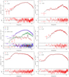 |
Fig. 4. The 6 spectra fitted in this work. We used a doubly absorbed NTHCOMP continuum model plus 2 Gaussian emission lines according to Table 4. Observation #74 was split onto 3 time periods: #74a (eclipse), #74b (egress), and #74c (out-of-eclipse). Orbital phases (ϕ) are indicated in each panel. |
We used a doubly absorbed thermally Comptonized continuum to model the spectra. One of the absorption components was used to take into account the extinction associated with the interstellar medium (ISM), while the second component, a partial-absorber model, was used to model intrinsic absorption and soft excess present during ingress towards eclipse observation #77.
In the language of XSPEC (Arnaud 1996), the model reads: TBABS*PCFABS*NTHCOMP. The ISM column density (TBABS model) was fixed to a value3 of NH = 0.8 × 1022 cm−2, while the covering fraction f (PCFABS model) was fixed to 1 in all observations except for obs #77 and #74b, which show a large excess at lower energies. The thermally Comptonized continuum model (NTHCOMP, Zdziarski et al. 1996; Życki et al. 1999) is parameterized by an asymptotic power-law index Γ, an electron temperature kTe, a seed photon energy kTbb, and an input type for black-body (inp_type = 0) or disc black-body (inp_type = 1) seed photons. In our case, we chose a scenario with black-body type seed photons. Both high– and low–energy rollovers were kept fixed to their default values of 100 keV and 0.1 keV, respectively, because they are outside the extracted PN spectrum energy range. Gaussian profiles were used to model the emission lines present on each spectrum.
We set the cosmic elements abundances to those of Anders & Grevesse (1989) and used photoelectric absorption cross-sections of Verner et al. (1996). To estimate continuum and line fluxes we used the CFLUX convolution model within XSPEC package. The total unabsorbed luminosity was calculated using a distance of 12.4 kpc. Errors in all parameters were calculated within the 90% uncertainty level using Markov chain Monte Carlo (CHAIN task in XSPEC). We set this up with the Goodman-Weare algorithm using eight walkers and 105 steps each.
In Fig. 4 we show the eight spectral fits with the bottom panel indicating χ2 deviations. Continuum parameters and fluxes are shown in Table 3 and the emission lines parameters and fluxes in Table 4.
Best-fit parameters for the continuum model of the extracted spectra.
Fe Kα and Fe Kβ detection probabilities (DP), line energies (E), widths (σ), and unabsorbed fluxes.
The Fe Kα (∼6.4 keV) and Fe Kβ (∼7 keV) emission lines were fitted for every observation, although the lines were not clearly resolvable in some of the observations. We tested for the presence of Fe Kα and Fe Kβ emission lines by running simulations using the FAKE-IT task from XSPEC. We fitted each line normalization (with fixed line energy and width), then drew 105 sampled spectra with the same model and continuum parameters, and proceeded to count how many of the sampled spectra had a line normalization greater than the normalization fitted to the real spectra. The ratio r between the latter number and the total sampled spectra gives an estimate of the probability of getting a normalization higher than the real spectra by chance. The smaller this ratio r, we can assume the actual presence of an emission line with greater confidence. We present these ratios as 1 − r in Table 4 in percentage units.
Line energies, widths, and fluxes were computed according to this table by establishing a lower tolerance of ∼99% (1 − r > 0.99). In some cases, line widths were left frozen or only computed an upper limit to fluxes. These are shown with a cross symbol in Table 4.
As can be seen from the obtained χ2 statistics, good overall fits were obtained from the NTHCOMP model. Pre-eclipse observation #77 had large soft excess at energies lower than 3 keV and thus was fitted with a free covering fraction. The covering fraction for this case gives 0.95 ± 0.01. The continuum shape remains very similar throughout the rest of the non-eclipsing observations (#75, #76 and #78), indicating that the NS accretion rate and wind density does not vary much along the orbit.
The spectral index becomes harder (≪1) for observations #77 and #74b, which also show an increase in the X-ray absorption, a decrease on X-ray fluxes, and a rising HR. Among all the out-of-eclipse observations, X-ray emission becomes softer and has indices closer to ∼1, which are typical values for these kinds of systems.
Outside the eclipse, IGR J18027–2016 unabsorbed luminosities oscillate between ∼1.0 L36, just exiting the eclipse, and ∼1.8 L36, according to its orbital phase (L36 = 1036 erg s−1). During the eclipse egress (#74b), the source luminosity increases by a factor of ∼50 with respect to the eclipse (#74a).
From the emission line perspective, observations #26 and #74c look featureless. Hill et al. (2005) carried out an F-test on observation #26 to check the presence of Fe Kα and could not confirm the line presence within 90% confidence region. According to Table 4, we can detect the Fe Kα line on observation #26 with a significance of ≲99%, while on observation #74c with a ≲46% significance. Thus, in both these cases we could give an upper limit to the line flux with its energy and width fixed.
Without emission lines, however these two observations present an absorption edge around ∼7.2 keV. To better describe this spectral feature we added an absorption EDGE convolution model to their respective continuum. The results were consistent within the two observations, giving a threshold energy of 7.15 keV and absorption depth of 0.23 ± 0.09.
Observations #77, #74a, and #74b present strong Fe emission lines and absorption edges. This effect comes from the fact that continuum emission is very diminished with respect to the other observations, also giving a higher equivalent width (EW). Observations #77 and #74b also present the highest measured values of absorption, of which the largest value was prior to the eclipse (see left panel of Fig. 5).
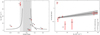 |
Fig. 5. Left: phase evolution of the absorption column density. The light grey stripes indicate ingress and egress transitions, while the dark grey stripe indicates the eclipse. The full black line corresponds to a Castor et al. (1975) wind model fit using system parameters from Coley et al. (2015). A clear excess over the model can be seen for phases previous to the eclipse, suggesting an additional contributing component than just wind absorption. Right: Fe Kα unabsorbed EW against the absorption column. The labels are phase ordered. The linear behaviour in non-eclipsing phases suggests that the Fe line emission region closely follows the NS orbital motion. |
To study the Fe Kα flux behaviour, along the orbit we computed its EW for each observation and compared it with the absorption column. The EW was calculated by computing the ratio of the unabsorbed Fe Kα flux to unabsorbed continuum flux, both between 6.1–6.7 keV. This plot is shown in the right panel of Fig. 5.
Outside the eclipse the EW seems to follow a positive linear correlation. We made a fit excluding low-significance data (Obs. #74 and #26), which resulted in a slope of 0.01 ± 0.003 with a reduced χ2 ∼ 0.54. This result agrees with that of Inoue (1985), which gave an approximate relationship between these two quantities:
 (1)
(1)
where N23 is the absorption column in units of 1023 cm−2. This expression corresponds to the case when the NS is totally hidden by a dense cocoon of matter and only scattered emission from the ambient matter is observed.
We also analysed the orbital evolution of the NS pulsed fraction (PF), shown in Fig. 6. The NS pulsed fraction was calculated by adopting the following definition:
 (2)
(2)
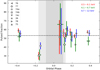 |
Fig. 6. Pulsed fraction (definition in text) for each observation calculated in 3 energy bands. Light curves used were folded with the best spin period found according to Fig. 2. The dashed horizontal line corresponds to the out-of-eclipse average value of 53 ± 5%. |
where Fmax and Fmin are the maximum and minimum values of the folded light curve (1 s bin on the given energy band) using the best period found for the respective observation according to Fig. 2. We calculated the PF for each observation on three different energy bands: 0.5–6.1 keV, 6.1–6.7 keV, and 6.7–12 keV.
We note that for every other non-eclipse observation the PF varies around an average value of 53 ± 5% (dashed horizontal line in Fig. 6) with a soft X-ray (< 6.1 keV) dominating component. But for the entering-eclipse observation #77, the total PF remains statistically below the averaged value and dominated by harder X-rays (> 6.7 keV).
4. Discussion
The classical picture of sgXBs involves a CO, typically a NS in a close orbit around a supergiant early star that has a strong wind embedding it and from which the CO is constantly accreting. By considering a simple spherical wind (Castor-Abbott-Klein (CAK), Castor et al. 1975), we can model the absorption orbital modulation by integrating the wind density profile along the line of sight for each orbital phase (see García et al. 2018, for a full description on this procedure). However, for a very low-eccentricity binary such as IGR J18027–2016, this method would produce a symmetrical absorption profile with respect to the eclipse mid-phase, which does not agree with the asymmetric absorption eclipse profile from IGR J18027–2016, as shown in Fig. 5. Since this asymmetry persists through several orbital revolutions, it is natural to invoke the presence of an asymmetric component, which could explain the increase of material between the observer and the NS when the latter is entering the eclipse and which has to be behind when the NS returns from the supergiant star at the eclipse egress.
A symmetric wind emanating from the supergiant companion cannot be the only explanation for the high absorption measured at the proximity of the eclipse (when the line of sight between the NS and the observer is almost tangent to the companion star), and the fact that outside the eclipse the absorption column is a factor of 3–10 times lower (remaining stable within errors). An over-density of absorbing matter, intersecting the line of sight towards the NS and enhancing the absorption column before the eclipse, is needed to explain both the asymmetry during the eclipse and the absorption columns measured in observations #77 and #74b. This asymmetry can be explained by considering a scenario in which a photo-ionisation wake is present (see Fig. 7). This density feature arises from the collision of the undisturbed radiation driven wind and the stagnant highly ionised plasma inside the NS Strömgren zone, producing strong shocks that create a dense sheet of gas that trails the NS. This kind of shock has also been proposed to explain asymmetric absorption profiles and the behaviour of hard X-ray light curves in other eclipsing HMXBs such as Vela X–1 and 4U 1700–37 (Kaper et al. 1994; Feldmeier et al. 1996; Malacaria et al. 2016).
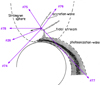 |
Fig. 7. Schematic representation of the model scenario. The photo-ionisation wake is responsible for the increased absorption column asymmetry before the eclipse. An accretion wake might also be present and increase absorption in phases previous to that of the eclipse. This figure is adapted from Kaper et al. (1994). |
Observational evidence for the presence of dense slabs of material in the accretion flow of IGR J18027–2016 are seen in the increase of X-ray hardness ratios towards eclipsing observations. Observations #77 (ingress) and #74b (egress) present an average hardness ratio 2–3 times higher than the observations far out-of-eclipse (see Table 2). The emitted soft X-rays are partly absorbed by regions of higher densities in the line of sight towards the CO at those orbital phases. The fact that the HR at the ingress to the eclipse is larger than that of the egress suggests that the photo–ionisation wake can account for this effect.
A couple of additional features are also expected owing to the presence of the NS within the stellar wind: First, an accretion wake trailing the NS, resulting from the accretion of perturbed wind by the passage of the highly supersonic NS; and second, a tidal stream, that is a stream of gas leaving the OB star and reaching the NS passing through the Lagrangian L1, formed by tidal interaction within the binary system. Both features are expected to be much less dense than the photo-ionisation wake, and thus contribute weakly to the obscuration of the CO (Blondin et al. 1990; Kaper et al. 2006; Malacaria et al. 2016). This accretion wake can account for the absorption, higher than the wind only, seen before the ingress to the eclipse (Obs. #76; see Fig. 5). The slightly increased hardness seen in this observation (see Table 2) can also contribute to this fact. More observations in between the phases −0.5 and −0.2 could help to determine the presence of an accretion wake more precisely. On the contrary, the tidal stream always being located in between the OB star and the NS, would not lead to an increased absorption. The lower pulse fraction seen in Fig. 6 indicates a deviation from spherical symmetry in the ingress to the eclipse. Furthermore, as the PF is statistically lower for energies < 6.7 keV, this suggests that this asymmetry affects lower energy photons preferably, and hence supporting the presence of the photo-ionisation wake.
These findings disagree with a discussion by Pradhan et al. (2019) in their recent paper on IGR J18027–2016 using the same XMM-Newton data set (however, we note our discussion about background and pile–up analysis in Sect. 2). The authors model the absorption by means of two variable models: one for Galactic absorption and another for the local absorption. With this method, they obtain much lower local absorption column densities than we do (with increased Galactic absorption instead). Although these authors obtain an increase of absorption before and after the eclipse, they argue that an accretion wake could not be formed on IGR J18027–2016 based on the premise that the stellar wind velocity of this system is large enough to not allow the formation of such structures.
The radius of influence of the X-ray pulsar is governed by its accretion radius and by the Strömgren sphere. It is expected that X-ray continuum emission should originate very close to the NS, generated by accretion of matter from the wind within these regions (Kaper et al. 1994). By means of the ionization parameter ξ we can estimate the size of this X-ray emitting region. This parameter is defined as ξ = LX/(n * R2), where LX is the illuminating X–ray luminosity, n is the surrounding gas density, and R its distance to the X-ray source. Furthermore, the matter density can be related to the absorption column density NH by NH = n * R. According to Inoue (1985), Fe ions up to Fe XIX can contribute to the bulge of the 6.4 keV Fe line profile. This ionization degree can be reached by ranges of ξ between 10 and 300.
We can estimate the size R of the emitting region, by taking into account the egress time interval (∼10 ks) when the X-ray luminosity increases by a factor of 50 (see Table 3), and using the NS orbital velocity. For the latter we used the same orbital parameters as for the NH model shown in Fig. 5. Thus, we obtain a region radius of ∼1.9 × 1012 cm or equivalently, ∼27 R⊙. If we now take into account the obtained luminosities and absorption columns from the spectral fits, we can give a range for the emitting-region size and density. Averaging LX and NH for non-near eclipse observations, we get a region size between 1011 cm and 3 × 1012 cm, or equivalently, between ∼1.4 and ∼43 R⊙. Furthermore, this region has a matter density ranging between 1.5 × 1010 cm−3 and 4.4 × 1011 cm−3.
The fact that our first R estimation lies very close to the higher end of the second estimation, suggests more firmly that Fe ions up to XIX might be present in the NS surroundings and contributing to the Fe Kα line complex. The positive linear correlation found between the unabsorbed Fe Kα EW and the absorption column density (Fig. 5), as well as the low pulsed fraction seen in Fig. 6, suggest that the Fe Kα line is generated close to the NS and that this accreted matter is also responsible for the absorption.
As we noted before, the Fe Kα line is generated in the vicinity of the NS. But the presence of the line during the eclipse indicates that these photons must come from another source, likely from reprocessing of X-ray photons by stellar wind particles, as already stated by Aftab et al. (2019). This effect has also been seen in eclipsing binaries such as Vela X–1, where the line EW during the eclipse is greater than 1 (as seen in Fig. 5).
5. Conclusions
In this work we have analysed six archival XMM-Newton observations of the eclipsing HMXB IGR J18027–2016 in addition to the 14-year cumulative, hard X-ray Swift/BAT light curve. Swift/BAT folded light curve shows that this source has an asymmetric eclipse profile that spans a fraction of ∼0.2 of the total orbital cycle (Porb ∼ 4.57 d).
XMM-Newton light curves in the soft (0.5–6 keV) and hard (6–12 keV) energy bands show similar flaring behaviour that is compatible with NS stellar wind accretion as the origin of the X-ray emission. Observations #74 and #77 show a very low soft rate (higher HR) compared to other observations, as a consequence of the high obscuration occurring during eclipse ingress/egress.
XMM-Newton time-averaged spectra show a highly absorbed power-law-like continuum with Fe line and absorption features (Fe Kα, Fe Kβ, and Fe absorption edge) strongly dependent on the orbital phase. Observations outside the eclipse show an absorption column density that is only lower than 10 × 1022 cm−2 and Fe Kα emission line. Eclipsing observations show a higher absorption column (NH > 30 × 1022 cm−2) and very strong Fe emission and absorption features. In particular, the absorption column before eclipse is ∼1.5 higher than that of the eclipse egress transition.
The NS PF remains close to 50% for all the observations except for that of the ingress #77. For the latter it must be that the emitting matter does not co-rotate as much as the other observations with the NS spin. Moreover, photons with energies < 6.7 keV are more heavily affected than those with greater energy, suggesting that this less co-rotating matter is located on the line of sight, thus absorbing and scattering low-energy photons.
The Fe Kα EW outside the eclipse follows a positive linear relationship with the absorption column. This indicates that the illuminated matter, where the Fe line originates, closely surrounds the NS, which is also responsible for the absorption of the X-ray photons. The presence of the Fe line during the eclipse (EW > 1) indicates that in this particular geometrical alignment, the emission line must be produced farther from the eclipsed NS because it is likely to be formed in the stellar wind that surrounds the companion star.
Finally, explain the asymmetric eclipse profile seen on the Swift/BAT hard X-ray light curve (Fig. 2), the absorption density column and hardness ratio orbital modulation (Fig. 5 and Table 2), we consider a photo-ionisation wake trailing the NS, where matter is concentrated between the NS and the companion star. Accretion wake presence is also suggested by an increased absorption during pre-eclipse phases.
More observations of this source, specifically at phases before the eclipse and after inferior conjunction (ϕ < 0) would be useful to better determine the presence and size of these large-scale wind structures. Joint analysis with detailed numerical simulations (see e.g., El Mellah et al. 2020) could provide great insight into the current picture of highly absorbed eclipsing sgHMXBs.
LAB weighted average obtained using the NH tool from the FTOOLs package.
Acknowledgments
F.A.F., F.G. and J.A.C. acknowledge support by PIP 0102 (CONICET). F.A.F. is fellow of CONICET. J.A.C. is CONICET researcher. This work received financial support from PICT-2017-2865 (ANPCyT). F.G. and S.C. were partly supported by the LabEx UnivEarthS, Interface project I10, “From evolution of binaries to merging of compact objects”. F.G. acknowledges the research programme Athena with project number 184.034.002, which is (partly) financed by the Dutch Research Council (NWO). This work was partly supported by the Centre National d’Etudes Spatiales (CNES), and based on observations obtained with MINE: the Multi-wavelength INTEGRAL NEtwork. JAC was also supported by grant PID2019-105510GB-C32/AEI/10.13039/501100011033 from the Agencia Estatal de Investigación of the Spanish Ministerio de Ciencia, Innovación y Universidades, and by Consejería de Economía, Innovación, Ciencia y Empleo of Junta de Andalucía as research group FQM-322, as well as FEDER funds.
References
- Aftab, N., Paul, B., & Kretschmar, P. 2019, ApJS, 243, 29 [NASA ADS] [CrossRef] [Google Scholar]
- Anders, E., & Grevesse, N. 1989, Geochim. Cosmochim. Acta, 53, 197 [Google Scholar]
- Arnaud, K. A. 1996, in Astronomical Data Analysis Software and Systems V, ASP Conf. Ser., 101, 17 [Google Scholar]
- Augello, G., Iaria, R., Robba, N. R., et al. 2003, ApJ, 596, L63 [NASA ADS] [CrossRef] [Google Scholar]
- Blondin, J. M., Kallman, T. R., Fryxell, B. A., et al. 1990, ApJ, 356, 591 [NASA ADS] [CrossRef] [Google Scholar]
- Castor, J. I., Abbott, D. C., & Klein, R. I. 1975, ApJ, 195, 157 [NASA ADS] [CrossRef] [Google Scholar]
- Chaty, S. 2013, Adv. Space Res., 52, 2132 [NASA ADS] [CrossRef] [Google Scholar]
- Chaty, S., Rahoui, F., Foellmi, C., et al. 2008, A&A, 484, 783 [NASA ADS] [CrossRef] [EDP Sciences] [Google Scholar]
- Coley, J. B., Corbet, R. H. D., & Krimm, H. A. 2015, ApJ, 808, 140 [NASA ADS] [CrossRef] [Google Scholar]
- El Mellah, I., Grinberg, V., Sundqvist, J. O., et al. 2020, A&A, 643, A9 [NASA ADS] [CrossRef] [EDP Sciences] [Google Scholar]
- Falanga, M., Bozzo, E., Lutovinov, A., et al. 2015, A&A, 577, A130 [NASA ADS] [CrossRef] [EDP Sciences] [Google Scholar]
- Feldmeier, A., Anzer, U., Boerner, G., et al. 1996, A&A, 311, 793 [Google Scholar]
- García, F., Fogantini, F. A., Chaty, S., et al. 2018, A&A, 618, A61 [CrossRef] [EDP Sciences] [Google Scholar]
- Hill, A. B., Walter, R., Knigge, C., et al. 2005, A&A, 439, 255 [NASA ADS] [CrossRef] [EDP Sciences] [Google Scholar]
- Inoue, H. 1985, Space Sci. Rev., 40, 317 [NASA ADS] [CrossRef] [Google Scholar]
- Kaper, L., Hammerschlag-Hensberge, G., & Zuiderwijk, E. J. 1994, A&A, 289, 846 [NASA ADS] [Google Scholar]
- Kaper, L., van der Meer, A., & Najarro, F. 2006, A&A, 457, 595 [NASA ADS] [CrossRef] [EDP Sciences] [Google Scholar]
- Krimm, H. A., Holland, S. T., Corbet, R. H. D., et al. 2013, ApJS, 209, 14 [NASA ADS] [CrossRef] [Google Scholar]
- Larsson, S. 1996, A&AS, 117, 197 [NASA ADS] [CrossRef] [EDP Sciences] [Google Scholar]
- Lebrun, F., Leray, J. P., Lavocat, P., et al. 2003, A&A, 411, L141 [NASA ADS] [CrossRef] [EDP Sciences] [Google Scholar]
- Liu, Q. Z., van Paradijs, J., & van den Heuvel, E. P. J. 2000, A&AS, 147, 25 [NASA ADS] [CrossRef] [EDP Sciences] [Google Scholar]
- Lutovinov, A., Rodriguez, J., Revnivtsev, M., & Shtykovskiy, P. 2005, A&A, 433, L41 [NASA ADS] [CrossRef] [EDP Sciences] [Google Scholar]
- Malacaria, C., Mihara, T., Santangelo, A., et al. 2016, A&A, 588, A100 [NASA ADS] [CrossRef] [EDP Sciences] [Google Scholar]
- Masetti, N., Mason, E., Morelli, L., et al. 2008, A&A, 482, 113 [NASA ADS] [CrossRef] [EDP Sciences] [Google Scholar]
- Negueruela, I., & Coe, M. J. 2002, A&A, 385, 517 [NASA ADS] [CrossRef] [EDP Sciences] [Google Scholar]
- Negueruela, I., Smith, D. M., Reig, P., Chaty, S., & Torrejón, J. M. 2006, The X-ray Universe 2005, 604, 165 [Google Scholar]
- Pradhan, P., Bozzo, E., Paul, B., et al. 2019, ApJ, 883, 116 [CrossRef] [Google Scholar]
- Sguera, V., Bazzano, A., Bird, A. J., et al. 2006, ApJ, 646, 452 [NASA ADS] [CrossRef] [Google Scholar]
- Strüder, L., Briel, U., Dennerl, K., et al. 2001, A&A, 365, L18 [NASA ADS] [CrossRef] [EDP Sciences] [Google Scholar]
- Torrejón, J. M., Negueruela, I., Smith, D. M., et al. 2010, A&A, 510, A61 [NASA ADS] [CrossRef] [EDP Sciences] [Google Scholar]
- Turner, M. J. L., Abbey, A., Arnaud, M., et al. 2001, A&A, 365, L27 [NASA ADS] [CrossRef] [EDP Sciences] [Google Scholar]
- Ubertini, P., Lebrun, F., Di Cocco, G., et al. 2003, A&A, 411, L131 [NASA ADS] [CrossRef] [EDP Sciences] [Google Scholar]
- Verner, D. A., Ferland, G. J., Korista, K. T., et al. 1996, ApJ, 465, 487 [NASA ADS] [CrossRef] [Google Scholar]
- Walter, R., Zurita Heras, J., Bassani, L., et al. 2006, A&A, 453, 133 [NASA ADS] [CrossRef] [EDP Sciences] [Google Scholar]
- Winkler, C., Gehrels, N., Schönfelder, V., et al. 2003, A&A, 411, L349 [NASA ADS] [CrossRef] [EDP Sciences] [Google Scholar]
- Zdziarski, A. A., Johnson, W. N., & Magdziarz, P. 1996, MNRAS, 283, 193 [NASA ADS] [CrossRef] [Google Scholar]
- Życki, P. T., Done, C., & Smith, D. A. 1999, MNRAS, 309, 561 [NASA ADS] [CrossRef] [Google Scholar]
Appendix A: XMM-Newton PN background treatment
In this section we describe the complete background treatment applied to the PN data set. This full description is important in this context to avoid introducing systematic errors on the light curves and spectra.
In Fig. A.1 we show the entire collection of background light curves. These were extracted using only high-energy (E > 10 keV) single events (PATTERN==0). We also excluded a circular region of radius 1200 PhU, surrounding the source IGR J18027–2016. The standard count-rate limit of 0.4 cps of the PN camera is indicated in each panel with a horizontal red line. As already described on Sect. 2.1, eclipse observation #74 presents a very high background activity but is not the only observation to do so. Obs #26, #75, and #78 also present flaring periods of several kiloseconds. In contrast, Pradhan et al. (2019) only report Obs #26 presenting flaring activity.
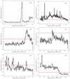 |
Fig. A.1. XMM-Newton PN high-energy (E > 10 keV) single events (PATTERN==0) background (excluding an enlarged source region) light curves with a 200 s bin size. Standard 0.4 count rate limit is indicated with the horizontal red line. |
To show these differences more clearly, we extracted images of the whole CCD with the same configuration of background light curves, but for high- and low-activity periods separately. In Fig. A.2 we show an example for observation #78. The left panel corresponds to the first 10 ks of the observation, where the average rate is ∼1.1 cps; the right panel represents the last 5 ks, where the average rate decreaces to ∼0.2 cps. Comparing both panels, it can be seen that these high-activity background periods illuminate the entire CCD, so no background region selected is free from contamination. Thus, if not removed accordingly, all further spectra and light curves are systematically hardened.
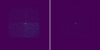 |
Fig. A.2. XMM-Newton PN high-energy (E > 10 keV) single events (PATTERN==0) images of observation #78. The left panel corresponds to first 10 ks of the background light curve (⟨rate⟩ ∼ 1.1 cps). The right panel the corresponds to the remaining exposure starting at 12 ks (⟨rate⟩ ∼ 0.2 cps). |
All Tables
Averaged count rates (in cps) of PN exposures on soft (0.5–6 keV) and hard (6–12 keV) energy bands and hard/soft ratio using 100 s bin light curves.
Fe Kα and Fe Kβ detection probabilities (DP), line energies (E), widths (σ), and unabsorbed fluxes.
All Figures
|
Fig. 1. Source and background light curves of the eclipse observation #74 using 100 s bins. Top panel: source+background (black) and background (red) light curves extracted in the 0.5–12 keV energy range using circular regions with equal area. Bottom panel: full CCD light curve in the 10–12 keV energy range excluding the source region. The black vertical lines indicate split times for eclipse (a), egress (b), and out-of-eclipse (c) periods, according to (Coley et al. 2015) ephemeris. The full (dashed) horizontal line corresponds to the background rate of 1 cps (0.4 cps). |
| In the text | |
|
Fig. 2. Top: folded Swift/BAT daily light curve using 32 phase bins with a period of 4.56993 d and mid-eclipse reference time of 55083.82 BMJD (Coley et al. 2015). The vertical light red stripes correspond to the six XMM-Newton observations used in this paper with their widths representing their final exposure times after GTI filtering. Bottom: neutron star spin periods for each observation, estimated by fitting a Lorentzian profile to the χ2 distribution of the period search. Observation #74a (eclipse) was not included in the analysis. Average spin periods of 140.015 ± 0.0008 s and 139.81 ± 0.02 s before and after the eclipse, respectively, are registered (excluding Obs #26, as it corresponds to a different epoch). Averages are indicated with dashed lines. |
| In the text | |
|
Fig. 3. XMM-Newton light curves of observations #74 (left) and #77 (right) with 100 s bin size. Each plot contains 3 panels: full light curve (top panel), soft (blue), and hard (red) light curves (middle panel) and hardness ratio (green; bottom panel). The data gaps correspond to GTI filters and high significance selection (data > error). |
| In the text | |
|
Fig. 4. The 6 spectra fitted in this work. We used a doubly absorbed NTHCOMP continuum model plus 2 Gaussian emission lines according to Table 4. Observation #74 was split onto 3 time periods: #74a (eclipse), #74b (egress), and #74c (out-of-eclipse). Orbital phases (ϕ) are indicated in each panel. |
| In the text | |
|
Fig. 5. Left: phase evolution of the absorption column density. The light grey stripes indicate ingress and egress transitions, while the dark grey stripe indicates the eclipse. The full black line corresponds to a Castor et al. (1975) wind model fit using system parameters from Coley et al. (2015). A clear excess over the model can be seen for phases previous to the eclipse, suggesting an additional contributing component than just wind absorption. Right: Fe Kα unabsorbed EW against the absorption column. The labels are phase ordered. The linear behaviour in non-eclipsing phases suggests that the Fe line emission region closely follows the NS orbital motion. |
| In the text | |
|
Fig. 6. Pulsed fraction (definition in text) for each observation calculated in 3 energy bands. Light curves used were folded with the best spin period found according to Fig. 2. The dashed horizontal line corresponds to the out-of-eclipse average value of 53 ± 5%. |
| In the text | |
|
Fig. 7. Schematic representation of the model scenario. The photo-ionisation wake is responsible for the increased absorption column asymmetry before the eclipse. An accretion wake might also be present and increase absorption in phases previous to that of the eclipse. This figure is adapted from Kaper et al. (1994). |
| In the text | |
|
Fig. A.1. XMM-Newton PN high-energy (E > 10 keV) single events (PATTERN==0) background (excluding an enlarged source region) light curves with a 200 s bin size. Standard 0.4 count rate limit is indicated with the horizontal red line. |
| In the text | |
|
Fig. A.2. XMM-Newton PN high-energy (E > 10 keV) single events (PATTERN==0) images of observation #78. The left panel corresponds to first 10 ks of the background light curve (⟨rate⟩ ∼ 1.1 cps). The right panel the corresponds to the remaining exposure starting at 12 ks (⟨rate⟩ ∼ 0.2 cps). |
| In the text | |
Current usage metrics show cumulative count of Article Views (full-text article views including HTML views, PDF and ePub downloads, according to the available data) and Abstracts Views on Vision4Press platform.
Data correspond to usage on the plateform after 2015. The current usage metrics is available 48-96 hours after online publication and is updated daily on week days.
Initial download of the metrics may take a while.