| Issue |
A&A
Volume 646, February 2021
|
|
|---|---|---|
| Article Number | A159 | |
| Number of page(s) | 13 | |
| Section | Planets and planetary systems | |
| DOI | https://doi.org/10.1051/0004-6361/202039271 | |
| Published online | 19 February 2021 | |
The GAPS Programme at TNG
XXIX. No detection of reflected light from 51 Peg b using optical high-resolution spectroscopy★,★★
1
INAF – Osservatorio Astrofisico di Catania,
Via S.Sofia 78,
95123
Catania,
Italy
e-mail: This email address is being protected from spambots. You need JavaScript enabled to view it.
2
INAF – Osservatorio Astronomico di Brera,
Via E. Bianchi 46,
23807
Merate,
Italy
3
Dipartimento di Fisica e Astronomia Galileo Galilei, Università di Padova,
Vicolo dell’Osservatorio 3,
35122
Padova, Italy
4
INAF – Osservatorio Astronomico di Roma,
Via Frascati 33,
00040
Monte Porzio Catone (RM), Italy
5
INAF – Osservatorio Astrofisico di Torino,
Via Osservatorio 20,
10025
Pino Torinese, Italy
6
INAF – Osservatorio Astronomico di Padova,
Vicolo dell’Osservatorio 5,
35122
Padova,
Italy
7
INAF – Osservatorio Astronomico di Capodimonte,
Salita Moiariello 16,
80131
Napoli,
Italy
8
INAF – Osservatorio Astronomico di Trieste,
Via Tiepolo 11,
34143
Trieste,
Italy
9
Thüringer Landessternwarte Tautenburg,
Sternwarte 5,
07778
Tautenburg, Germany
10
Dipartimento di Fisica G. Occhialini, Università degli Studi di Milano-Bicocca,
Piazza della Scienza 3,
20126
Milano, Italy
11
INAF – Osservatorio Astronomico di Palermo,
Piazza del Parlamento, 1,
90134
Palermo, Italy
12
Department of Physics, University of Rome “Tor Vergata”,
Via della Ricerca Scientifica 1,
00133
Rome, Italy
13
Max Planck Institute for Astronomy,
Königstuhl 17,
69117
Heidelberg, Germany
14
Aix-Marseille Univ, CNRS, CNES, LAM,
Marseille,
France
15
INAF – Osservatorio Astrofisico di Arcetri,
Largo Enrico Fermi 5,
50125
Firenze,
Italy
16
Dip. di Fisica, Sapienza, Universitá di Roma, Piazzale Aldo Moro, 2,
00185
Roma, Italy
17
Astronomy Department and Van Vleck Observatory, Wesleyan University,
Middletown,
CT
06459, USA
18
Fundación Galileo Galilei – INAF,
Rambla José Ana Fernandez Pérez 7,
38712
Breña Baja,
TF,
Spain
19
INAF – Osservatorio Astronomico di Cagliari & REM,
Via della Scienza, 5,
09047
Selargius
CA, Italy
Received:
27
August
2020
Accepted:
17
December
2020
Abstract
Context. The analysis of exoplanetary atmospheres by means of high-resolution spectroscopy is an expanding research field which provides information on the chemical composition, thermal structure, atmospheric dynamics, and orbital velocity of exoplanets.
Aims. In this work, we aim to detect the light reflected by the exoplanet 51 Peg b by employing optical high-resolution spectroscopy.
Methods. To detect the light reflected by the planetary dayside, we used optical High Accuracy Radial velocity Planet Searcher and High Accuracy Radial velocity Planet Searcher for the Northern hemisphere spectra taken near the superior conjunction of the planet, when the flux contrast between the planet and the star is maximum. To search for the weak planetary signal, we cross-correlated the observed spectra with a high signal-to-noise ratio stellar spectrum.
Results. We homogeneously analyze the available datasets and derive a 10−5 upper limit on the planet-to-star flux contrast in the optical.
Conclusions. The upper limit on the planet-to-star flux contrast of 10−5 translates into a low albedo of the planetary atmosphere (Ag ≲ 0.05−0.15 for an assumed planetary radius in the range of 1.5−0.9 RJup, as estimated from the planet’s mass).
Key words: techniques: spectroscopic / planets and satellites: atmospheres / planets and satellites: detection / planets and satellites: gaseous planets / planets and satellites: individual: 51 Peg b
Full Table 2 is only available at the CDS via anonymous ftp to cdsarc.u-strasbg.fr (130.79.128.5) or via http://cdsarc.u-strasbg.fr/viz-bin/cat/J/A+A/646/A159
Based on observations made with the Italian Telescopio Nazionale Galileo (TNG) operated by the Fundación Galileo Galilei (FGG) of the Istituto Nazionale di Astrofisica (INAF) at the Observatorio del Roque de los Muchachos (La Palma, Canary Islands, Spain).
© ESO 2021
1 Introduction
The atmospheric characterization of known exoplanets has tremendously developed since the first detection of an exoplanet atmosphere (Charbonneau et al. 2002). Transiting exoplanets are the most favorable targets for atmospheric characterizations. During transit, the outer layers of the gaseous envelopes of the planet filter the background stellar light and imprint features due to diffuse scattering and line absorption. In this regard, spectroscopic and photometric observations have proven to be a powerful tool for the atmospheric study of these bodies, both from space (e.g., Vidal-Madjar et al. 2004; Sing et al. 2009; Sotzen et al. 2020; Garhart et al. 2020) and from the ground (e.g., Nascimbeni et al. 2015; Mancini et al. 2017; Vissapragada et al. 2020; Guilluy et al. 2020; Sicilia et al., in prep.). Moreover, with the improvement of the available instrumentation, it has been possible to detect and analyze the phase curves and secondary eclipses of exoplanets, leading to the characterization of the planetary dayside (Stevenson et al. 2014; Parmentier & Crossfield 2018; Kreidberg et al. 2018; Singh et al. 2020).
Despite the lack of information from transits and eclipses, additional investigations have also been directed to non-transiting exoplanets with particularly interesting properties. In this respect, near-infrared and optical spectroscopy have been successfully adopted: in particular, the former aims to investigate the emitted spectrum of the planetary dayside (Brogi et al. 2012; Birkby et al. 2017), while the latter allows for the examination of the stellar reflected spectrum (Martins et al. 2015). Both techniques constrain the chemical composition and thermal structure of the planetary atmosphere. Moreover, if phase-resolved high-resolution spectroscopy is available, then it is also possible to measure the planet’s orbital velocity. This information is particularly valuable as it allows for one to determine the inclination of the orbital plane and, as a consequence, the true mass of the non-transiting planet. Thanks to a technique developed for double-lined spectroscopic binaries (Hilditch 2001), it is indeed possible to break the degeneracy between the planetary mass and the inclination of the orbital plane.
51 Peg b (HD 217014 b) is the first exoplanet to have been discovered around a solar-type star using the radial velocity technique (Mayor & Queloz 1995). So far, the search for planetary transits has failed (Mayor et al. 1995; Walker et al. 2006), and photometric techniques cannot provide the orbital inclination nor, consequently, the mass of the planet. Hence, the investigation of the planetary spectrum, which is either reflected or emitted, has been motivated by two reasons: the characterization of the planetary atmosphere and the measurement of the inclination of its orbit. The first successful high-resolution near-infrared spectroscopic analysis of 51 Peg b has been reported by Brogi et al. (2013) and later corroborated by Birkby et al. (2017), while the optical spectrum has been detected and analyzed by Martins et al. (2015) and Borra & Deschatelets (2018). All of these works suggest an orbital inclination between 70° and 80° as well as a planetary mass of approximately half a Jovian mass.
Nonetheless, the detection of the optical spectrum is still debated. Such a detection would imply that 51 Peg b has an unusually high geometric albedo for the class of hot Jupiters (HJs), and this makes it stand out in the search for elusive correlations between atmospheric properties and stellar irradiation (Heng & Demory 2013). Moreover, the same optical spectra have been reanalyzed by Di Marcantonio et al. (2019), who do not reproduce the claimed signal, yet they caution that their method could not reach the accuracy level needed for the detection of the signal.
In this regard, we here reanalyze and extend the previous analysis of optical spectra using all the available data in the High Accuracy Radial velocity Planet Searcher (HARPS) and High Accuracy Radial velocity Planet Searcher for the Northern hemisphere (HARPS-N) archives. Firstly, in Sect. 2 we provide a detailed mathematical framework, while in Sect. 3 we describe the analyzed datasets. In Sect. 4 we refine the ephemeris of 51 Peg b using the full set of radial velocity data available in the literature, complemented with the newest measurements. With our refined orbital solution, we chase the phase-resolved planetary signal as discussed in Sect. 5. Finally, in Sect. 6 we draw our conclusions.
2 Theoretical background
The spectroscopic observation of a planet-host star returns a spectrum which is, in principle, the superposition of the stellar spectrum and the planetary spectrum, regardless of whether the latter is due to the reflected stellar light and/or planet thermal emission. In particular, for the case of 51 Peg b, we expect that the contrast between the reflected flux and the stellar flux is on the order of 10−5 –10−4 in the optical domain (see below). As for the thermal emission, we can assume a stellar effective temperature of 5790 K and a stellar radius of 1.20 R⊙ (Fuhrmann et al. 1997), while for the planet we can assume an approximate radius of 1 RJup (see Sect. 6) and a conservative dayside temperature of 2000 K (Brogi et al. 2013; Birkby et al. 2017). Under these hypotheses, integrating the black body intensities in the spectral range covered a typical echelle spectrograph (3000–7000 Å), the thermal emission is an order of magnitude fainter than the expected reflected spectrum.
To set up the theoretical background needed for the interpretation of our results, we followed Perryman (2018) and the references therein. As explained above, we also neglect the emission component of the planetary spectrum.
2.1 The planet spectrum
If we define the planetary-to-stellar flux contrast at the orbital phase ϕ as ɛ(ϕ), then the spectrum reflected by the planet is given by:
 (1)
(1)
where vp is the phase-dependent radial velocity of the planet in the stellar rest frame, c is the speed of light in vacuum, and F*(λ) is the stellar spectrum in the stellar rest frame. If, for the sake of simplicity, we assume that the flux contrast ɛ does not depend on λ, and that the star slowly rotates in the planet’s rest frame, then the planetary spectrum is basically a rescaled version of the stellar spectrum that is Doppler-shifted by the radial velocity of the planet vp in the stellar rest frame.
Assuming that the planet is in a circular orbit, which is a reasonable approximation for 51 Peg b (as we derive in Sect. 4), then we can write
 (2)
(2)
where Kp is the radial velocity amplitude of the planet referred to the stellar rest frame, while ϕ is the orbital phase ranging in the 0–1 interval (ϕ = 0 corresponds to the planetary inferior conjunction).
As for the contrast ɛ in Eq. (1), we first define the phase angle α as the star-planet-observer angle given by:
 (3)
(3)
where i is the orbital inclination. The phase angle α determines the phase function g(α), which models the amount of the light reflected toward the observer. In an edge-on orbit (i = 90°), the phase function is 0 during a transit (when only the nightside of the planet is visible) and increases to 1 during a secondary eclipse, that is to say we would see the full dayside of the planet if it were not occulted by its host star. For the sake of simplicity, we assume that the planet follows Lambert’s scattering law, in which case the phase function is obtained analytically and is given by:
 (4)
(4)
The star–planet contrast thus depends on the orbital phase of the planet through the phase angle α as:
![Mathematical equation: \begin{equation*} \epsilon(\alpha)=\epsilon_{\textrm{max}}g(\alpha),~\textrm{with}~\epsilon_{\textrm{max}}=A_{\textrm{g}}\left[\frac{R_{\textrm{p}}}{a}\right]^2,\end{equation*}](/articles/aa/full_html/2021/02/aa39271-20/aa39271-20-eq5.png) (5)
(5)
where Ag is the geometric albedo of the planet and ![Mathematical equation: $[R_{\textrm{p}}/a]^2$](/articles/aa/full_html/2021/02/aa39271-20/aa39271-20-eq6.png) is a scaling geometrical factor, which sets the amount of stellar flux incident on the planet, and it depends on the planetary radius Rp and the orbital semi-major axis a. The phase function g(α) modulates the maximum planet-to-star flux contrast ɛmax along the orbital motion and defines the scattering properties of the atmosphere.
is a scaling geometrical factor, which sets the amount of stellar flux incident on the planet, and it depends on the planetary radius Rp and the orbital semi-major axis a. The phase function g(α) modulates the maximum planet-to-star flux contrast ɛmax along the orbital motion and defines the scattering properties of the atmosphere.
2.2 Properties of the cross-correlation function
Charbonneau et al. (1999) and Collier Cameron et al. (1999) estimated that, even in the most favorable cases of HJs, the flux contrast in the optical domain is lower than 10−4. This was later confirmed by Cowan & Agol (2011), who show that the albedo of HJs ranges between 0.05 and 0.4. For example, it would take a planetary radius of Rp = 1.7 RJ and a favorable albedo of Ag = 0.40 to make 51 Peg b shine 10−4 times as bright as its parent star. Because these are very optimistic conditions, this means that the planetary imprint in the stellar spectrum is most likely buried inside the noise of the spectra, and it is thus out of reach even for the best current spectroscopic facilities.
The cross-correlation function (CCF) technique has proved to be a powerful tool to boost the planetary signal and make it larger than the spectral noise (e.g., Snellen et al. 2010; Brogi et al. 2012). It essentially looks for the best match between an observed spectrum and a conveniently Doppler-shifted reference template, whether it be a binary mask or a model spectrum. In other words, the CCF is essentially the convolution of the observed spectrum and the template in the radial-velocity space. The result of the convolution, called CCF itself, is a good approximation of the average line profile and its signal-to-noise ratio (S/N) is approximately equal to the spectral S/N multiplied by the square root of the number of absorption lines in the reference template. The spectra analyzed in this work have S/N ~ 200 (Table 1), thus the S/N of the CCF would increase to 14 000 if the template contains 5000 lines, which is typical for binary masks used to process HARPS spectra. If we also consider that during each night of observations there are at least 40 spectra, the S/N of the cumulated signal would be ≳90 000, making it possible to detect a planetary signal as weak as 3 × 10⁻⁵ with a 3σ significance.
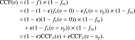
The aim of the CCF technique is to compute the average spectral line profile, while no emphasis is put on the spectral continuum. For this reason, the observed spectra are usually normalized to continuum, a procedure which does not affect the shape of the spectral lines. The normalization aims to avoid any bias introduced by the shape of the continuum, thus making it possible to compare spectra taken at different epochs with different airmasses and/or weather conditions. Hereon, we implicitly assume that the observed spectra and the model spectrum are normalized to continuum. Moreover, in the following, we do not cross-correlate the individual normalized spectra f and the corresponding model spectrum fm, but the functions 1 − f and 1 − fm. In this way, the continua of the observed and model spectra are set to zero and the absorption lines are turned upside down. The final effect is that the computation of the integral near the absorption lines provide a positive quantity, while it provides a null contribution elsewhere.
Borra & Deschatelets (2018) show the technical advantages of computing the CCF using a stellar template derived by averaging the observed spectra1. One of the most important things to specify is that the use of a binary mask may lead to mismatches in the positions and/or depths of the spectral lines, leading to the amplification of the noise in the CCF, while the average spectrum ensures a better match between spectra and templates. Secondly, the computation is less sensitive to numerical inaccuracies in the interpolation and integration processes. It is noteworthy that if a planetary signal is present, it shows up in correspondence of the radial velocity of the planet in the stellar rest frame straightaway, and no correction with respect to the stellar radial velocity is needed. For these reasons we follow the approach of Borra & Deschatelets (2018), that is to say the computation of the CCF using an average stellar spectrum to homogeneously analyze the sets of spectra listed in Table 1.
From a theoretical point of view, if we convolve a spectrum with Gaussian-shaped lines, all with the same variance  , with a model spectrum whose lines have a width of
  , then the CCF is a Gaussian function with variance given by
  . In particular, if the spectrum and the model are characterized by the same σo, then the variance of the CCF is simply
  . We can thus model the CCFo of a stellar spectrum f*(v = 0) in its rest frame and the model spectrum fm as:
 (6)
(6)
where A is the amplitude of the Gaussian function and δ is an offset term. The latter is due to the fact that there is some random overlap among the lines pattern in the observed and model spectra, respectively, even when the two are not aligned. This means that even in the case of misalignment, the convolution does not return a null result. This offset δ is, in principle, a function of v as it depends on how the line pattern in the observed and model spectra cross-correlate in the velocity space. As we will show in Sect. 5.2, departures from a constant value show up as correlated noise in the CCF continuum, whose degree of correlation depends on the line broadening in the model and observed spectra.
Log of the observations analyzed in this work.
2.3 The planet CCF
We now assume that the observed spectrum F in the stellar rest frame is the combination of the stellar spectrum F* and the spectrum reflected by the planet Fp as in Eq. (1):
 (7)
(7)
The stellar spectrum can be factorized into the continuum spectrum Fc and the line spectrum f*, where the latter equals 1 where there is no line absorption and decreases toward zero according to the opacity profile of the absorption lines. The f* factor thus corresponds to the normalized spectrum introduced in the previous section:
 (8)
(8)
where we have made the dependency on the velocity v of the source explicit. Since both Fc and f* depend on v, then the planetary spectrum Fp, in principle, shifts with respect to the stellar spectrum both in terms of the continuum spectrum and line spectrum.
In the general case of a planet orbiting its host star, the rotational velocity is such that the maximum Doppler shift in the optical domain corresponds to a few Å. In the specific case of 51 Peg b, assuming the orbital speed of 132 km s−1 (Brogi et al. 2013; Martins et al. 2015; Birkby et al. 2017; Borra & Deschatelets 2018), the maximum Doppler shift at 5000 Å is 2.2 Å. We assume that this shift is not large enough to introduce a significant displacement to the continuum spectrum. In other words, we can reduce the dependency of Fc on v. Inserting Eq. (8) in Eq. (7), we thus derive:
 (9)
(9)
The last term in Eq. (9)
 (10)
(10)
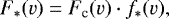
has the physical meaning of a normalized spectrum, as it is equal to 1 for the wavelengths not affected by line absorption, and it decreases toward zero in correspondence of the spectral lines in the stellar and planetary spectra (f* (v = 0) and f* (v = vp), respectively). In this regard, the term (1 + ɛ)Fc in Eq. (9) corresponds to the continuum spectrum.
The expected contrast ɛ is on the order of 10−4 or below. We can thus compute the Taylor expansion of Eq. (9) in powers of ɛ to derive:
 (11)
(11)
This equation shows that the observed normalized spectrum is the weighted average of the stellar and planetary normalized spectra. Moreover, in the case of vp≠0, that is to say when the stellar and reflected spectra are not aligned, the intensity of the absorption lines in the observed spectrum is lower than the purely stellar one, as the presence of the planetary spectrum fills in, or veils, the line component of the stellar spectrum.
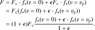
Convolving the spectrum in Eq. (11) with the stellar model, and using the linearity of the convolution operator, we derive:
 (12)
(12)
We hereby remark that the combined CCF is the weighted mean of the stellar and planetary CCFs.
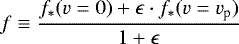
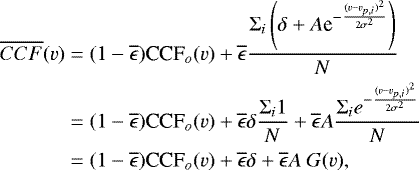
The goal of the method is to measure the amplitude of the planetary contribution ɛ in Eq. (12) in order to derive the albedo Ag from Eq. (5). Since we expect that the contrast ɛ is on the order of 10−4 or lower, then the expected amplitude of the planetary CCF is small and buried in the noise of the wings of the stellar CCF. This noise is difficult to quantify a priori, as it is a mixture of a random component due to the noise in the observed spectra and the correlated noise in the offset δ discussed above. This last term is usually the largest one at this stage. It shows the same pattern in the CCF of all the spectra and can be minimized by normalization with an average CCF profile. Again, by the linearity property, the average  can be written as:
![Mathematical equation: \begin{align*} \overline{CCF}(v)=&\,\frac{\Sigma_i \left[(1-\epsilon_i)\textrm{CCF}_o(v)+\epsilon_i \textrm{CCF}_o(v-v_{p,i})\right]}{N}\nonumber\\ \simeq&\,\frac{\Sigma_i(1-\epsilon_i)}{N}\textrm{CCF}_o(v)+\frac{\Sigma_i \overline{\epsilon}\textrm{CCF}_o(v_{p,i})}{N}\nonumber\\ =&\,(1-\overline{\epsilon})\textrm{CCF}_o(v)+\overline{\epsilon}\frac{\Sigma_i \textrm{CCF}_o(v_{p,i})}{N},\end{align*}](/articles/aa/full_html/2021/02/aa39271-20/aa39271-20-eq19.png) (13)
(13)
where we assume that the contrasts ɛi can be approximated by the average contrast  (this is the typical case of spectra taken within the same night of observations). Incidentally, we note that the last line in Eq. (13) corresponds to the CCF of the average spectra in Eq. (11).
Inserting Eq. (6) in the last term of Eq. (13), after simple math we derive:
 (14)
(14)
where we define
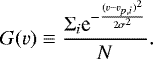 (15)
(15)
Equation (15) is the average of a set of shifted Gaussian functions and it represents the dilution of the planetary signal in the average CCF depending on the velocities vp,i spanned by the planet. If the velocities vp,i differ by many σ, then the exponential terms do not overlap, and the function G(v) is basically the series of N Gaussian functions, each one centered at its corresponding vp,i and whose amplitude is 1∕N. Conversely, for our typical datasets, the planetary CCFs drift by less than σ from one observation to the next, such that the exponential functions in Eq. (15) partially overlap. This means that the individual exponential contributions cannot be distinguished by the shape of the function G(v), which tends to be a value ≲1 when v runs in the velocity range encompassed by the set vp,i, and it tends to be 0 as v runs out of this range.
The average CCF in Eq. (14) can now be used to normalize the CCF of the individual spectra (Eq. (12)), obtaining:
 (16)
(16)
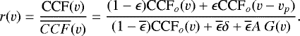
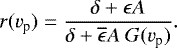
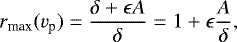
The r(v) thus represents the amplitude of any Doppler-shifted signal with respect to the continuum of the average CCF.
In Fig. 1 we plot Eq. (16) assuming Eq. (6) with σ = 10.6 km s−1, A = 3000, and δ = 1000, which are a good approximation for the width, amplitude, and continuum level of the CCF of our observed spectra, respectively. We also adopted the maximum contrast of ɛmax = 10−4 and the orbital inclination i = 80° (Borra & Deschatelets 2018), together with the orbital solution obtained in Sect. 4 to compute the phase-dependent planet-to-star flux ratio as in Eqs. (4)–(5). For G(v), we simulated 70 observations evenly spaced in time, ranging from phase ϕ =0.4 to ϕ =0.5. For simplicity, we discuss three different velocity domains directly below.
Firstly we discuss the case when the stellar model is far from matching both the stellar and the planetary spectrum (∣ v∣ > 4σ and ∣ v − vp∣ > 4σ). In this scenario all the exponential terms in Eq. (16) are negligible, and we obtain:
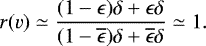 (17)
(17)
This result shows that the function r(v) is indeed the normalization of the CCF. We also remark that the normalization minimizes the effects of the correlated noise pattern in the offset δ.
The second domain we discuss is when the stellar model is close to matching the stellar spectrum and the planetary CCF is far enough in the velocity space so as to not contaminate the stellar CCF (∣ v∣ < 4σ and ∣ v − vp∣ > 4σ). With these assumptions the exponential terms due to the planetary CCFs in Eq. (16) are negligible. By consequence, if we approximate , then the numerator and the denominator are the same, and we can write r(v)≃ 1. This result formalizes the fact that we can erase the dominant stellar signal by division with
  .
.
The last domain is when the model matches the planetary CCF, the latter being well resolved from the stellar CCF (∣ v∣ > 4σ and ∣ v − vp∣ < 4σ). In this case, Eq. (16) can be approximated as:
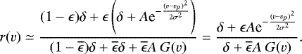 (18)
(18)
In particular, the amplitude of the planetary signal is obtained substituting v = vp:
 (19)
(19)
This result shows that the amplitude of the planetary signal is a function of the maximum contrast ɛ, the stellar CCF’s parameters A and δ, and the sampled planetary velocities vp,i through G(v). In the best-case scenario, the planetary signal in the average CCF is completely diluted such that G(vp) = 0 and, by consequence, the maximum signal we can extract is:
 (20)
(20)
that is to say the maximum planetary signal would have the amplitude ɛA∕δ over the continuum.
In a more realistic scenario, we cannot neglect the contribution of G(vp), which being a positive quantity reduces the signal r(vp). As a matter of fact, by making the approximation  and by means of Taylor expansion in powers of ɛ, we can rewrite Eq. (19) as:
 (21)
(21)
that is to say the contrast of the planetary signal against the continuum is reduced by a factor 1 − G(vp) with respect to rmax(vp). For the datasets we analyze in this work, following the definition in Eq. (15), we have G(vp) ≃ 10−2−10−1, that is to say the planetary signal is reduced by 10% at most.
From a different perspective, the effect of G(vp) in Fig. 5 is to lower the continuum of the r(v) function in the velocity range spanned by the planet, so as to decrease the strength of the planetary signal. Incidentally, we remark thatthis effect was ignored by Martins et al. (2013) and it may explain why they could not retrieve exactly the same signal that they injected in their simulations. Moreover, the decrease in the continuum level is present in the examples shown by Borra & Deschatelets (2018), but the authors do not discuss its origins and effects.
Equation (19) and Fig. 1 solidify the fact that the best orbital phases to sample to maximizethe amplitude of the planetary signal are those closest to superior conjunction. Most importantly, they show that when several spectra that are taken during the same night are averaged, the planetary signal in the average CCF is diluted over the orbital velocities. The direct effect is that if the observations cover a conveniently large range of orbital velocities, the amplitude of the planetary signal in the average CCF is greatly reduced, and the normalization does not cancel the individual planetary CCFs. Nonetheless, we find that for 0.48≲ ϕ ≲ 0.52, the planetary CCF becomes too close (less than 4σ) to the stellar counterpart, such that the approximations in Eq. (19) do not hold anymore. In particular, when the planetary and the stellar CCFs are less than ~4σ apart, that is to say when the planetary and stellar spectra blend in the wavelength space, they tend to mimic a purely stellar spectrum. The main effect is that the stellar and planetary CCFs cannot be resolved anymore. Substituting v = vp in Eq. (16), and by means of Eq. (6), we obtain:
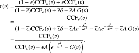 (22)
(22)
Due to the definition in Eq. (15), the bracketed quantity in Eq. (22) is always positive, and this explains the bump in Fig. 1 at phase ϕ = 0.5. We note that it is not easy to analyze this bump to extract the planetary CCF, both because of its mathematical formalization and the reduced amplitude compared with earlier (and later) orbital phases. We thus would relax the statement of Borra & Deschatelets (2018) according to which the planetary signal can also be extracted at a superior conjunction.
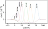 |
Fig. 1 Expected planetary signal as discussed in the text. Different orbital phases approaching superior conjunction are simulated, as annotated in the plot. The parameters adopted for the simulations are ɛmax = 10−4, σ = 10.6 km s−1, A = 3000, and δ = 1000 (Eq. (16)), together with the orbital solution derived in Sect. 4. |
3 Observations and data reduction
We observed the 51 Peg system as part of the GAPS program for the TNG (PI: G. Micela, Covino et al. 2013) in GIARPS mode (Claudi et al. 2017), which allows for simultaneous coverage of the optical and near-infrared spectral bands. In this work we only analyze the optical spectra provided by the HARPS-N instrument (Cosentino et al. 2012), a collection of two sets of observations for the nights of 26 and 27 July 2017, for a total of 159 spectra. The infrared spectra are currently under analysis and they will be discussed in a future publication. We complement our dataset with publicly available data, taken with the same purpose of measuring the light reflected by the HJ in the system. The full list of datasets is in Table 1.
The dataset of program 091.C-0271 has been analyzed by Martins et al. (2015), who claim a positive detection of the reflected light and quantify the flux ratio between the planet and the star on the order of 10−4. Their claim has also been confirmed by Borra & Deschatelets (2018) with an improved data analysis. Di Marcantonio et al. (2019) reanalyze the same data using the Independent Component Analysis (Hyvärinen 2001) and they attempt to recover the possible reflected spectrum of 51 Peg b which gave no conclusive results. The authors report that the usage of the ICA methodology to extract a reflected spectrum from the host star is a novel technique and simulations have shown that requirements on S/N are more stringent. Despite this, a low detection significance has been obtained even when a different estimator was compared with the work by Martins et al. (2015) and Borra & Deschatelets (2018), which led the authors to be cautious in claiming reflected light detection.
As we discuss in the following, our data analysis requires that many spectra be taken within the same night of observation. For this reason, we do not analyze the full library of spectra from the HARPS archive, as they were sparsely collected across different nights (see the itemized list above for the dates spanned by each program). We only selected the 39 (out of 91) spectra taken on the night of 2013 September 20 for program 091.C-0271 and the 48 (out of 218) spectra taken on the night of 2018 October 21 for program 101.C-0106. These two subsets are the largest collections of back-to-back spectra provided by the two programs. The remaining spectra were collected occasionally on different dates and we only use them for the refinement of the orbital solution (Sect. 4), not for the extraction of the reflected spectrum (Sect. 5). Moreover, we rejected the last 31 spectra from the night of 2016 November 02 (program CAT16B_43) as they were taken during bad weather conditions. All of the collected spectra were taken in proximity of the superior conjunction of the planet, so as to maximize the planetary phase function (Eq. (4)). The final number of analyzed spectra in each program is reported in Table 1.
Our approach for data reduction and analysis works separately for each night of observation. The following description of the workflow thus applies on a night-by-night basis. Only at the end did we merge the nightly results in order to boost the signal detection.
For each night of observation, we analyzed the s1d spectra provided by the DRS pipeline using the SLOPpy (Spectral Lines Of Planets with python) pipeline (Sicilia et al., in prep.). SLOPpy is a user-friendly, standard and reliable tool that is optimized for the spectral reduction and the extraction of transmission planetary spectra obtained from high-resolution observations. For this purpose, SLOPpy first applies several data reduction steps that are required to correct the input spectra for sky emission, atmospheric dispersion, and the presence of telluric features and interstellar lines. These last reduction steps were not performed by the DRS pipeline. Even though our aim is not the extraction of a transmission spectrum, we used the SLOPpy pipeline as its reduction steps are designed to preserve the planetary signal.
The telluric correction was performed inside SLOPpy using MOLECFIT (Smette et al. 2015; Kausch et al. 2015). In order to compute the best telluric model, we considered that those wavelength ranges were not contaminated by stellar lines to inject to MOLECFIT. We made the selection of wavelength ranges only once per night and we used it for all the spectra of the same night. This approach was motivated by the fact that during the night, the stellar and telluric spectra do not shift significantly with respect to each other, and blends involve the same group of lines along the series of spectra. By visually checking the result of the telluric removal, we find that no residuals are left above the noise level, with the exception of some leftovers that are comparable with spectral noise for the O2 lines at wavelengths longer than ~6250 Å (Fig. 2). In Sect. 5, we check that these systematic residuals do not hamper the CCF analysis.
We set up SLOPpy such that the reduced spectra were shifted in the stellar rest frame using the RV measured by the data reduction pipeline and interpolated over the same wavelength grid. Due to differential refraction, the average continuum level of the spectra can show a flux imbalance as a function of the airmass which, if not corrected, may affect the telluric correction and the whole analysis. The SLOPpy pipeline models this effect using a low-order polynomial or a spline, depending on the cases, and it recalibrates the spectra to the same continuum using this model. We used these recalibrated spectra to remove some spikes, which were likely due to cosmic rays hits. For each wavelength bin, we computed the median and the median absolute deviation (MAD) of the fluxes, we rejected all the pixel values which deviate more than 5 MAD from the median and substituted them with the median flux. This typically corrects only a few pixels, or small groups of pixels, per spectrum.
After the removal of spikes, we refined the alignment of the spectra. To do so, we selected the spectrum with the best S/N in the series and aligned all the remaining spectra by maximizing the cross-correlation with the selected high S/N spectrum. The most important aspect here is that the best alignment among the spectra is ensured, while the absolute radial velocity calibration, which is now the same for all the spectra, does not bias the search for the planetary signal, as shown in Sect. 2.
In Sect. 2 we also explain why it is convenient to work with normalized spectra. The steps we followed to accomplish spectral normalizations are the following. First of all, we masked out the wavelength ranges 4815–4845, 5130–5210, 5887.5–5897.5, and 6552.8–6572.8 Å, which contain the broad Hβ line, the Mg I triplet, the Na I doublet, and the Hα line, respectively. Then we divided the spectra into 50 bins with the same width, and for each bin we computed the median value after clipping the absorption lines. Finally we interpolated the 50 median values over the original wavelength grid using a spline function, thus obtaining the continuum spectrum used for normalization purposes.
We remark here that neither the spike removal nor the normalization are expected to interfere with the planetary signal if present. As a matter of fact, the former acts sparsely on a few pixels and only in some spectra of the series, while the latter operates on wavelength scales much wider than the full width at half maximum (FWHM) of the spectral lines.
Finally, once the data reduction was complete, we first computed the reference spectrum of each night of observation as the median-average of the series of spectra, and then computed the residuals of each observed spectrum with respect to the corresponding reference spectrum. This residual spectrum was thus processed through a moving average algorithm to extract the noise model. This procedure was done individually for each spectrum as the noise model may vary with time according to the airmass or changing weather conditions, for example. The noise model, of which there is one for each spectrum, is useful in Sect. 5 where we test our analysis algorithm. The noise model we computed is consistent with the noise estimated by the HARPS and HARPS-N data reduction pipelines, and it does not show the typical artifacts which occur when the spectra are not perfectly aligned with the template.
 |
Fig. 2 Example of the result of the telluric correction discussed in the text. |
RV measurements analyzed for the refinement of the orbital solution.
4 Orbital solution
To refine the ephemeris of 51 Peg b, we used the list of RV data already piled-up by Birkby et al. (2017), which consists of 639 measurements by several instruments (ELODIE, Lick, HIRES, HARPS) running from BJD = 2 449 611 (September 1994) to BJD = 2 456 847 (July 2014). The HARPS RV measurements in this collection correspond to the program 091.C-0271 analyzed in this work(see Table 1). Since we noticed slight differences in the times of observations and RV uncertainties with what is provided by the HARPS data reduction pipeline, for consistency, we updated the collection ofBirkby et al. (2017). Finally, we updated and extended the same collection with the more recent programs listed in Table 1. The final list contains 1260 RV measurements (Table 2).
We fit the RV measurements using the PyORBIT package2 (Malavolta et al. 2016), trying both the circular and the eccentric Keplerian models. The eccentric fit resulted in a negligible eccentricity (e = 0.007 ± 0.003) according to the Lucy & Sweeney criterion (Lucy & Sweeney 1971), which is consistent with previous analyses (e.g., Naef et al. 2004; Birkby et al. 2017). Moreover, we find no significant change in the other orbital parameters between the eccentric and circular fits. We thus report the results of the fit of the circular model.
The priors on the orbital period P and the RV semi-amplitude K were set to be uniform and centered on the estimates already available in the literature, but much larger than the corresponding uncertainties, resulting in uninformative priors (Table 3). For each instrument, we also fit an independent jitter term to account for different instrumental white noise levels and the underestimation of the uncertainties by the different reduction pipelines. An independent RV offset for each instrumental setup was also included. For the HARPS at ESO data, we set two independent offsets to account for the upgrade of the fiber and the possible offset drift (Lo Curto et al. 2015). We adopted a similar approach for the three data series from the Lick observatory, which were taken with different upgrades of the instrument.
Following Birkby et al. (2017, and the references therein), we also explored the possibility that the data contain evidence of a long-term trend, a controversial claim which has not been firmly confirmed or disproved yet. We find no evidence of such a trend, and since the orbital parameters do not change significantly if we add a linear term to the fit, in this paper we report the results assuming the simpler model with no long-term drift.
We let the Monte Carlo code run for 100 000 steps, which turns out to be as long as ~300 times the auto-correlation length of the chains, which were computed following Goodman & Weare (2010). This indicates that the fit has successfully converged, as suggested by Sokal (1997) and adapted to parallel Monte Carlo chains3. Moreover, the obtained posterior distributions look to be nicely centered on the maximum-a-posteriori (MAP) best-fitting values, reported in Table 3 together with the corresponding 16–84% quantiles. Our results are in general agreement within 2σ with the latest ephemeris published by Birkby et al. (2017). The best fit model and the residuals are shown in Fig. 3, while Fig. 4 shows the subset of RV measurements relative to the spectra used for the extraction of the planetary signal (Sect. 5).
The prior on stellar mass M* = 1.07 ± 0.03M⊙ used to compute the planetary mass was obtained using the PARAM web interface version 1.54 (da Silva et al. 2006; Rodrigues et al. 2014, 2017), with the spectroscopic parameters Teff= 5814 ± 19 K, [Fe/H] = 0.21 ± 0.01 dex, and log g = 4.35 ± 0.03 dex (Sousa et al. 2018) as listed in the SWEET-Cat catalog5 (Santos et al. 2013). The parallax  mas was taken from the Gaia DR2 (Gaia Collaboration 2018), while the near-infrared magnitudes were taken from the 2MASS catalog (Skrutskie et al. 2006). The stellar luminosity and the asteroseismic parameters were left undefined in PARAM, and default options were used for the computation. The uncertainty on the stellar mass takes into account the difference between the independent estimates provided by PARAM when using the two different sets of implemented evolutionary models (PARSEC Bressan et al. 2012 and MESA Rodrigues et al. 2017 isochrones).
Updated orbital solution for 51 Peg b.
5 Data analysis
To enhance the detectability of the stellar light reflected by 51 Peg b, we used the CCF technique described in Sect. 2. In the computation of the CCF, we did not use the full wavelength coverage of the spectra (~3800–6900 Å). As a matter of fact, we discarded the spectral range λ < 4500 Å because the bluest echelle orders are the noisiest ones and accurate continuum normalization cannot be achieved. We also discarded the range λ > 6700 Å as it is heavily contaminated by saturatedtelluric absorption by O2, which cannot be accurately corrected by MOLECFIT. Moreover, the HARPS spectra do not cover a wavelength window of ~100 Å around 5300 Å. To make the datasets comparable with each other, we cut the 5250–5350 Å wavelength range in all the spectra in Table 1, as it is the shortest cut which excludes the blind range in all HARPS spectra. Finally, in Sect. 2 we explain why the width of the CCF increases with the width of the line profile of the model spectrum. The model spectrum we used is the median-average of the observed spectra, which contain, among others, a variety of broad lines. This has two main effects which we want to avoid: the increase of both the width and the correlated noise of the CCF. For these reasons, we removed the spectral ranges containing all the lines that, after a by-eye inspection, clearly show broadened Lorentzian profiles. The wavelength ranges that are cut off the spectra are listed in Table 4.
5.1 Analysis of simulated datasets
Before analyzing the data, we ran a few simulations to test the robustness of the method. The first step was thus to simulate datasets where we injected a known signal. For this purpose, for each night of observations, we used the corresponding average spectrum asa model template and we generated the simulated spectra assuming the same orbital phases sampled during the night. We injected the planetary spectrum assuming the ephemeris in Sect. 4, together with Kp =132 km s−1, ɛmax = 10−4, and i = 80° (consistently with Borra & Deschatelets 2018) and by computing the planetary spectrum, velocities, and phase functions according toEqs. (1)–(5). To each simulated spectrum, we finally added random noise using the noise model we mention in Sect. 3. In Fig. 5, we plotted an example of the simulation, using the dataset from 2017 July 27 in Table 1: the individual CCF and the average  are identical within noise, such that the planetary signal cannot be discerned. Even after normalization, the noise in the r(v) function is on the order of a few 10−4, thus comparable with the injected signal. Hence, the analysis of the individual CCFs cannot lead to the detection of the expected signal.
To enhance our capability of detecting the planetary signal, we adopted the approach of Martins et al. (2015) and Borra & Deschatelets (2018). In principle, we do not know where the planetary CCF is located with respect to the stellar CCF, as we do not know in advance the value of Kp to insert in Eq. (2). We thus built a grid of tentative Kp values and, for each one, we computed the radial velocities corresponding to the phases sampled by the observations. For each tentative Kp value, we could thus recenter all the r(v) functions inthe corresponding planetary reference frame such that if the assumed Kp were correct, the planetary signals would thus be all centered at v = 0. The main assumption of this procedure is that the average amplitude  is maximum when the correct value of Kp is used to recenter the CCFs. Conversely, if the assumed Kp is wrong, then the planetary signals of the wrongly recentered r(v) functions do not match in the velocity space. In all of these cases,
  is expected to be distributed around 0 with a standard deviation approximately given by the noise of the original r(v) scaled down by a factor
  , where N is the number of spectra.
We further optimized this procedure by adopting two additional criteria. Firstly, we remarked that during each night of observation, the flux contrast changed according to the orbital phase (Eqs. (3)–(5)). With the aim of giving more emphasis to the observations closer to superior conjunction, we computed  weighting the set of r(v) functions by the corresponding g(α) (Eq. (4)). This procedure is particularly useful when we jointly analyze all the CCFs, whose phase function g(α) ranges from ~0.66 to ~0.98. We remark here that the phase function in Eq. (4) only applies to a Lambertian spherical surface, which may not be the case of 51 Peg b. However, in the general case of a back-scattering atmosphere, any alternative to Eq. (4) is a function which monotonically increases toward superior conjunction. Using different formulations of the phase function still puts more emphasis on the spectra taken closer to superior conjunction and introduces second order corrections to the final result. Secondly, we excluded all the spectra taken too close to superior conjunction. In regards to Fig. 1, we excluded the range 0.48 < ϕ < 0.52, because in this phase interval the planetary and stellar CCFs are blended and thus cannot be separated. This rejection criterion excludes 5, 43, and 40 spectra taken on 2015 October 27, 2016 October 12, and 2016 October 29, respectively (Table 1).
As an example, we applied this approach to the same simulated datasets discussed thus far (date 2017 July 27). Figure 6 clearly shows that the planetary signal peaks close to the assumed Kp = 132 km s−1. As expected, we also find that random noise in the continuum of  has scaled down approximately by the square root of the number of spectra. We further improved the detection of the planetary signal by extending our approach to the full dataset: After the exclusion of the 88 spectra close to superior conjunction, 411 spectra were left in total and random noise further decreased by a factor of ~2.
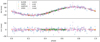 |
Fig. 3 Phase-folded diagram of the analyzed RV measurements using the ephemeris listed in Table 3 (top panel) and corresponding residuals (bottom panel). Measurements from different instruments are marked with different symbols as shown in the legend. The “Lick6,” “Lick8,” and “Lick13” labels are the same as in Birkby et al. (2017) and denote the dewar associated with the spectrograph in use during the observations. Phase 0 corresponds to the inferior conjunction of the planet. |
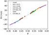 |
Fig. 4 Phase-folded diagram of the RV measurements relative to the spectra used for the extraction of the planetary CCF (Sect. 5) and grouped by instrument as listed in Table 3. Uncertainties are smaller than the symbol size. Phase 0 corresponds to the inferior conjunction of the planet. |
Spectral ranges excluded in the computation of the CCF.
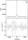 |
Fig. 5 Example of the test discussed in the text. Top panel: comparison between the individual CCF and the average CCF of the simulated stellar spectra. Bottom panel: normalization of the CCF shown in the top panel. The dashed smooth line shows the expected noiseless signal as in Eq. (19), thus marking the position of the injected planetary CCF. |
5.2 Analysis of real datasets
The simulation discussed so far proves that our method is able to robustly extract the planetary signal claimed by Martins et al. (2015) and Borra & Deschatelets (2018). We now want to replicate their detection using the large set of spectra we have collected (Table 1). The result of our analysis is shown in Fig. 7. The most striking piece of evidence is that we did not find any signals at the expected Kp ≃ 132 km s−1 above noise. For the sake of comparison with Martins et al. (2015) and Borra & Deschatelets (2018), in Fig. 7 we also plotted the result of our method applied only to the dataset taken on 2013 September 30. Once again, we did not find any evident signal above noise, which is now larger because we restricted the analysis to a smaller set of spectra.
We remark that, despite all the approaches make use of the CCF of the spectra, there are several differences. First of all, Martins et al. (2015) and Borra & Deschatelets (2018) excluded all the wavelength ranges affected by telluric contamination. Conversely, as discussed in Sect. 3, we carefully corrected the telluric absorption in the observed spectra and were therefore able to extend the wavelength range for analysis purposes. This actually has the effect of reducing the noise in the CCFs and would lead us to a more robust detection, as mentioned above. To make a closer comparison in this respect, we also performed our calculations excluding the ranges affected by telluric contamination in order to exclude the possibility that an imperfect telluric correction on our side might reduce the planetary signal. This is not the case, as this new analysis is consistent with the previous one within noise.
Secondly, we analyzed only a subset of the spectra taken for the 091.C-0271 program because the technique works best for spectra taken within a single night of observations. The reason is that the HARPS spectrograph is not designed to allow for the flux calibration of the observed spectra, nor is the reduction pipeline optimized to reduce the spectra at the 10−4 accuracy level on the flux. This may introduce some correlated noise in the continuum of the CCF (Fig. 5). The first word ofcaution is that these effects may vary from night to night, depending on the quality of the afternoon calibration or on the thermo-mechanical parameters of the telescope, for example. It is thus safer from this point of view to restrict the phase-resolved spectroscopic analysis within each individual night of observation.
As a matter of fact, during a given night, the Doppler shift of the stellar spectrum is less than one pixel or, in other words, the stellar spectra have a negligible Doppler shift in pixel coordinates. This means that any kind of uncorrected feature in the observed spectra does not move in wavelength with respect to the stellar spectrum. This leads to the presence of a correlated pattern in the continuum of the CCFs, which does not drift in velocity space from one observation to the other. The same pattern is then propagated in the computation of the average CCF. The normalization step (Eq. (16)) thus guarantees the correction of the correlated noise in the continuum. If several nights of observations are combined to compute the average stellar spectrum, then the result is unpredictable as it depends on how the instrumental setup has evolved and which orbital phases have been sampled.
One possibility to minimize the systematic errors is to compare the spectra taken during two consecutive nights. In Fig. 8 we show the result of our analysis restricted to the night of 2017 July 27 using either the average spectrum of the same night or the one corresponding to the night of 2017 July 26. In the second case, we obtain a trend which is likely due to mismatches in the spectral normalization between the two nights, while the correlated noise on top of the trend does not increase significantly.
This test also leads to another important piece evidence. In Sect. 2 we show that the planetary signal in the average CCF is diluted and reduced in amplitude by the median-average. The dilution leads to a valley in the normalized individual CCFs at the same radial velocities of the planet in the stellar rest frame (Fig. 1). This valley partially reduces the amplitude of the planetary signal, down to the noise level in a pessimistic scenario. To maximize the planetary CCF, one should thus use a reference CCF unaffected by the planetary signal in the velocity range of interest. The previous test aims to simulate such a scenario. As a matter of fact, we analyzed the spectra on the night of 2017 July 27 (i.e., after superior conjunction) using the master spectrum from the night of 2017 July 26 (i.e., before superior conjunction). With this combination of nights, we ensured that any residuals from the planetary signal in the reference CCF from the night of 2017 July 26 did not cover the velocity range encompassed by the expected planetary CCF on the night of 2017 July 27. Even in this case, where the interference of the planetary CCF with itself has been avoided, we would be able to detect the claimed planetary signal with a significance of ~ 4σ, but in fact we get negative results as shown in Fig. 8.
As a final test, given that we did not find any signatures of the planetary reflected spectrum, we assumed that the stellar spectra are not contaminated by the planet, and we injected a fake planetary spectrum in the spectra assuming Kp = 132 km s−1 and ɛmax = 10−4, as was donefor the simulations discussed earlier in this section. We find that the such a signal would be clearly detectable above noise in all the datasets in Table 1 and even better in the joint analysis (right panel in Fig. 7). In particular, the amplitude of the planetary signal would be ~ 3.6 and ~ 22 times larger than noise when we analyze the night 2013 September 30 and the full dataset, respectively.
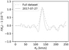 |
Fig. 6 Simulated |

 |
Fig. 7 Left panel: |

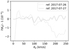 |
Fig. 8 Comparison of the analysis of the spectra taken on 2017 July 27 using the stellar template corresponding to the same night (solid line) and to the night of 2017 July 26. |
6 Discussion and conclusions
The first successful detection of the planetary spectrum of 51 Peg b was reported by Brogi et al. (2013), who discovered the absorption of carbon monoxide and water vapor in the CRIRES spectra of the dayside hemisphere. Analyzing the Doppler shift of the planetary spectra, the authors also put a constraint on the orbital inclination between 70°.6 and 82°.2 (with the upper limit set by the non-transiting nature of the planet), and they derived the planetary velocity amplitude Kp = 134.1 ± 1.8 km s−1. These measurements lead to a planetary mass of Mp = 0.46 ± 0.02 MJup. The same results were later corroborated by Birkby et al. (2017), who also estimated the rotational velocity of the planet to be vrot < 5.8 km s−1.
Likewise, Martins et al. (2015) analyzed the optical spectra of the 51 Peg system, looking for reflection by the planet. Using the CCF technique, they estimated the planetary velocity amplitude as 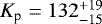 km s−1 and a corresponding planetary mass of
  , thus confirming the results of Brogi et al. (2013). The FWHM of the planetary CCF that they derived is ~ 23 ± 4 km s−1, which is significantly broader than the stellar CCF (FWHM = 7.43 km s−1). The authors caution that it can be due to the fact that the signal is close to the noise level. Nonetheless, if the broadening is confirmed, according to the authors, the broadening may indicate the rapid rotation of the planet (18 km s−1) much faster than the tidally locked rotation (2 km s−1). Strachan & Anglada-Escudé (2020) reproduced the same broadening using a more sophisticated model which accounts for the finite size of the star and planet in the integration of radiated and scattered flux intensities across both of their surfaces. Borra & Deschatelets (2018) improved the application of the CCF technique in the search of the reflected spectra, and they confirm the results of Martins et al. (2015). Moreover, they estimate a lower value for the FWHM of the planetary CCF, that is 9.69 ± 0.28 km s−1, which is much closer to the stellar FWHM, but still higher than predicted by Birkby et al. (2017).
In this paper, we analyze a larger set of HARPS and HARPS-N spectra of the 51 Peg planetary system taken when the planet was near superior conjunction. In our analysis, we were inspired by Martins et al. (2015) and Borra & Deschatelets (2018) in using the CCF technique as a powerful tool to extract weak signals buried in the noise. We detail the mathematical formalism about the CCF method tailored to the search of the light reflected by the planet, which we find to be only vaguely presented in the literature. We also describe how we reduced the data in order to optimize the extraction of the planetary signal. We checked that our method and data reduction were robust enough to allow for the detection of the signal claimed by Martins et al. (2015) and Borra & Deschatelets (2018). However, we do not find any evidence of the reflected planetary spectrum.
Including our reanalysis, there are thus two firm detections of the planetary reflected spectrum in the optical and two null detections. The two positive detections were obtained using similar techniques on the same dataset. The null detection by Di Marcantonio et al. (2019) was obtained on the same data but with a completely different mathematical approach, while our result isan extension of the CCF technique to a larger dataset. This opens the possibility that the detected signals may be caused by pitfalls of the technique coupled with the characteristics of the analyzed dataset. For this purpose, in Sect. 5 and Fig. 7, we present our algorithm that was run on the spectra collected on 2013 September 30, which include half of the spectra analyzed by Martins et al. (2015) and Borra & Deschatelets (2018). Even if this analysis does not return any significant signals, we notice a broad bump around ~ 150 km s−1 (left panel Fig. 7). This suggests the hypothesis that the claimed detection is just a false positive signal, unluckily located at the expected velocity Kp ~ 132 km s−1, and pushed up by a wicked combination of the properties of the CCF computation with the sampled planetary orbital phases.
The controversial point about the detection is the amplitude of the planetary signal (ɛmax = 12.5 × 10⁻⁵ and 8.6 × 10⁻⁵ as derived by Martins et al. 2015 and Borra & Deschatelets 2018, respectively). As a matter of fact, once the planet-to-star flux ratio ɛmax in Eq. (5) is fixed, there is an inverse proportionality between the geometric albedo Ag and the square of the planetary radius Rp. Based on observational evidence, Angerhausen et al. (2015) provide a typical value of Ag = 0.1 for the planetary albedo, which translates into a radius of ~3.9 RJup. Combining this predicted radius with the mass estimates provided by Brogi et al. (2013) and Birkby et al. (2017), we determined that the bulk density expected for 51 Peg b is 0.01 g cm−3, which puts 51 Peg b beyond the sample of H- and He-dominated, extremely low density planets (Laughlin 2018). This is a plausible yet unlikely scenario: for example, to date in the Exoplanet Orbit Database (Han et al. 2014), there is only one HJ (HAT-P-65 b, Hartman et al. 2016) out of 245 which are less dense than 0.15 g cm−3, while the planets with the lowest density ever measured (0.03 g cm−3) are the bloated Jupiter-sized Earth-mass planets Kepler51 b and c (Masuda 2014).
To reconcile 51 Peg b with the general properties of HJs, one can allow higher albedos and make the corresponding planetary radii smaller. For example, following Fig. 2 in Laughlin (2018) and converting densities into radii, we can assume that the maximum radius of an HJ with the same mass as 51 Peg b is 1.5 RJup. Inverting Eq. (5) and adopting the ɛmax derived by Martins et al. (2015), the corresponding planetary albedo would be Ag ≃ 0.68. For the sake of comparison, the highest albedo reported by Angerhausen et al. (2015) is Ag = 0.32, that is to say even the largest radius expected for 51 Peg b is not able to return a feasibly low geometric albedo.
Our analysis leads to a different scenario. Assuming that there is no trace of the planetary reflected spectrum in the data, Fig. 7 (left panel) represents the noise which limits our capability to detect the planetary CCF. After some injection and retrieval experiments, we find that the minimum signal that we can detect above the 3σ level corresponds to ɛmax = 10−5, which thus represents the upper limit for the planet-to-star flux ratio. In Fig. 9 we compare this detection limit with the ɛmax expected for 51 Peg b. In particular, following Laughlin (2018), we assume that an HJ with the same mass as 51 Peg b has a radius in the 0.9–1.5 RJup range. Afterinserting these radius limits in Eq. (5), we plotted the corresponding ɛmax versus Ag relations in Fig. 9. We find that an albedo of Ag = 0.1 corresponds to ɛmax between 6 × 10⁻⁶ and 2 × 10⁻⁵, which is close to our detection limit. We thus conclude that our null detection is consistent with a dark (Ag < 0.1) average-sized HJ and that 51 Peg b is not an outlier in terms of albedo and/or planetary radius. This result is consistent with the theoretical predictions provided by Sudarsky et al. (2000): in the upper atmosphere of an HJ-like 51 Peg b, the dominant contributionto the opacity is given by the broad absorption of alkali metals (Na, K), which precludes the silicate clouds at deeper layers from leading to a significant albedo.
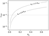 |
Fig. 9 ɛmax versus Ag relationship,as in Eq. (5), assuming Rp = 0.9 RJup and Rp= 1.5 RJup. The dashes represent our upper limit on ɛmax. |
Acknowledgements
This research has made use of the Exoplanet Orbit Database and the Exoplanet Data Explorer at exoplanets.org. G.Sc. acknowledges his niece M.Ma. for delighting her proud uncle during the writing of this paper. G.Sc., F.Bo., G.Br., I.Pa. and G.Pi. acknowledge the funding support from Italian Space Agency (ASI) regulated by “Accordo ASI-INAF n. 2013-016-R.0 del 9 luglio 2013 e integrazione del 9 luglio 2015”. G.Br. acknowledges support from CHEOPS ASI-INAF agreement n. 2019-29-HH.0. M.Es. acknowledges the support of the DFG priority program SPP 1992 “Exploring the Diversity of Extrasolar Planets” (HA 3279/12-1).
References
- Angerhausen, D., DeLarme, E., & Morse, J. A. 2015, PASP, 127, 1113 [NASA ADS] [CrossRef] [Google Scholar]
- Birkby, J. L., de Kok, R. J., Brogi, M., et al. 2017, AJ, 153, 138 [NASA ADS] [CrossRef] [Google Scholar]
- Borra, E. F., & Deschatelets, D. 2018, MNRAS, 481, 4841 [NASA ADS] [CrossRef] [Google Scholar]
- Bressan, A., Marigo, P., Girardi, L., et al. 2012, MNRAS, 427, 127 [NASA ADS] [CrossRef] [Google Scholar]
- Brogi, M., Snellen, I. A. G., de Kok, R. J., et al. 2012, Nature, 486, 502 [Google Scholar]
- Brogi, M., Snellen, I. A. G., de Kok, R. J., et al. 2013, ApJ, 767, 27 [NASA ADS] [CrossRef] [Google Scholar]
- Brogi, M., Line, M., Bean, J., et al. 2017, ApJ, 839, L2 [NASA ADS] [CrossRef] [Google Scholar]
- Charbonneau, D., Noyes, R. W., Korzennik, S. G., et al. 1999, ApJ, 522, L145 [NASA ADS] [CrossRef] [Google Scholar]
- Charbonneau, D., Brown, T. M., Noyes, R. W., et al. 2002, ApJ, 568, 377 [NASA ADS] [CrossRef] [Google Scholar]
- Claudi, R., Benatti, S., Carleo, I., et al. 2017, EpJ, 132, 364 [NASA ADS] [Google Scholar]
- Collier Cameron, A., Horne, K., Penny, A., et al. 1999, Nature, 402, 751 [NASA ADS] [CrossRef] [Google Scholar]
- Cosentino, R., Lovis, C., Pepe, F., et al. 2012, Proc. SPIE, 8446, 84461V [Google Scholar]
- Covino, E., Esposito, M., Barbieri, M., et al. 2013, A&A, 554, A28 [NASA ADS] [CrossRef] [EDP Sciences] [Google Scholar]
- Cowan, N. B.,& Agol, E. 2011, ApJ, 729, 54 [NASA ADS] [CrossRef] [Google Scholar]
- da Silva, L., Girardi, L., Pasquini, L., et al. 2006, A&A, 458, 609 [NASA ADS] [CrossRef] [EDP Sciences] [Google Scholar]
- Deming, D., & Knutson, H. A. 2020, Nat. Astron., 4, 453 [NASA ADS] [CrossRef] [Google Scholar]
- Di Marcantonio, P., Morossi, C., Franchini, M., et al. 2019, AJ, 158, 161 [CrossRef] [Google Scholar]
- Fuhrmann, K., Pfeiffer, M. J., & Bernkopf, J. 1997, A&A, 326, 1081 [NASA ADS] [Google Scholar]
- Gaia Collaboration (Brown, A. G. A., et al.) 2018, A&A, 616, A1 [NASA ADS] [CrossRef] [EDP Sciences] [Google Scholar]
- Garhart, E., Deming, D., Mandell, A., et al. 2020, AJ, 159, 137 [NASA ADS] [CrossRef] [Google Scholar]
- Goodman, J., & Weare, J. 2010, Commun. Appl. Math. Comput. Sci., 5, 65 [Google Scholar]
- Guilluy, G., Andretta, V., Borsa, F., et al. 2020, A&A, 639, A49 [EDP Sciences] [Google Scholar]
- Hartman, J. D., Bakos, G. Á., Bhatti, W., et al. 2016, AJ, 152, 182 [NASA ADS] [CrossRef] [Google Scholar]
- Han, E., Wang, S. X., Wright, J. T., et al. 2014, PASP, 126, 827 [NASA ADS] [CrossRef] [Google Scholar]
- Heng, K., & Demory, B.-O. 2013, ApJ, 777, 100 [NASA ADS] [CrossRef] [Google Scholar]
- Hilditch, R. W. 2001, An Introduction to Close Binary Stars (Cambridge Cambridge University Press) [CrossRef] [Google Scholar]
- Hoeijmakers, H. J., Snellen, I. A. G., & van Terwisga, S. E. 2018, A&A, 610, A47 [NASA ADS] [CrossRef] [EDP Sciences] [Google Scholar]
- Hyvärinen, A., Karhunen, J., & Oja, E. 2001, Independent Component Analysis (New York: John Wiley & Sons) [CrossRef] [Google Scholar]
- Kausch, W., Noll, S., Smette, A., et al. 2015, A&A, 576, A78 [NASA ADS] [CrossRef] [EDP Sciences] [Google Scholar]
- Kreidberg, L., Line, M. R., Parmentier, V., et al. 2018, AJ, 156, 17 [NASA ADS] [CrossRef] [Google Scholar]
- Laughlin, G. 2018, Handbook of Exoplanets (Cham: Springer), 1 [Google Scholar]
- Lo Curto, G., Pepe, F., Avila, G., et al. 2015, The Messenger, 162, 9 [NASA ADS] [Google Scholar]
- Lucy, L. B., & Sweeney, M. A. 1971, AJ, 76, 544 [NASA ADS] [CrossRef] [Google Scholar]
- Malavolta, L., Nascimbeni, V., Piotto, G., et al. 2016, A&A, 588, A118 [NASA ADS] [CrossRef] [EDP Sciences] [Google Scholar]
- Mallonn, M., Nascimbeni, V., Weingrill, J., et al. 2015, A&A, 583, A138 [NASA ADS] [CrossRef] [EDP Sciences] [Google Scholar]
- Mancini, L., Southworth, J., Raia, G., et al. 2017, MNRAS, 465, 843 [NASA ADS] [CrossRef] [Google Scholar]
- Martins, J. H. C., Figueira, P., Santos, N. C., et al. 2013, MNRAS, 436, 1215 [NASA ADS] [CrossRef] [Google Scholar]
- Martins, J. H. C., Santos, N. C., Figueira, P., et al. 2015, A&A, 576, A134 [NASA ADS] [CrossRef] [EDP Sciences] [Google Scholar]
- Masuda, K. 2014, ApJ, 783, 53 [Google Scholar]
- Mayor, M., & Queloz, D. 1995, Nature, 378, 355 [Google Scholar]
- Mayor, M., Queloz, D., Marcy, G., et al. 1995, IAU Circ., 6251 [Google Scholar]
- Murgas, F., Pallé, E., Parviainen, H., et al. 2017, A&A, 605, A114 [NASA ADS] [CrossRef] [EDP Sciences] [Google Scholar]
- Naef, D., Mayor, M., Beuzit, J. L., et al. 2004, A&A, 414, 351 [NASA ADS] [CrossRef] [EDP Sciences] [Google Scholar]
- Nascimbeni, V., Piotto, G., Pagano, I., et al. 2013, A&A, 559, A32 [NASA ADS] [CrossRef] [EDP Sciences] [Google Scholar]
- Nascimbeni, V., Mallonn, M., Scandariato, G., et al. 2015, A&A, 579, A113 [NASA ADS] [CrossRef] [EDP Sciences] [Google Scholar]
- Parmentier, V., & Crossfield, I. J. M. 2018, Handbook of Exoplanets (Cambridge: Cambridge University Press), 116 [Google Scholar]
- Perryman, M. 2018, The Exoplanet Handbook (Cambridge: Cambridge University Press) [Google Scholar]
- Pino, L., Ehrenreich, D., Wyttenbach, A., et al. 2018, A&A, 612, A53 [NASA ADS] [CrossRef] [EDP Sciences] [Google Scholar]
- Pino, L., Désert, J.-M., Brogi, M., et al. 2020, ApJ, 894, L27 [Google Scholar]
- Rodrigues, T. S., Girardi, L., Miglio, A., et al. 2014, MNRAS, 445, 2758 [Google Scholar]
- Rodrigues, T. S., Bossini, D., Miglio, A., et al. 2017, MNRAS, 467, 1433 [NASA ADS] [Google Scholar]
- Santos, N. C., Sousa, S. G., Mortier, A., et al. 2013, A&A, 556, A150 [NASA ADS] [CrossRef] [EDP Sciences] [Google Scholar]
- Sing, D. K., Désert, J.-M., Lecavelier Des Etangs, A., et al. 2009, A&A, 505, 891 [NASA ADS] [CrossRef] [EDP Sciences] [Google Scholar]
- Sing, D. K., Fortney, J. J., Nikolov, N., et al. 2016, Nature, 529, 59 [Google Scholar]
- Singh, V., Bonomo, A. S., Cibrario, N., et al. 2020, A&A, submitted [Google Scholar]
- Skrutskie, M. F., Cutri, R. M., Stiening, R., et al. 2006, AJ, 131, 1163 [NASA ADS] [CrossRef] [Google Scholar]
- Smette, A., Sana, H., Noll, S., et al. 2015, A&A, 576, A77 [NASA ADS] [CrossRef] [EDP Sciences] [Google Scholar]
- Snellen, I. A. G., de Kok, R. J., de Mooij, E. J. W., et al. 2010, Nature, 465, 1049 [Google Scholar]
- Sokal, A. 1997, Functional Integration: Basics and Applications (New York: Springer), 131 [Google Scholar]
- Sotzen, K. S., Stevenson, K. B., Sing, D. K., et al. 2020, AJ, 159, 5 [NASA ADS] [CrossRef] [EDP Sciences] [Google Scholar]
- Sousa, S. G., Adibekyan, V., Delgado-Mena, E., et al. 2018, A&A, 620, A58 [NASA ADS] [CrossRef] [EDP Sciences] [Google Scholar]
- Strachan, J. B. P., & Anglada-Escudé, G. 2020, MNRAS, 493, 1596 [Google Scholar]
- Sudarsky, D., Burrows, A., & Pinto, P. 2000, ApJ, 538, 885 [Google Scholar]
- Sudarsky, D., Burrows, A., & Hubeny, I. 2003, ApJ, 588, 1121 [Google Scholar]
- Stevenson, K. B., Désert, J.-M., Line, M. R., et al. 2014, Science, 346, 838 [Google Scholar]
- Vidal-Madjar, A., Désert, J.-M., Lecavelier des Etangs, A., et al. 2004, ApJ, 604, L69 [Google Scholar]
- Vissapragada, S., Knutson, H. A., Jovanovic, N., et al. 2020, AJ, 159, 278 [Google Scholar]
- Wakeford, H. R., Lewis, N. K., Fowler, J., et al. 2019, AJ, 157, 11 [Google Scholar]
- Walker, G. A.H., Matthews, J. M., Kuschnig, R., et al. 2006, in Tenth Anniversary of 51 Peg-b: Status of and Prospects for Hot Jupiter Studies, eds. L. Arnold, F. Bouchy, & C. Moutou (Paris: Frontier), 267 [Google Scholar]
- Welbanks, L., Madhusudhan, N., Allard, N. F., et al. 2019, ApJ, 887, L20 [CrossRef] [Google Scholar]
Borra & Deschatelets (2018) use the nomenclature auto-correlation function (ACF) in their work. Strictly speaking, the ACF is the cross-correlation of a signal with a copy of itself. What they actually computed, though, was the cross-correlation of the spectra with a stellar template, which was obtained as the average of a list of spectra. This is why we prefer to keep the wording CCF in the rest of our work.
All Tables
All Figures
|
Fig. 1 Expected planetary signal as discussed in the text. Different orbital phases approaching superior conjunction are simulated, as annotated in the plot. The parameters adopted for the simulations are ɛmax = 10−4, σ = 10.6 km s−1, A = 3000, and δ = 1000 (Eq. (16)), together with the orbital solution derived in Sect. 4. |
| In the text | |
|
Fig. 2 Example of the result of the telluric correction discussed in the text. |
| In the text | |
|
Fig. 3 Phase-folded diagram of the analyzed RV measurements using the ephemeris listed in Table 3 (top panel) and corresponding residuals (bottom panel). Measurements from different instruments are marked with different symbols as shown in the legend. The “Lick6,” “Lick8,” and “Lick13” labels are the same as in Birkby et al. (2017) and denote the dewar associated with the spectrograph in use during the observations. Phase 0 corresponds to the inferior conjunction of the planet. |
| In the text | |
|
Fig. 4 Phase-folded diagram of the RV measurements relative to the spectra used for the extraction of the planetary CCF (Sect. 5) and grouped by instrument as listed in Table 3. Uncertainties are smaller than the symbol size. Phase 0 corresponds to the inferior conjunction of the planet. |
| In the text | |
|
Fig. 5 Example of the test discussed in the text. Top panel: comparison between the individual CCF and the average CCF of the simulated stellar spectra. Bottom panel: normalization of the CCF shown in the top panel. The dashed smooth line shows the expected noiseless signal as in Eq. (19), thus marking the position of the injected planetary CCF. |
| In the text | |
|
Fig. 6 Simulated |
| In the text | |
|
Fig. 7 Left panel: |
| In the text | |
|
Fig. 8 Comparison of the analysis of the spectra taken on 2017 July 27 using the stellar template corresponding to the same night (solid line) and to the night of 2017 July 26. |
| In the text | |
|
Fig. 9 ɛmax versus Ag relationship,as in Eq. (5), assuming Rp = 0.9 RJup and Rp= 1.5 RJup. The dashes represent our upper limit on ɛmax. |
| In the text | |
Current usage metrics show cumulative count of Article Views (full-text article views including HTML views, PDF and ePub downloads, according to the available data) and Abstracts Views on Vision4Press platform.
Data correspond to usage on the plateform after 2015. The current usage metrics is available 48-96 hours after online publication and is updated daily on week days.
Initial download of the metrics may take a while.