| Issue |
A&A
Volume 646, February 2021
|
|
|---|---|---|
| Article Number | A43 | |
| Number of page(s) | 10 | |
| Section | Planets and planetary systems | |
| DOI | https://doi.org/10.1051/0004-6361/202038870 | |
| Published online | 05 February 2021 | |
Coexistence of CH4, CO2, and H2O in exoplanet atmospheres
1
Centre for Exoplanet Science, University of St Andrews,
St Andrews, UK
e-mail: This email address is being protected from spambots. You need JavaScript enabled to view it.
2
SUPA, School of Physics & Astronomy, University of St Andrews,
St Andrews, KY16 9SS, UK
3
School of Earth & Environmental Studies, University of St Andrews,
St Andrews, KY16 9AL, UK
4
SRON Netherlands Institute for Space Research,
Sorbonnelaan 2,
3584 CA Utrecht, The Netherlands
Received:
8
July
2020
Accepted:
17
October
2020
Abstract
We propose a classification of exoplanet atmospheres based on their H, C, O, and N element abundances below about 600 K. Chemical equilibrium models were run for all combinations of H, C, O, and N abundances, and three types of solutions were found, which are robust against variations of temperature, pressure, and nitrogen abundance. Type A atmospheres contain H2O, CH4, NH3, and either H2 or N2, but only traces of CO2 and O2. Type B atmospheres contain O2, H2O, CO2, and N2, but only traces of CH4, NH3, and H2. Type C atmospheres contain H2O, CO2, CH4, and N2, but only traces of NH3, H2, and O2. Other molecules are only present in ppb or ppm concentrations in chemical equilibrium, depending on temperature. Type C atmospheres are not found in the Solar System, where atmospheres are generally cold enough for water to condense, but exoplanets may well host such atmospheres. Our models show that graphite (soot) clouds can occur in type C atmospheres in addition to water clouds, which can occur in all types of atmospheres. Full-equilibrium condensation models show that the outgassing from warm rock can naturally provide type C atmospheres. We conclude that type C atmospheres, if they exist, would lead to false positive detections of biosignatures in exoplanets when considering the coexistence of CH4 and CO2, and suggest other, more robust non-equilibrium markers.
Key words: planets and satellites: atmospheres / planets and satellites: composition / planets and satellites: physical evolution / astrochemistry
© ESO 2021
1 Introduction
The detection of exoplanets that exhibit spectral signatures of biological activity (biosignatures) is one of the most urgent goals of modern astronomy. Because of observational limitations, such biosignatures are currently based on certain combinations of abundant molecules that exhibit detectable spectroscopic signatures at medium spectral resolution in the infrared, such as H2O, CO2, CH4, and CO. Other potentially abundant molecules like H2, O2, and N2 have no permanent dipole moment and are more difficult to detect. Molecules generally need to have a minimum concentration of about 10−4 (100 ppm) to be detectable with the James Webb Space Telescope (JWST; Krissansen-Totton et al. 2019; Sousa-Silva et al. 2020), and a number of candidates have recently been discussed. For example, O3 as an indicator for the presence of O2 (Gaudi et al. 2018), SO2-derived sulphate aerosols as an indicator for volcanic activity (Misra et al. 2015), and PH3 as a biosignature (Sousa-Silva et al. 2020).
Searching for suitable combinations of detectable molecules that suggest biological activity, Krissansen-Totton et al. (2019) recently proposed to consider the coexistence of CO2 and CH4 (without CO) in planetary atmospheres. CO2 and CH4 represent the two endpoints of the redox-spectrum of carbon, yet both molecules are present in the Earth atmosphere (Meadows et al. 2018). Krissansen-Totton et al. (2018) argued that a disequilibrium between CH4 and CO2, accompanied by N2 and liquid H2O, was present during the Archean on Earth. Sandora & Silk (2020) review the evolutionary processes involving CH4 in the atmosphere of Earth. Once the specific geological processes that used to cause that disequilibrium cease, it seems unlikely that non-biological processes could maintain such an atmosphere on habitable exoplanets. However, Krissansen-Totton et al. did not explore the extent to which CO2 and CH4 can simply coexist in chemical equilibrium.
Previous chemical models in astronomy have mainly focused on H-rich atmospheres. For example, Moses et al. (2013) and Hu & Seager (2014) presented sparse grids of chemical models varying the H abundance, metallicity, and C/O-ratio to study the atmospheric composition of mini Neptunes and super Earths, including kinetical quenching, photodissociation, and vertical mixing. These papers show that carbon can mostly form CO2 at low H abundances, rather than CO and CH4 as used from the H2-dominated atmospheres. Heng & Tsai (2016) considered an analytic nine-molecule model in chemical equilibrium to discuss the effects of varying C/O and N/O ratios on H2-dominated hot exoplanet atmospheres, aiming to develop a fast tool to retrieve the atmospheric composition from exoplanet observations. Morley et al. (2017) considered chemical equilibrium models for the atmospheres of Earth-sized exoplanets, including those of the TRAPPIST-1 system, based on element abundances taken from Venus, Earth, and Titan to discuss their observability with JWST.
Simulating the chemical evolution of the atmosphere on Earth, (Zerkle et al. 2012) identified the photo-dissociation of CH4 as an important non-equilibrium physical process in the upper atmosphere. The low dissociation energy of CH4 (~ 4.3 eV) implies that this molecule can be dissociated quite easily compared to CO2. Therefore, UV irradiation is thought to significantly change the atmospheric CH4 /CO2 ratio over time (Zerkle et al. 2012), and if the hydrogen atoms (or H2 molecules) produced by this reaction can escape, the photo-dissociation of CH4 is able to remove hydrogen from exoplanet atmospheres, creating more oxidising conditions. Arney et al. (2016) proposed that during the Archean, Earth was likely covered in a photochemical haze triggered by this process. Another large uncertainty here is the Earth’s history of surface pressure and atmospheric N2 abundance, which was possibly affected by the evolution of life as well (Stüeken et al. 2016).
The aim of this paper is to present an exhaustive study of the composition of exoplanet atmospheres considering all possible combinations of H, C, O, and N abundances assuming chemical equilibrium. Substantial deviations from chemical equilibrium can be caused by biological activity, but other physical and geological processes may explain these disequilibria, too, for example UV and cosmic ray irradiation. Nevertheless, potential biosignatures should not be based on combinations of molecules that are already expected in chemical equilibrium (Seager et al. 2013).
Atomisation energies Ea of selected molecules.
2 Simplified chemical equilibrium
All known atmospheres of Solar-System bodies are mainly composed of hydrogen (H), carbon (C), oxygen (O), and nitrogen (N), so we focus on the H–C–O–N system in this paper, which is the most pressing system for the observational characterisation of exoplanets and the identification of possible biosignatures.
At low temperatures, T ≲ 600 K, the Gibbs free energies ΔGf = ΔHf − TΔS are dominated by the enthalpy of formation ΔHf, which means that in chemical equilibrium, the molecular concentrations will essentially minimise ΔHf. In Table 1 we list a few atomisation energies, that is, the energies required to convert molecules into neutral atoms; for example Ea (H2O) = 2ΔHf(H) + ΔHf(O) − ΔHf(H2O). The data were extracted from the NIST-Janaf tables (Chase et al. 1982; Chase 1986).
Simple combinatorics shows that CH4, CO2, H2 O, and N2 are the thermodynamically most favourable molecules to minimise ΔHf. For example, all of the following reactions are exothermic
![Mathematical equation: \begin{equation*} \hspace*{-4pt}\begin{array}{lcll} {\textrm{H}_2} + \frac{1}{4}\;{\textrm{CO}_2} &\longrightarrow& \frac{1}{2}\;{\textrm{H}_2\textrm{O}} + \frac{1}{4}\;{\textrm{CH}_4} &:\rm -0.39\,eV\\[0.8mm] \textrm{CO} + \frac{1}{2}\;{\textrm{H}_2\textrm{O}} &\longrightarrow& \frac{3}{4}\;{\textrm{CO}_2} + \frac{1}{4}\;{\textrm{CH}_4} &:\rm -0.81\,eV\\[0.8mm] \textrm{HCN} + \frac{3}{4}\;{\textrm{H}_2\textrm{O}} &\longrightarrow& \frac{3}{8}\;{\textrm{CO}_2} + \frac{5}{8}\;{\textrm{CH}_4} + \frac{1}{2}\;{\textrm{N}_2} &:\rm -1.51\,eV\\[0.8mm] {\textrm{C}_2\textrm{H}_2} + \frac{3}{2}\;{\textrm{H}_2\textrm{O}} &\longrightarrow& \frac{3}{4}\;{\textrm{CO}_2} + \frac{5}{4}\;{\textrm{CH}_4} &:\rm -2.56\,eV\\[0.8mm] {\textrm{NH}_3} + \frac{3}{8}\;{\textrm{CO}_2} &\longrightarrow& \frac{3}{4}\;{\textrm{H}_2\textrm{O}} + \frac{3}{8}\;{\textrm{CH}_4} + \frac{1}{2}\;{\textrm{N}_2} &:\rm -2.83\,eV\\[0.8mm] {\textrm{O}_2} + \frac{1}{2}\;{\textrm{CH}_4} &\longrightarrow& \;\;\;{\textrm{H}_2\textrm{O}} + \frac{1}{2}\;{\textrm{CO}_2} &:\textrm{-4.17\,eV} \end{array} \end{equation*}](/articles/aa/full_html/2021/02/aa38870-20/aa38870-20-eq1.png)
which means that all other molecules can react exothermally to eventually form a mixture of only CH4, CO2, H2 O, and N2 to minimise the Gibbs free energy at low temperatures. The first reaction requires that a C–O bond is broken, which is likely biologically mediated, and has been named “methanogenesis” by Woese & Fox (1977) and Waite et al. (2017). With increasing temperature, entropy becomes more relevant, and H2 is the first among the trace molecules to reach significant concentrations, followed by CO.
Therefore, we first consider a planetary atmosphere in which the most abundant molecules are H2 O, CH4, CO2, and N2 (hereafter referred to as type C atmospheres), such that the total gas pressure is approximately given by
 (1)
(1)
The elementconservation equations can be expressed in terms of a fictitious total pressure after complete atomisation, patom, here patom = 3 pH 2O + 5 pCH 4 + 3 pCO 2 + 2 pN 2,
![Mathematical equation: \begin{eqnarray} \textrm{H}\cdotp_{\textrm{atom}} ~=~ 2\,\pH2O + 4\,\pCH4&\!\!,& \textrm{C}\cdotp_{\textrm{atom}} ~=~ \pCO2 + \pCH4,\\[-0.5mm] \textrm{O}\cdotp_{\textrm{atom}} ~=~ \pH2O + 2\,\pCO2\hspace*{2mm} &\!\!\!\!\!\!\!\!\!,& \textrm{N}\cdotp_{\textrm{atom}} ~=~ 2\,\pN2,\end{eqnarray}](/articles/aa/full_html/2021/02/aa38870-20/aa38870-20-eq3.png)
where H, C, O, and N are the given element abundances normalised by the condition H + C + O + N = 1. The usual element abundances in astronomy are defined with respect to hydrogen, for example ϵC = C/H and ϵO = O/H, but here we wish to also consider hydrogen-poor atmospheres with H → 0.
This system of linear equations, Eqs. (1) to (3), can be readily solved for the molecular partial pressures
![Mathematical equation: \begin{equation*} \hspace*{-6pt}\begin{array}{lcc} \displaystyle \frac{\pH2O}{p_{\textrm{gas}}} = \frac{\textrm{H}+2\,\textrm{O}-4\,\textrm{C}}{\textrm{H}+2\,\textrm{O}+2\,\textrm{N}} &\hspace*{-6.6mm},\hspace*{-1mm}& \displaystyle \frac{\pCO2}{p_{\textrm{gas}}} = \frac{2\,\textrm{O}+4\,\textrm{C}-\textrm{H}}{2\,\textrm{H}+4\,\textrm{O}+4\,\textrm{N}},\\[4mm] \displaystyle \frac{\pCH4}{p_{\textrm{gas}}} = \frac{\textrm{H}-2\,\textrm{O}+4\,\textrm{C}}{2\,\textrm{H}+4\,\textrm{O}+4\,\textrm{N}} &\hspace*{-3.5mm},\hspace*{-1mm}&\hspace*{-0.7mm} \displaystyle \frac{\pN2}{p_{\textrm{gas}}} = \frac{2\,\textrm{N}}{\textrm{H}+2\,\textrm{O}+2\,\textrm{N}}.\end{array} \end{equation*}](/articles/aa/full_html/2021/02/aa38870-20/aa38870-20-eq4.png) (4)
(4)
If any of thepartial pressures according to Eq. (4) are negative, we have left the region of applicability of our assumptions. These side conditions are

We can furthermore use Eq. (4) to determine where two of the molecular partial pressures are equal

The partial pressure of N2 is always positive according to Eq. (4), providing no additional constraints. Hence, nitrogen does not interfere with the H–C–O system; unless there is a surplus of H according to Eq. (6), in whichcase NH3 becomes an abundant molecule; see Sect. A.1.
3 Full-chemical-equilibrium models
To confirm the simplified analysis presented in Sect. 2, we ran full-gas-phase-chemical-equilibrium models with GGCHEM (Woitke et al. 2018) for the elements H, C, N, and O. GGCHEM finds 52 molecular species in its database for this element mixture: H2, C2, N2, O2, CH, NH, OH, CN, CO, NO, HCN, CHNO, HCO, CH2, H2 CO, CH3, CH4, CNO, CNN, NCN, CO2, C2 H, C2 H2, C2 H4, C2 H4O, C2 N, C2 N2, C2 O, C3, C3 O2, C4, C4 N2, C5, HNO, HONO, HNO2, HNO3, HO2, NH2, N2 H2, H2 O, NH3, N2 H4, NO2, NO3, N2 O, N2 O3, N2 O4, N2 O5, N3, O3, and C3 H. The results for T = 400 K and p = 1 bar are shown in Fig. 1. The region of coexistence of H2O, CO2, and CH4 is indicated bya grey triangle corresponding to Eqs. (5)–(7), and the dashed lines of equal concentration correspond to Eqs. (8)–(10). The models have been computed with a small nitrogen abundance N = 10−3, but the results are independentof N when plotted as a function of C∕(H + O + C) and (O −H)∕(O + H) because nitrogen does not significantly interfere with the H–C–O system. See Appendix A for a discussion in how far our results depend on temperature, pressure, and nitrogen abundance.
These results show that indeed none of the other molecules are relevant to this problem. N2, H2 O, CO2, and CH4 are the onlymolecules that must be considered within the grey triangle to solve the element conservation equations, at least approximately, and therefore the argumentation presented in Sect. 2 holds.
The patterns shown in Fig. 1 are robust against changes of pressure, temperature, and nitrogen abundance; see Appendix A for details. This is the true strength of this diagram; all results can be approximately inferred simply from the identification and stoichiometry of the four most stable molecules, making these results suitable for a classification of exoplanet atmospheres. The central triangle shows trace concentrations of H2 on a level of a few 10−4 at 400 K; otherwise the gas composition is very pure in chemical equilibrium, with only three abundant molecules at any point besides N2. With increasing temperature, the H2 trace concentration increases, followed by the occurrence of CO in trace concentrations; see Table 2. Molecules not listed in Table 2 have even lower abundances. We conclude that the simplified analysis of the coexistence of H2 O, CO2, and CH4 as presentedin Sect. 2 is valid to about 600 K.
The results of Moses et al. (2013) and Hu & Seager (2014, see their Figs. 4–6) show similar patterns, but their sparse grid of models and usage of H-abundance and C/O ratio make it difficult to compare their results with ours in detail.
 |
Fig. 1 Molecular concentrations in chemical equilibrium as a function of H, C, and O element abundances, calculated for T = 400 K and p = 1 bar. The central grey triangle marks the region within which H2O, CH4, and CO2 coexist in chemical equilibrium. The thin grey lines indicate where two concentrations are equal: |


Trace gas concentrations in chemical equilibrium with element abundances N = 2∕13, H = 6∕13, O = 3∕13, and C = 2∕13, where the main constituents are 25% N2, 25% H2 O, 25% CO2, and 25% CH4.
4 Water and graphite condensation
GGCHEM also computes the supersaturation ratios of graphite C[s], liquid water H2 O[l], solid water H2 O[s], and the ices of ammonia NH3[s], methane CH4[s], CO[s], and CO2[s]. While the ices only deposit at T ≲ 200 K at 1 bar, the effect of carbon and water condensation is significant; see Fig. 2. Shaded areas in Fig. 2 indicate that at least one condensed species is supersaturated (S > 1). Such gases are expected to form clouds, and the precipitation of cloud particles would remove the respective elements from the gas phase. Exoplanet atmospheres cannot therefore reside within the shaded areas, but are expected to move toward the edges of the blank regions in Fig. 2, where they come to rest.
However, the extent of the supersaturated areas depends on temperature, pressure, and nitrogen abundance, and therefore on atmospheric height, which complicates the analysis. Earth, for example, is not a point in Fig. 2 but a line, because the water content in the gas phase increases with temperature, guided by the condition S(H2O, T) ≈ 1.
Figure 2 shows that at 350 K, 1 bar, and low nitrogen abundance, the triangle in which H2 O, CO2, and CH4 coexist is mostly covered by the supersaturated areas, either graphite or water or both. However, at 400 K water cannot condense anywhere in the left diagram, and then the grey triangle of coexistence is only partly inhibited by graphite condensation. The grey triangle is less affected by supersaturation for lower pressures or increased nitrogen abundances. The occurrence of graphite clouds in exoplanet atmospheres was discussed for example by Moses et al. (2013, see their Fig. 7).
Figure 3 shows the results of some full-equilibrium condensation models for 18 elements from Herbort et al. (2020). In these models, the total (= condensed + gas phase) element abundances are taken from different materials found in the Earth’s crust, meteorites, and polluted white dwarfs; see explanation of abbreviations in the figure caption. The model determines which liquid and solid materials are present at each temperature and subtracts the respective condensed element fractions until S ≤ 1 is achieved for all condensates. The remaining gas-phase element abundances are plotted in Fig. 3 with lines, where we start at 600 K (circle) and follow the results down to 200 K. The changes of the H, O, and C abundances along these tracks are caused by the effects of progressive condensation in these models, in particular phyllosilicates, carbonates, graphite, and water. The CC model is very dry and eventually creates an almost pure N2 atmosphere with some CO2 at low temperatures. All other models eventually form a mixture of N2 and CH4, similar to Titan’s atmosphere. In the MORB and BSE models, graphite condenses below 550and 600 K, respectively, but there is no liquid water. The PWD model shows neither graphite nor water condensation, but the CI and the water-enriched BSE models show liquid water at 369 and 373 K, respectively, below which the models follow tracks because of the removal of H2 O and C along the borderline between type A and C where the CO2-concentration is low but still notable; for example the CI model at 350 K has 10% N2, 48% CH4, 42% H2 O, and 0.35% CO2.
In Fig. 3, we additionally overplotted some simple equilibrium condensation models where only the four element H, C, O, and N are included. The initial element abundances of these models are arbitrarily set as listed in Table 3. These models show the principle behaviour of type A, B, and C atmospheres when only affected by water and graphite condensation. At ~ 350 K and 1 bar, the three type C models show similarabundances of CO2 and CH4, both with concentrations of a few percent, in addition to the major molecules N2 and H2 O, next to liquid water.
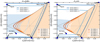 |
Fig. 2 Impact of liquid water (H2O) and graphite(C) condensation at constant pressure of 1 bar. The blue and orange contour lines mark where the supersaturation ratio S is equal to one for water and graphite, respectively, at selected temperatures. Inside of the light blue and light orange shaded regions, the gas is supersaturated with respect to water at 350 K and graphite at 500 K, respectively. For higher temperatures, lower pressures or higher N abundances, the shaded areas shrink and eventually vanish. The left diagram is calculated for a small nitrogen abundance N = 0.001, whereas N = 0.5 is assumed in the right diagram. The atmospheric compositions of Earth, Mars, Venus, Jupiter, Titan, and the Archean Earth (taken from Miller 1953) are marked. Earth (assuming 1.5% water content) sits right on top of the S(H2 O, 300 K, N = 0.5) = 1 line. |
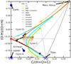 |
Fig. 3 Results from six full-equilibrium condensation models for 18 elements from Herbort et al. (2020) re-computed for p = 1 bar, and five simple models for just 4 elements; see Table 3. Each model starts at T = 600 K (marked by circles) and then we follow that model with a line down to 200 K with 200 log-equidistant points. Abbreviations are carbonaceous chondrites (CI), Mid Oceanic Ridge Basalt (MORB), Continental Crust (CC), Bulk Silicate Earth (BSE), and abundances deduced from polluted white dwarf (PWD) observations. The points where the trajectories start to have graphite are marked by crosses, and the points where liquid water starts to occur are marked by squares. |
5 Conclusions
We find thata mixture of H2O, CO2, CH4 and N2 is the most favourable combination of molecules to minimise the Gibbs free energy at low temperatures T ≲ 600 K. If all available elements can be converted into these molecules, the gas will only contain these species, whereas all other molecules only have trace concentrations in chemical equilibrium. However, if this is not possible because of stoichiometric constraints, additional types of atmospheres occur:
Setup of simple equilibrium condensation models for four elements.
- A)
Type A atmospheres are H-rich and mostly contain CH4, H2O, and NH3, but CO2 and O2 are lacking. In Appendix A.1 we show that the forth abundant molecule is either H2 (type A1) or N2 (type A2). The atmospheres of Jupiter, Titan, and Archean Earth belong to type A. Titan’s cold atmosphere is almost water-free because of condensation, but does have some H2 (about 0.15%, Niemann et al. 2005).
- B)
Type B atmospheres are O-rich and mostly contain O2, N2, CO2, and H2O, but CH4, NH3, and H2 are lacking. Earth belongs to this type. The Martian atmosphere is a member of type B, too, because it contains some O2 (about 0.1%1). Venus is too hot for our classification but its atmosphere is also mostly made of CO2 and N2, with traces of H2O, but no CH4 or NH31.
- C)
Type C atmospheres mostly contain H2O, CO2, CH4, and N2, but NH3, H2, and O2 are lacking. This type of atmosphere is discussed in Sect. 2.
The molecule CO is not abundant in any type of atmosphere at low temperatures in chemical equilibrium. Type C exoplanet atmospheres are not found in the Solar System, possibly because the low temperatures of the objects favour water condensation, which reduces the hydrogen and oxygen abundances; however, slightly warmer exoplanets may well host such atmospheres. Type C atmospheres are featured by the coexistence of CH4 and CO2, both with percent-concentrations, which is possible in equilibrium only in type C atmospheres. Our models furthermore suggest that only in type C atmospheres can carbon directly condense to form graphite (soot) clouds.
The fullequilibrium condensation models show that type C atmospheres can naturally be created by the outgassing from common rock materials such as carbonaceous chondrites (CI) or mid-oceanic-ridge basalt (MORB) at temperatures > 400 K. The two inner rocky planets of the Trappist-1 planet system, with estimated surface temperatures of about 370 and 320 K, respectively (Morley et al. 2017), might host such atmospheres, and will be observed with the JWST; see details in Turbet et al. (2020).
Biosignatures: the identification of spectral signatures of biological activity needs to proceed via two steps: first, identify combinations of molecules which cannot co-exist in chemical equilibrium (“non-equilibrium markers”). Second, find biological processes that cause such dis-equilibria, which cannot be explained by other physical non-equilibrium processes like photo-dissociation (“biosignatures”). The aim of this letter is to propose a robust criterion for step one. We define a non-equilibrium marker as a combination of (a) any given molecule with (b) one of H2 O, CH4, or CO2, such that molecules a and b can react exothermally to only produce H2O, CH4, CO2, and N2. Such pairs of molecules a and b populate the opposite corners in Fig. 1 and have practically zero overlap in equilibrium. Examples of such pairs of reactants in exothermal reactions are listed in Sect. 2.
Krissansen-Totton et al. (2019) proposed the simultaneous detection of CH4 and CO2 (without CO) as a biosignature, arguing that only biological fluxes are high enough to replenish CH4 in the upper atmospheres where it is rapidly destroyed by photochemical processes. However, the present study shows that CH4 and CO2 can coexist in chemical equilibrium in a type C atmosphere, which could lead to many false positive detections. The outgassing from warm common rocks provides a natural mechanism to generate equilibrated mixtures of CH4 and CO2 with only trace amounts of CO, and at T ≳ 400 K, type C atmospheres may contain equally large concentrations of H2O, CH4, and CO2 in chemical equilibrium. At T ≈ 350 K, liquid water can coexist with arbitrary concentrations of CH4 and a concentration of CO2 of the order of a few percent. It is important to re-evaluate photochemical effects in type C atmospheres, where there is no free oxygen available and therefore the reaction products of CH4 are more likely to simply reform CH4.
Acknowledgements
P. W. and Ch. H. acknowledge funding from the European Union H2020-MSCA-ITN-2019 under Grant Agreement no. 860470 (CHAMELEON). O. H. acknowledges the PhD stipend form the University of St Andrews’ Centre for Exoplanet Science. P. B. acknowledges support from the St Leonards interdisciplinary scholarship.
Appendix A Types A, B, and C atmospheres
In the following, we systematically list the principle molecular composition and approximate abundances expected for low-temperature gases in chemical equilibrium. These results are entirely given by the element abundances and the stoichiometric factors of the thermodynamically most favourable molecules, and are hence independent of pressure and temperature.
A.1 Type A atmospheres
Type A atmospheres are H-rich and occur for H > 2 O + 4 C (Eq. (6)). They are featured by the stability of NH3. Since N2 can react exothermally with H2
 (A.1)
(A.1)
we have either a combination of NH3 and H2 (type A1) or a combinationof NH3 and N2 (type A2), depending on nitrogen abundance.
Type A1atmospheres mainly contain H2O, CH4, NH3, and H2, and occur for H > 2 O + 4 C and low nitrogen abundance 3N < H − 2 O − 4 C. Based on the stoichiometry of these molecules, following the same procedure as outlined in Sect. 2 the expected low-temperature abundances in chemical equilibrium are
![Mathematical equation: \begin{equation*} \hspace*{-5pt}\begin{array}{lcc} \displaystyle \frac{\pH2O}{p_{\textrm{gas}}} = \frac{2\,\textrm{O}}{\textrm{H}-\textrm{N}-2\,\textrm{C}} &\hspace*{-3mm},\hspace*{-1mm}&\hspace*{-5mm} \displaystyle \frac{\pCH4}{p_{\textrm{gas}}} = \frac{2\,\textrm{C}}{\textrm{H}-\textrm{N}-2\,\textrm{C}} \,\\[4mm] \displaystyle \frac{\pNH3}{p_{\textrm{gas}}} = \frac{2\,\textrm{N}}{\textrm{H}-\textrm{N}-2\,\textrm{C}} &\hspace*{-3mm},\hspace*{-1mm}&\hspace*{2mm} \displaystyle \frac{{p_{\textrm{H}_{2}}}}{p_{\textrm{gas}}} = \frac{\textrm{H}-2\,\textrm{O}-4\,\textrm{C}-3\,\textrm{N}}{\textrm{H}-\textrm{N}-2\,\textrm{C}} \.\hspace*{-5mm}\end{array} \end{equation*}](/articles/aa/full_html/2021/02/aa38870-20/aa38870-20-eq9.png) (A.2)
(A.2)
Type A2 atmospheres mainly contain H2O, CH4, NH3, and N2, and occur for H > 2O + 4C and high nitrogen abundance 3N > H −2O − 4C. The expected low-temperature abundances in chemical equilibrium are
![Mathematical equation: \begin{equation*} \hspace*{-5pt}\begin{array}{lcc} \displaystyle \frac{\pH2O}{p_{\textrm{gas}}} = \frac{6\textrm{O}}{\textrm{H}+2\textrm{C}+3\textrm{N}+4\textrm{O}} &\hspace*{-5.8mm},\hspace*{-1mm}&\hspace*{0mm} \displaystyle \frac{\pCH4}{p_{\textrm{gas}}} = \frac{6\,\textrm{C}}{\textrm{H}+2\,\textrm{C}+3\,\textrm{N}+4\,\textrm{O}} \,\\[4mm] \displaystyle \frac{\pNH3}{p_{\textrm{gas}}} = \frac{2\,\textrm{H}-8\,\textrm{C}-4\,\textrm{O}}{\textrm{H}+2\,\textrm{C}+3\,\textrm{N}+4\,\textrm{O}} &\hspace*{-3mm},\hspace*{-1mm}&\hspace*{1mm} \displaystyle \frac{\pN2}{p_{\textrm{gas}}} = \frac{3\,\rm N+4\,C+2\,O-H}\textrm{H+2\,C+3\,N+4\,O} \.\end{array} \end{equation*}](/articles/aa/full_html/2021/02/aa38870-20/aa38870-20-eq10.png) (A.3)
(A.3)
Figure A.1 shows the concentrations of NH3, H2, and N2 in chemical equilibrium in type A atmospheres. The left parts of these plots, where (N −Heff)∕(N + Heff) < −0.5, correspond to type A1, and the right parts (N −Heff)∕(N + Heff) > −0.5 correspond to type A2. We used an effective H abundance here, Heff = H − 2 O − 4 C, in order to plot the results with regard to the hydrogen abundance still available after H2 O and CH4 formation. Comparison with a large sample of models, systematically varying all H, C, N, O abundances (see dots in Fig. A.1), showsthat the low-temperature expectations according to Eqs. (A.2) and (A.3) require temperatures T ≲ 300 K to be accurate, which differs from type B and type C atmospheres where the low-temperature expectations are accurate up to T ≲ 600 K. The reason for the earlier occurrence of deviations of the model results from their low-temperature expectations is that reaction (A.1) is only mildly exothermic, meaning that the entropy terms kick in sooner when increasing the temperature. Thus, the low-temperature expectations in type A atmospheres are far less useful as compared to type B and type C atmospheres, where they are more robust and hence more suitable for classification. However, the borderline between type C and type A atmospheres, and the prediction of H2 O and CH4 concentrations remains robust even in type A atmospheres.
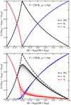 |
Fig. A.1 Concentrations of NH3, N2, and H2 in chemical equilibrium in type A atmospheres. Heff = H − 2 O − 4 C is the H element abundance remaining after subtraction of H2O and CH4. The dashedlines are the low-temperature expectations according to Eqs. (A.2) and (A.3). The dots are taken from a wide range of models, systematically varying the H, C, O, and N element abundances at p = 1 bar for T = 250 K (top plot) and for T = 350 K (bottom plot). |
Both type A1 and type A2 atmospheres can contain water clouds if temperatures are sufficiently low, but no graphite (soot) clouds and only traces of CO2, O2, and CO molecules in chemical equilibrium.
A.2 Type B atmospheres
Type B atmospheres are oxygen-rich and occur for 2 O > H + 4 C (Eq. (5)). They mainly contain H2O, CO2, N2, and O2. With similar stoichiometric arguments as presented in Sect. 2, the expected low-temperature abundances in chemical equilibrium are
![Mathematical equation: \begin{equation*} \begin{array}{lcc} \hspace*{-5pt}\displaystyle \frac{\pH2O}{p_{\textrm{gas}}} = \frac{2\,\textrm{H}}{\textrm{H}+2\,\textrm{O}+2\,\textrm{N}} &\hspace*{-2.8mm},\hspace*{-1mm}& \displaystyle \frac{\pCO2}{p_{\textrm{gas}}} = \frac{4\,\textrm{C}}{\textrm{H}+2\,\textrm{O}+2\,\textrm{N}} \,\\[4mm] \hspace*{-4pt}\displaystyle \frac{\pN2}{p_{\textrm{gas}}} = \frac{2\,\textrm{N}}{\textrm{H}+2\,\textrm{O}+2\,\textrm{N}} &\hspace*{-4.7mm},\hspace*{-1mm}&\hspace*{1mm} \displaystyle \frac{\pO2}{p_{\textrm{gas}}} = \frac{2\,\textrm{O}-\textrm{H}-4\,\textrm{C}}{\textrm{H}+2\,\textrm{O}+2\,\textrm{N}} \.\end{array} \end{equation*}](/articles/aa/full_html/2021/02/aa38870-20/aa38870-20-eq11.png) (A.4)
(A.4)
Type B atmospheres can contain water clouds if temperatures are sufficiently low, but no graphite (soot) clouds and only traces of CH4, H2, NH3, and CO molecules in chemical equilibrium.
A.3 Type C atmospheres
Type C atmospheres are discussed in Sect. 2. They occur in the triangle between the conditions listed by Eqs. (5) to (7). The main molecules are H2 O, CO2, CH4, and N2 with low-temperature concentrations approximately given by Eq. (4). Type C atmospheres can contain water and graphite (soot) clouds if temperatures are sufficiently low, but only traces of O2, H2, NH3, and CO molecules in chemical equilibrium.
Appendix B Variation of temperature, pressure, and nitrogen abundance
Figures B.1 (T = 300 K) and B.2 (T = 600 K) show the effects of temperature. The cold case is very pure and the molecular concentrations are very close to Eq. (4), with negligible concentrations of all trace molecules in all type A, B, and C atmospheres. The warmer model shows notable concentrations of H2 and CO in type C atmospheres, but without significant feedback on the main molecules, as already discussed in Table 2.
Figures B.3 (p = 0.01 bar) and B.4 (p = 100 bar) show that the pressure has practically no influence on the results, except for the trace concentrations of H2 and CO in type C atmospheres.
Figures B.5 (N = 0.001) and B.6 (N = 0.5) show the small influence of the nitrogen abundance on the results, when we plot the concentrations after subtraction of N2 from the total particle density. For type B and C atmospheres, this works perfectly well, because most nitrogen forms N2 in equilibrium, and the results for varying N-abundance in type B and C atmospheres are virtually indistinguishable. However, for type A atmospheres, the results depend on N, with sub-types A1 and A2, as explained in Appendix A, and the results would better be plotted in a three-dimensional way. Hence, Figs. B.5 and B.6 only provide cuts through this 3D space, at selected N-abundances, for type A atmospheres in the lower left corner.
References
- Arney, G., Domagal-Goldman, S. D., Meadows, V. S., et al. 2016, Astrobiology, 16, 873 [NASA ADS] [CrossRef] [Google Scholar]
- Chase, M. W. 1986, JANAF Thermochemical Tables (New York: American Chemical Society) [Google Scholar]
- Chase, M. W., Curnutt, J. L., Downey, J. R., et al. 1982, J. Phys. Conf. Ser., 11, 695 [NASA ADS] [Google Scholar]
- Gaudi, B. S., Seager, S., Mennesson, B., et al. 2018, ArXiv e-prints [arXiv:1809.09674] [Google Scholar]
- Heng, K., & Tsai, S.-M. 2016, ApJ, 829, 104 [NASA ADS] [CrossRef] [Google Scholar]
- Herbort, O., Woitke, P., Helling, C., & Zerkle, A. 2020, A&A, 636, A71 [EDP Sciences] [Google Scholar]
- Hu, R., & Seager, S. 2014, ApJ, 784, 63 [NASA ADS] [CrossRef] [Google Scholar]
- Krissansen-Totton, J., Olson, S., & Catling, D. C. 2018, Sci. Adv., 4, eaao5747 [Google Scholar]
- Krissansen-Totton, J., Arney, G. N., Catling, D. C., et al. 2019, BAAS, 51, 158 [Google Scholar]
- Meadows, V. S., Reinhard, C. T., Arney, G. N., et al. 2018, Astrobiology, 18, 630 [CrossRef] [Google Scholar]
- Miller, S. L. 1953, Science, 117, 528 [NASA ADS] [CrossRef] [PubMed] [Google Scholar]
- Misra, A., Krissansen-Totton, J., Koehler, M. C., & Sholes, S. 2015, Astrobiology, 15, 462 [Google Scholar]
- Morley, C. V., Kreidberg, L., Rustamkulov, Z., Robinson, T., & Fortney, J. J. 2017, ApJ, 850, 121 [Google Scholar]
- Moses, J. I., Line, M. R., Visscher, C., et al. 2013, ApJ, 777, 34 [NASA ADS] [CrossRef] [Google Scholar]
- Niemann, H. B., Atreya, S. K., Bauer, S. J., et al. 2005, Nature, 438, 779 [NASA ADS] [CrossRef] [PubMed] [Google Scholar]
- Sandora, M., & Silk, J. 2020, MNRAS, 495, 1000 [Google Scholar]
- Seager, S., Bains, W., & Hu, R. 2013, ApJ, 777, 95 [NASA ADS] [CrossRef] [Google Scholar]
- Sousa-Silva, C., Seager, S., Ranjan, S., et al. 2020, Astrobiology, 20, 235 [CrossRef] [Google Scholar]
- Stüeken, E., Kipp, M., Koehler, M., et al. 2016, Astrobiology, 16, 949 [NASA ADS] [CrossRef] [Google Scholar]
- Turbet, M., Bolmont, E., Bourrier, V., et al. 2020, Space Sci. Rev., 216, 100 [Google Scholar]
- Waite, J. H., Glein, C. R., Perryman, R. S., et al. 2017, Science, 356, 155 [NASA ADS] [CrossRef] [Google Scholar]
- Woese, C. R., & Fox, G. E. 1977, Proc. Natl. Acad. Sci., 74, 5088 [Google Scholar]
- Woitke, P., Helling, C., Hunter, G. H., et al. 2018, A&A, 614, A1 [NASA ADS] [CrossRef] [EDP Sciences] [Google Scholar]
- Zerkle, A. L., Claire, M. W., Domagal-Goldman, S. D., Farquhar, J., & Poulton, S. W. 2012, Nat. Geosci., 5, 359 [Google Scholar]
See fact-sheets at https://nssdc.gsfc.nasa.gov/planetary
All Tables
Trace gas concentrations in chemical equilibrium with element abundances N = 2∕13, H = 6∕13, O = 3∕13, and C = 2∕13, where the main constituents are 25% N2, 25% H2 O, 25% CO2, and 25% CH4.
All Figures
|
Fig. 1 Molecular concentrations in chemical equilibrium as a function of H, C, and O element abundances, calculated for T = 400 K and p = 1 bar. The central grey triangle marks the region within which H2O, CH4, and CO2 coexist in chemical equilibrium. The thin grey lines indicate where two concentrations are equal: |
| In the text | |
|
Fig. 2 Impact of liquid water (H2O) and graphite(C) condensation at constant pressure of 1 bar. The blue and orange contour lines mark where the supersaturation ratio S is equal to one for water and graphite, respectively, at selected temperatures. Inside of the light blue and light orange shaded regions, the gas is supersaturated with respect to water at 350 K and graphite at 500 K, respectively. For higher temperatures, lower pressures or higher N abundances, the shaded areas shrink and eventually vanish. The left diagram is calculated for a small nitrogen abundance N = 0.001, whereas N = 0.5 is assumed in the right diagram. The atmospheric compositions of Earth, Mars, Venus, Jupiter, Titan, and the Archean Earth (taken from Miller 1953) are marked. Earth (assuming 1.5% water content) sits right on top of the S(H2 O, 300 K, N = 0.5) = 1 line. |
| In the text | |
|
Fig. 3 Results from six full-equilibrium condensation models for 18 elements from Herbort et al. (2020) re-computed for p = 1 bar, and five simple models for just 4 elements; see Table 3. Each model starts at T = 600 K (marked by circles) and then we follow that model with a line down to 200 K with 200 log-equidistant points. Abbreviations are carbonaceous chondrites (CI), Mid Oceanic Ridge Basalt (MORB), Continental Crust (CC), Bulk Silicate Earth (BSE), and abundances deduced from polluted white dwarf (PWD) observations. The points where the trajectories start to have graphite are marked by crosses, and the points where liquid water starts to occur are marked by squares. |
| In the text | |
|
Fig. A.1 Concentrations of NH3, N2, and H2 in chemical equilibrium in type A atmospheres. Heff = H − 2 O − 4 C is the H element abundance remaining after subtraction of H2O and CH4. The dashedlines are the low-temperature expectations according to Eqs. (A.2) and (A.3). The dots are taken from a wide range of models, systematically varying the H, C, O, and N element abundances at p = 1 bar for T = 250 K (top plot) and for T = 350 K (bottom plot). |
| In the text | |
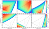 |
Fig. B.1 Same as Fig. 1, but for T = 200 K, p = 1 bar, and N = 0.001. |
| In the text | |
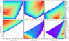 |
Fig. B.2 Same as Fig. 1, but for T = 600 K, p = 1 bar, and N = 0.001. |
| In the text | |
 |
Fig. B.3 Same as Fig. 1, but for T = 400 K, p = 0.01 bar, and N = 0.001. |
| In the text | |
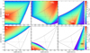 |
Fig. B.4 Same as Fig. 1, but for T = 400 K, p = 100 bar, and N = 0.001. |
| In the text | |
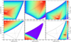 |
Fig. B.5 Same as Fig. 1, T = 400 K, p = 1 bar, and N = 0.001. |
| In the text | |
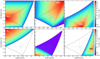 |
Fig. B.6 Same as Fig. 1, but for T = 400 K, p = 1 bar, and N = 0.5. |
| In the text | |
Current usage metrics show cumulative count of Article Views (full-text article views including HTML views, PDF and ePub downloads, according to the available data) and Abstracts Views on Vision4Press platform.
Data correspond to usage on the plateform after 2015. The current usage metrics is available 48-96 hours after online publication and is updated daily on week days.
Initial download of the metrics may take a while.