| Issue |
A&A
Volume 646, February 2021
|
|
|---|---|---|
| Article Number | A131 | |
| Number of page(s) | 19 | |
| Section | Planets and planetary systems | |
| DOI | https://doi.org/10.1051/0004-6361/202038555 | |
| Published online | 19 February 2021 | |
Four Jovian planets around low-luminosity giant stars observed by the EXPRESS and PPPS★,★★
1
European Southern Observatory, Alonso de Córdova 3107,
Vitacura,
Casilla
19001,
Santiago, Chile
e-mail: This email address is being protected from spambots. You need JavaScript enabled to view it.
2
Instituto de Astronomía, Universidad Católica del Norte,
Angamos 0610
1270709,
Antofagasta, Chile
3
University of Southern Queensland, Centre for Astrophysics,
Toowoomba,
QLD 4350, Australia
4
Departamento de Ciencias Físicas Universidad Andrés Bello. Fernández Concha 700,
759-1538,
Las Condes,
Santiago, Chile
5
School of Physics and Astronomy, Queen Mary University,
327 Mile End Road,
London
E1 4NS, UK
6
Instituto de Astrofísica, Facultad de Física, Pontificia Universidad Católica de Chile,
Av. Vicuña Mackenna 4860,
7820436
Macul,
Santiago, Chile
7
Max-Planck-Institut für Astronomie,
Königstuhl 17,
69117
Heidelberg, Germany
8
Departamento de Astronomía, Universidad de Chile,
Camino El Observatorio 1515,
Las Condes,
Santiago, Chile
9
Centro de Astrofísica y Tecnologías Afines (CATA),
Casilla 36-D,
Santiago, Chile
10
Main Astronomical Observatory, National Academy of Sciences of the Ukraine,
03143
Kyiv, Ukraine
11
Facultad de Ingeniería y Ciencias, Universidad Adolfo Ibáñez,
Av. Diagonal las Torres 2640,
Peñalolén,
Santiago, Chile
12
Millennium Institute for Astrophysics,
Santiogo, Chile
13
Instituto de Física y Astronomía, Universidad de Valparaíso,
Casilla 5030,
Valparaíso, Chile
14
Department of Physics and Astronomy, Bucknell University,
Lewisburg,
PA
17837, USA
Received:
1
June
2020
Accepted:
8
December
2020
Abstract
We report the discovery of planetary companions orbiting four low-luminosity giant stars with M⋆ between 1.04 and 1.39 M⊙. All four host stars have been independently observed by the EXoPlanets aRound Evolved StarS (EXPRESS) program and the Pan-Pacific Planet Search (PPPS). The companion signals were revealed by multi-epoch precision radial velocities obtained in nearly a decade. The planetary companions exhibit orbital periods between ~1.2 and 7.1 yr, minimum masses of mpsin i ~ 1.8–3.7 MJ, and eccentricities between 0.08 and 0.42. With these four new systems, we have detected planetary companions to 11 out of the 37 giant stars that are common targets in the EXPRESS and PPPS. After excluding four compact binaries from the common sample, we obtained a fraction of giant planets (mp ≳ 1– 2 MJ) orbiting within 5 AU from their parent star of f = 33.3−7.1+9.0%. This fraction is slightly higher than but consistent at the 1σ level with previous results obtained by different radial velocity surveys. Finally, this value is substantially higher than the fraction predicted by planet formation models of gas giants around stars more massive than the Sun.
Key words: asteroseismology / techniques: radial velocities / planets and satellites: detection / planets and satellites: formation
RV and activity indicator Tables (A.1–A.8) are only available at the CDS via anonymous ftp to cdsarc.u-strasbg.fr (130.79.128.5) or via http://cdsarc.u-strasbg.fr/viz-bin/cat/J/A+A/646/A131
Based on observations collected at La Silla - Paranal Observatory under programs ID’s 085.C-0557, 087.C.0476, 089.C-0524, 090.C- 0345, 096.A-9020(A), 098.A-9019(A) and through the Chilean Telescope Time under programs ID’s CN-12A-073, CN-12B-047, CN-13A-111, CN-2013B-51, CN-2014A-52, CN-15A-48, CN-15B-25 and CN-16A-13.
© ESO 2021
1 Introduction
After the discovery of the first extrasolar planet around a solar-type star (Mayor & Queloz 1995), thousands of new planetary companions have been uncovered. During the 1990s and 2000s, hundreds of them were discovered using the radial velocity (RV) method. More recently, with the advent of dedicated space missions such as Kepler (Borucki et al. 2010) and the Transiting Exoplanet Survey Satellite (TESS; Ricker et al. 2015), the number of newly detected planets has increased by almost an order of magnitude through the exquisite photometric precision achieved by these missions that are capable of measuring transit depths as small as ~200 ppm (e.g., Jenkins et al. 2015). Using this information, we have been able to compute occurrence rates of short-period planets around low-mass M-dwarfs (Mulders et al. 2015; Hardegree-Ullman et al. 2019) and Sun-like stars (Petigura et al. 2013; Barbato et al. 2018). In addition, by combining the transit information with dedicated ground-based RV follow-up, it is possible to fully characterize the physical properties of transiting planetary companions (planet radius, mass, and density; e.g., Jones et al. 2019), allowing us to study their internal structure and composition (e.g., Thorngren et al. 2016). Moreover, long-running RV surveys searching for planetary companions to solar-type stars have provided a detailed understanding of the planet population at short and large orbital separations (e.g., Marcy et al. 2000; Wittenmyer et al. 2020a).
On the other hand, intermediate-mass (IM) stars (M⋆ ≳ 1.5 M⊙) have mainlybeen excluded from long-term RV surveys because it is inherently difficult to measure precision RVs from their optical spectra (e.g., Lagrange et al. 2009), which restricts the amplitudes of the RV signals to the massive companions regime. It is possible, however, to search for planets orbiting such massive stars with precision RVs by studying their post-main-sequence (MS) descendants (e.g., Johnson et al. 2007a). For more than 15 yr different RV surveys have targeted evolved stars, aimed at computing occurrence rates and thus establishing the role of the stellar mass in planetary systems around IM stars (Frink et al. 2001; Setiawan et al. 2003; Sato et al. 2005; Hatzes et al. 2005; Niedzielski et al. 2007; Han et al. 2010; Jones et al. 2011; Wittenmyer et al. 2011). These surveys have detected ≳150 planets and have found interesting correlations between the frequency of giant planets and stellar mass and metallicity (Reffert et al. 2015; Jones et al. 2016; Wittenmyer et al. 2017a). They also discovered a lack of short-period gas giants (Sato et al. 2008; Döllinger et al. 2009).
In this paper we present RV measurements of four giant stars that have been targeted by the EXoPlanets aRound Evolved StarS (EXPRESS; Jones et al. 2011) and the Pan-Pacific Planet Search (PPPS; Wittenmyer et al. 2011). The obtained RVs of these stars revealed periodic variations that are most likely caused by companions in the planetary mass regime. The orbital periods of the planetary companions cover a range from 1.2 to 7.1 yr, and the projected companion masses extend between ~1.8–3.7 MJ. The paper is organized as follows: the observations, data reduction, and RV measurements are presented in Sect. 2. In Sect. 3 we present the host star properties. The RV analysis and orbital fitting is presented in Sect. 4. In Sect. 5 we compute planet detectability curves for all four host stars. In Sect. 6 we study the stellar activity indicators to discard false-positive scenarios, and in Sect. 7 we use the available HIPPARCOS data to search for possible astrometric orbits induced by the companions. Finally, the summary and discussion are presented in Sect. 8.
2 Observations
High-resolution spectra were taken for the four giant stars presented here. These observations were obtained as part of the EXPRESS and PPPS surveys. These two programs share a total of 37 targets, and several planets have been published using their combined data (Jones et al. 2016; Wittenmyer et al. 2016a, 2017a). A description of the observational strategy and data analysis of these two programs is given in the next sections.
2.1 EXPRESS data
In 2009 we began the observing campaign of the EXPRESS targets. The sample consists of a total of 166 bright stars (V < = 8 mag) that can be observed from Chile (Dec < 20 deg). The target selection criteria are explained in Jones et al. (2011). In total, we have obtained ≳15 spectra per star, with a time baseline of ≳5 yr. Based on our observational cadence and on the number of observations, we can efficiently detect planetary companions that induce an RV amplitude of ≳25 m s−1, with orbital periods up to several years. The first EXPRESS observations were performed in 2009 with the fiber echelle (FECH) spectrograph at the 1.5 m telescope, placed in the Cerro Tololo Inter-American Observatory (CTIO). Unfortunately, even though some of these observations were used to detect a few large-amplitude signals (e.g., Jones et al. 2014), most of these observations were discarded because the lack of thermal and mechanical stability and the relatively low resolution of the instrument preclude us from computing RVs with a long-term precision better than ~20–30 m s−1. However, in 2011 the FECH was replaced by an instrument with a much higher resolution that is also more stable, called CHIRON (Tokovinin et al. 2013), which we used until 2016, and then again in 2019. These observations were also complemented since 2010 with the Fiber-fed Extended Range Optical Spectrograph (FEROS; Kaufer et al. 1999). We note that both CHIRON and FEROS observations deliver good-quality data, leading to a long-term precision of ~5–10 m s−1, which is well suited for this program. For the data reduction and Doppler analysis, we developed several automatic tools that have been described extensively in different papers (Jones et al. 2017, 2018), and are briefly described below. The FEROS data are reduced with the CERES code (Brahm et al. 2017), which performs an individual optimal extraction of the echelle orders after applying the detector bias corrections. The orders are traced and extracted using a combined flat-field spectrum that is taken before the start of the science observations. Finally, the wavelength solution is applied to both the science and calibration fiber. Similarly, the CHIRON data are extracted and calibrated using the Yale pipeline (Tokovinin et al. 2013). For the FEROS data, we measured the radial velocities using the cross-correlation technique and the simultaneous calibration method (Baranne et al. 1996). Briefly, we compute the cross-correlation-function (CCF) between a template with a high signal-to-noise ratio (S/N) of the same star. The template is created by stacking all of the FEROS observations for each star after correcting by their relative Doppler shift. To correct for the nightly spectral drift, we subtract the velocity that is measured from the simultaneous calibration lamp, whichis recorded in the coupled-charge device (CCD) by using the simultaneous calibration fiber. This method is repeated independently in four chunks for each of the 25 orders, covering the wavelength range between ~3900–6800 Å (more details can be found Jones et al. 2017). The resulting velocity is computed from the median of 100 individual chunk velocities. The corresponding RV uncertainties are computed from the error in the mean of all 100 chunk velocities. The FEROS RVs and uncertainties are listed in Tables A.1–A.4 (available at the CDS). In addition, the pipeline computes the bisector velocity span (BVS; Queloz et al. 2001), and activity indicators based on the Mount Wilson system (SMW; Duncan et al. 1991), following the method described in Jenkins et al. (2008) and Jones et al. (2017), as well as Hα indexes, following the method presented in Kürster et al. (2003). We note that the internal SMW error bars are inflated by a factor 0.0021, which is added in quadrature. This value corresponds to the standard deviation of the S-index obtained from 34 FEROS spectra of the quiet RV standard star τ Ceti, taken between 2010 and 2017. Similarly, we adopted an internal uncertainty for the Hα indicators of 0.0024.
CHIRON is equipped with an I2 cell, which superimposes a dense absorption spectrum on the stellar light that is recorded in the CCD. To obtain the velocities from the data, we use the I2 cell method, following the prescription presented in Butler et al. (1996), but we use only one Gaussian to model the instrumental profile. We apply this method to ~3 Å chunks in 22 different orders, covering the wavelength range between ~5000 and 6200 Å. The final RVs are obtained from the weighted mean individual chunk velocities. The individual statistical weights are computed from the long-term scatter of each individual chunk velocity. More details can be found in Jones et al. (2017). The CHIRON RVs and uncertainties are listed in CDS Tables A.1–A.4.
Stellar properties.
2.2 PPPS data
The PPPS originated in 2009 as a Southern Hemisphere extension of the established Lick & Keck Observatory survey for planets orbiting northern “retired A stars” (e.g., Johnson et al. 2006, 2007a, 2010). Data from the PPPS have contributed to the discovery of 16 planets, including 8 planets in collaboration with EXPRESS. Notable discoveries include the 3:5 resonant pair of giant planets orbiting HD 33844 (Wittenmyer et al. 2016a) and HD 76920 b, the most eccentric planet ever found to orbit an evolved star (Wittenmyer et al. 2017b; Bergmann et al. 2020). We obtained observationsbetween 2009 and 2015 using the UCLES high-resolution spectrograph (Diego et al. 1990) at the 3.9-meter Anglo-Australian Telescope (AAT). UCLES achieves a resolution of 45 000 with a one-arcsecond slit. An iodine absorption cell provides wavelength calibration from 5000 to 6200 Å. Precise RVs are determined using the iodine-cell technique as noted above and as detailed in Butler et al. (1996). The photon-weighted midtime of each exposure is determined by an exposure meter. All velocities are measured relative to the zeropoint defined by the iodine-free template observation. The UCLES velocities are given in Tables A.1–A.4.
3 Stellar properties
The stellar properties of the studied targets are summarized in Table 1. The BV JHK magnitudes were retrieved from the Tycho-2 catalog (Høg et al. 2000) and the 2-MASS All-Sky catalog (Cutri et al. 2003), and the spectral types from the Michigan Catalog of two-dimensional spectral types for the HD stars (Houk 1978, 1982; Houk & Smith-Moore 1988). The interstellar visual absorption coefficients (AV) were obtained using the dust extinction maps presented in Bovy et al. (2016). The distance to the host stars was computed from the Gaia Data Release 2 (DR2; Gaia Collaboration 2018) parallaxes, after correcting for the systematic offset found by Stassun & Torres (2018). In addition, we recomputed the atmospheric parameters, using an updated version of the code called Spectroscopic Parameters and atmosphEric ChemIstriEs of Stars (SPECIES; Soto & Jenkins 2018; Soto et al. 2020). For this purpose, we used a high S/N template that was built by stacking all of the individual observed FEROS spectra for each star. These new high S/N templates led to internal uncertainties smaller than those presented in Jones et al. (2011). The resulting Teff, log g, and [Fe/H] values are also listed in Table 1. Figure 1 shows the resulting position of the four stars in the Hertzsprung-Russell (HR) diagram. All four host stars first ascend the red giant branch (RGB) phase, and are located in between the RGB base and the luminosity bump. Because no horizontal branch (HB) evolutionary track crosses this region, we can safely identify these stars as first ascending RGB, and thus we can derive their ages in a more accurate way than for clump giants.
Finally, the stellar mass, radius, luminosity, and age of the host stars were estimated using the latest version of the isochrones1 package (Morton 2015). For this, we compared the atmospheric parameters derived with SPECIES to a grid of MESA isochrones and stellar tracks (Dotter 2016) using the MultiNest tool (Feroz et al. 2009; Buchner et al. 2014). Other input quantities are the BV JHK magnitudes and the Gaia DR2 parallax. We note that the new version of SPECIES incorporates the equivalent evolutionary points (EEPs) in the interpolation process (Dotter 2016). This new approach is a key element to properly account for the different speeds at which models with different masses evolve across the HR diagram, and particularly post-MS stars.
The resulting stellar physical parameters are listed in Table 1 and are those adopted for the remaining paper. We note that Soto et al. (2020) validated our method by comparing our results with interferometry, asteroseismology, and spectroscopic results in the literature. This is certainly of great importance, in particular given the controversy about the derived masses of post-MS stars with planets by isochrone interpolation (e.g., Lloyd 2011; Johnson & Wright 2013; Schlaufman & Winn 2013).
The stellar masses presented here are systematically lower than those presented in Jones et al. (2011) by −0.35 M⊙. We also find that the newly computed distances and stellar luminosities are more accurate and in some cases largely depart from those presented in Jones et al. (2011). The main reasons for these departing results are different derived atmospheric parameters, the difference in the Gaia parallaxes compared to the HIPPARCOS ones (van Leeuwen 2007), and different stellar evolutionary tracks and the interpolation schemes used in the two studies.
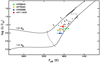 |
Fig. 1 HR diagram showing the position of the four host stars (filled circles). The small black dots represent the 37 targets in common to the EXPRESS and PPPS. The solid lines correspond to 1.0 M⊙ and 1.5 M⊙ PARSEC evolutionary tracks at solar metallicity (Bressan et al. 2012). The dashed line represents the base of the RGB, while the dotted line corresponds to the lower luminosity bump region. |
3.1 Asteroseismology
In addition to the spectroscopic analysis, we performed an asteroseismic analysis of the host stars to derive their physical properties using well-established scaling relations (e.g., Kjeldsen & Bedding 1995; Stello et al. 2017). For this purpose we first analyzed the TESS light curves of all four stars. Unfortunately, all of them were observed only in one sector (~27-day campaigns) in the long-cadence mode (Δt ~ 30 min), which yielded ~1000 individual data-points. This makes detecting the asteroseismic signals very difficult. We found no significant peak in the region of asteroseismic power excess. However, HIP 75092 was also observed by the K2 mission (Howell et al. 2014) in the short-cadence mode (Δt ~ 1 min) in sector 15. The K2 light curve2 contains a total of 129 239 individual measurements collected during 88 days. Before analyzing this data-set, we first corrected the light curve using a linear fit, and we removed outliers using an iterative sigma-clipping rejection algorithm. Using the corrected light curve, we computed a generalized Lomb-Scargle periodogram (GLS; Zechmeister & Kürster 2009) with the astropy.stats Python module to obtain the power spectral density (PSD), from which we can measure the frequency of maximum power (νmax) and the large frequency separation (Δν). After visual inspection of the PSD, we could clearly identify the region of power excess with a high-significance peak around ~180 μHz (see Fig. 2). We thencorrected the background of the PSD in this region using a linear fit, and we convolved the background-corrected PSD with a 7 μHz wide Gaussian kernel. The final νmax value corresponds to the frequency of the maximum of the smoothed PSD. To measure the large frequency separation (Δν), we computed an autocorrelation of the PSD convolved with a narrow 0.1 μHz Gaussian kernel, and we adopted our final Δν from the peak closest to the predicted value from Stello et al. (2009). Using this method, we obtained the following asteroseismic quantities: νmax = 179.69 ± 4.22 μHz and Δν = 14.27 ± 0.01 μHz. The uncertainties correspond to the standard deviation of 1000 bootstrap randomization of the data. Finally, following the scaling relations presented in Stello et al. (2017), we estimated an asteroseismic mass of 1.22 ± 0.09 M⊙ and a radius of 4.77 ± 0.11 R⊙ for HIP 75092. The resulting asteroseismic mass and radius agree well with the spectroscopic values.
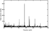 |
Fig. 2 Background-corrected PSD around the asteroseismic power excess region for HIP 75092. |
3.2 Lithium abundance and C12 ∕ C13 isotopic ratio
We computed the lithium (Li) abundance for all four stars using spectral synthesis around the Li doublet at 6708 Å under the assumption of local-thermodynamic-equilibrium (LTE). Briefly, the stellar spectra were fit by a synthetic spectrum that was generated with MOOG (2018 version; Sneden et al. 2012), which accounts for possible blends, and allowing some parameters such as continuum position or the stellar radial velocity to change slightly. For the MOOG input line list, we used a combination of the lists presented in Mélendez et al. (2012) and Carlberg et al. (2012), and we used the ATLAS9 atmospheric models (Castelli & Kurucz 2004). A detailed description of this method will be presented in a forthcoming paper (Aguilera-Gómez et al., in prep.). Unfortunately, we found only upper limits for all four giant stars; they are listed in Table 1.
These upper limits are consistent with expectations of red giants that have already completed their first dredge-up depletion, when the convective envelope of the star deepens at the beginning of the RGB phase (see Fig. 1). Figure 3 shows the Li abundance evolution for these giant stars, calculated using canonical Yale Rotating Evolutionary Code (YREC) models (Pinsonneault et al. 1989). The measured lithium abundance upper limits are overplotted. The resulting upper limits are higher than the theoretical values.
Similarly, we computed the carbon isotopic ratio 12C∕13C, following a similar procedure to that described in Carlberg et al. (2012). We used spectral synthesis to fit the CN bands (both 12C∕N and 13C∕N) in the region between 8000 and 8006 Å. In this spectral region, telluric lines can severely complicate the determination of the ratio. To avoid incorrect measurements, we analyzed all of the available FEROS spectra, and we derived the isotopic ratio only when the telluric lines did not fall near the CN bands. A more detailed description of these measurements will be found in Aguilera-Gómez et al. (in prep.). We report these values in Table 1. In the case of HIP 56640 we could only obtain a lower limit. All carbon isotopic ratios are consistent with first-ascending RGB stars. The carbon isotopic ratio in these stars is expected to decrease from the solar ratio 12C∕13C ~ 90 to 12C∕13C ~ 25. The values foundhere confirm the evolutionary phase of the giants, with no additional mixing in their interiors that would decrease the ratio. Higher values of the carbon isotopic ratio imply a larger error in the measurement because at high ratios, a large difference in 13C only implies verysmall changes in the spectra, thus making it difficult to identify the best fit for the observations. Even small changes to the continuum placement can affect the ratio. However, in spite of the large errors, the carbon isotopic ratio is high and consistent with normal red giant branch stars going through their first dredge-up dilution.
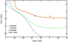 |
Fig. 3 Theoretical lithium abundance evolution from the YREC models for the four giant stars (solid lines). The triangles represent the upper limits to the lithium abundance. |
4 Orbital fitting
To model the RV data and obtain orbital parameters of the companions, we used the Exo-Striker fitting toolbox3 (Trifonov et al. 2019). As a starting point, we performed a frequency analysis of the combined RV time series for each target. The GLS analyses of the available data showed that all four targets contain a very significant periodic RV signal with semiamplitudes well above the RV uncertainties. The period corresponding to the maximum GLS power, phase, and amplitude were used as an initial guess of the parameter optimization process, which aims to determine the best-fit Keplerian orbital parameters of the planetary candidates. With the Exo-Striker we used the Simplex algorithm (Nelder & Mead 1965), which optimizes the negative logarithm of the likelihood function ( ) coupled with a Keplerian model. The optimized parameters are the RV semi-amplitude K, orbital period P, eccentricity e, argument of periastron ω, mean anomalies M for a given epoch (from which we derived the time of periastron passage Tp), and the RV zeropoint offset for each data set. In the case of HIP 90988, we included a linear (
 ) RV trend as an additional fitting parameter. The parameter uncertainties were estimated using an affine-invariant ensemble Markov chain Monte Carlo (MCMC) sampler (Goodman & Weare 2010) in the emcee package (Foreman-Mackey et al. 2013). We adopted noninformative flat priors, and we explored the parameter space starting from the best-fit parameters returned by the Simplex minimization. Depending on the system we studied, we typically ran 100 independent walkers in parallel, in a standard scheme of 1000 burn-in MCMC steps, which we discarded from the analysis, followed by 5000 MCMC steps from which we constructed the parameter posterior distribution. At the end of each MCMC run, we evaluated the sampler acceptance fraction to ensure that the MCMC chains have converged (which should be between 0.2 and 0.5; see Foreman-Mackey et al. 2013). Finally, we adopted the median absolute deviation (MAD) of the MCMC posterior distributions to serve as a 1σ uncertainty estimate of the parameters. We also note that we included the uncertainty in the stellar mass to derive the planet minimum mass and semimajor axis.
We note that before searching for the global minimum, we added in quadrature 7 m s−1 to the RV instrumental errors to account for the excess of RV noise (e.g., Wittenmyer et al. 2016a). We find that this prior jitter level of 7 m s−1 is well justified keeping in mind the known instrumental systematics of FEROS, UCLES, and CHIRON, which are on the same order of magnitude. In addition, evolved stars exhibit short-period p-mode oscillations that contribute to the RV noise. For instance, the scaling relation from Kjeldsen & Bedding (1995) suggest an RV scatter level that agrees well with the adopted RV scatter in this work. As a matter of completeness, however, in our modeling scheme we also optimized the RV jitter for each data set (Baluev 2009). We find that the jitter estimates are very small, often consistent with 0 m s−1, which means that the prior jitter level of 7 m s−1 is indeed adequate. The resulting orbital parameters from our RV analysis and the corresponding uncertainties are listed in Table 2.
4.1 HIP 56640 = HD 100939
We collected a total of 22 FEROS spectra of HIP 56640 and five more UCLES data-points, covering more than 3000 days. These combined data sets revealed a relatively strong RV signal (peak-to-peak variation ~100 m s−1), which is consistent with the presence of a relatively massive (mb sin i = 3.67 ± 0.19 MJ) planetary companion in a long-period orbit (2574.9 ± 86.1 days). Figure 4 shows the FEROS and UCLES RVs and the best Keplerian fit to the data. The orbital parameters are listed in Table 2.
4.2 HIP 75092 = HD 136295
We observed this star in 23 different epochs with FEROS, and we obtained additional 13 UCLES spectra. We computed a GLS periodogram of the combined data sets, and we found a high-significance peak (false-alarm probability ~0.0001) at ~940 days. We complemented these data sets with five new CHIRON observations, which confirmed the RV signal detected in the FEROS and UCLES RVs. These combined data sets span more than ten years of observations. Figure 5 shows the RVs from all three instruments. The best Keplerian fit is overplotted. The periodic RV variation observed in this star is consistent with the Doppler shift induced by a substellar companion with minimum mass of 1.79 ± 0.15 MJ and orbital period of 926.4 ± 12.8 days. With e = 0.42 ± 0.10, this is also the most eccentric of the planets presented here, and one of the most eccentric known planets orbiting giant stars. The resulting orbital parameters are listed in Table 2.
4.3 HIP 90988 = HD 170707
We obtained 25 FEROS, four UCLES, and 13 CHIRON spectra of for HIP 90988. The combined data sets span more than 2700 days. The FEROS and UCLES data revealed a long linear trend, soon after the first several RV measurements were obtained. After collecting additional data, we also realized an ~90 m s−1 peak-to-peak periodic signal that is superimposed on an RV linear trend. Figure 6 shows the RV data of HIP 90988 and the RVsafter subtracting the long-term linear trend. The best-fit Keplerian solution is overplotted. The orbital parameters are listed in Table 2. The observed RV curve is consistent with the presence of a 1.96 ± 0.11 MJ minimum mass planet in a 454-day and low-eccentricity orbit (e = 0.08).
Finally, from the linear trend (dv/dt = –48.99 ± 0.83 m s−1 yr−1) we estimated the minimum mass of the outer companion that is compatible with this value. For this we numerically computed different orbital configurations with increasing orbital period and companion mass, under the assumption of mc ≪ M⋆ and fixing the eccentricity to zero (e.g., Torres 1999). We then imposed that a synthetic curve matches the data when the difference in the observed and simulated RV acceleration term is consistent at the 1σ level and the residuals of the fit are at ~5 m s−1. Here the residuals correspond to the difference between the Keplerian synthetic model and the linear fit to the Keplerian model computed at the time of the observations. We note that a significantly higher value of the residual would be an indication of a quadratic RV term, and it would be present in the real data. Using this method, we obtained the following results: mc sin i ≳ 24 MJ and ac ≳ 9.0 AU. The minimum orbital period of ~23 yr corresponds to about three times the observational time span. The resulting minimum mass of the outer companion is well within the planetary to brown dwarf mass regime. Moreover, the minimum angular separation (~95 mas) is veryclose to inner detection limits for high-contrast imaging, making this system an interesting candidate for further studies to characterize the outer companion (e.g., Ginski et al. 2020) using instruments such as the Spectro-Polarimetric High-contrast Exoplanet REsearch (SPHERE; Beuzit et al. 2019).
Orbital parameters.
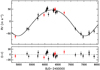 |
Fig. 4 Radial velocity variations of HIP 56640. The black and red dots correspond to FEROS and UCLES velocities, respectively.The best Keplerian solution is overplotted (solid black line). The post-fit residuals are shown in the lower panel. |
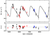 |
Fig. 5 Radial velocity variations of HIP 75092. The black, red and blue dots correspond to FEROS, UCLES and CHIRON velocities, respectively. The best Keplerian solution is overplotted (solid black line). The post-fit residuals are shown in the lower panel. |
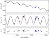 |
Fig. 6 Upper panel: radial velocity variations of HIP 90988. The black, red and blue dots correspond to FEROS, UCLES and CHIRON velocities, respectively. The best Keplerian solution is overplotted (solid black line). Middle panel: RV variations ofHIP 90988 after subtracting a liner trend. Lower panel: post-fit residuals. |
4.4 HIP 114933 = HD 219553
We observed HIP 144933 between August 2009 and November 2017. We collected a total of 19 FEROS, nine UCLES, and 14 CHIRON spectra for this star. The corresponding velocities revealed a long-period periodic variation with an amplitude of ~30 m s−1, most likely induced by a 1.94 ± 0.20 MJ minimum mass planet orbiting at 2.8 AU from the host star. No evidence of a third body in the system is observed for this star. Figure 7 shows the RV variations for all three data sets and the best Keplerian fit. The best-fit orbital elements of HIP 114933 b and their estimated uncertainties are listed in Table 2.
5 Companion detection limits
We computed detection limits for all four stars to assess which planets we are able to detect with these RV data sets. For this, we used the root mean square (RMS) approach, following previous works (e.g., Bowler et al. 2010; Wittenmyer et al. 2020b). Briefly, we computed a large number of synthetic RVs at each observing epoch, corresponding to different companion masses and orbital periods, and zero eccentricity. We then compared the observed RMS of the synthetic data sets to the observed post-fit residuals. We imposed that a system is detected if the RMS of the synthetic RVs is 2.5 times larger than the post-fit residuals RMS of the real data. The results are presented in Fig. 8. The solid lines correspond to 50 and 95% detectability curves. The position of the planetary companions and total observing time span are overplotted. The data are very sensitive (≳95% completeness) to planets with MP ≳ 1.0 MJ and orbital period P ≲ 100 days, or MP ≳ 2.0 mb sin i up to periods of ~1000 days.
6 Stellar activity analysis
To investigate whether stellar phenomena are responsible for the observed RV variations (e.g., Boisse et al. 2011), we analyzed the HIPPARCOS and the All Sky Automated Survey (ASAS; Pojmanski 2002) V -band photometry of all four giant stars in detail. In the analysis we only included HIPPARCOS data with quality flag equal to 0 and 1. Similarly, we only used A- and B-grade ASAS data. For both data sets, we applied a 3 σ clipping filter. We then combined the two data sets after applying a zeropoint offset between them, and we computed a Lomb-Scargle periodogram of the combined data. This procedure not only allowed us to search for long-period signals exceeding their individual total time span, but it also boosted the significance of periodic signals present in the two individual data sets. We found no significant peaks in the periodograms in all four stars.
Similarly, we studied the stellar chromospheric variability using the activity indicators computed by our pipeline (SMW and Hα; see Sect. 2.1) to search for potential periodic signals with periods similar to those attributed to the planetary companions. For this, we computed periodograms of the SMW and Hα activity indexes. We found no significant peak in the region around the expected orbital periods. We also compared these values with the measured RVs. We found a mild correlation between these quantities for HIP 56640 and HIP 75092, mainly explained by a few epochs with values systematically below the mean. To study the significance of this correlation, we also investigated the activity indexes stability with time, using the RV standard stars τ Ceti and HD 72673. We found similar offsets in the SMW values at different epochs, particularly for HD 72673. We interpret these departing values as been caused by instrumental effects (e.g., atmospheric dispersion correction, and blaze function response variability), as noted in Jones et al. (2017), and not due to stellar activity. The HIPPARCOS magnitude (Hp), SMW and Hα indexes variability are summarized in Table 3 for all four stars. For comparison, we also list the values we obtained for τ Ceti (HIP 8102) and HD 72673 (HIP 41926). These stars are photometrically and chromospherically stable. This is expected because they were selected against photometric variability.
Finally, to discard line asymmetry variations as the cause of the observed RVs, we computed FEROS BVS values and repeated the periodogram analysis. Again we found no significant peak in the periodograms. Similarly, we compared the BVSs with the observed radial velocities. In the case of HIP 90988 we first subtracted the RV linear trend. We found a moderate level of correlation in the case of HIP 56640 and HIP 75092. However, as in the case of the activity indicators, we also see systematic offsets in the BVS values at different epochs for the RV standard stars, and in the case of τ Ceti, we observe a positive correlation between the BVS and the SMW values. Moreover, the BVS variability and correlation coefficient between the BVSs and RVs for HD 72673 is higher than the four stars presented here. Therefore we again conclude that the BVS variability observed in the FEROS spectra is dominated by intrinsic instrumental variation with time. The resulting BVS, SMW, and Hα values are listed in Tables A.5–A.8.
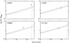 |
Fig. 8 Detection limits for all 4 host stars. The solid lines correspond to 50 and 95% detection efficiency (from bottom to top). Theblack dots show the position of the companion. The vertical dashed lines corresponds to the total RV time coverage. |
Stellar activity indicators.
7 HIPPARCOS astrometry
To rule out that the RV signals are induced by low-inclination binary companions, we attempted to measure the orbital inclination angles using the combined HIPPARCOS astrometric data and the available RV measurements, following the procedure described in Sahlmann et al. (2011) and Jones et al. (2017). Using this method, we derived inclination angles for three of the binary companions detected by the EXPRESS program (Jones et al., in prep.). In this particular case, we could not detect the astrometric signal induced by the companion. Based on the planet-to-star mass ratio, the astrometric amplitude signals are expected to be ≲0.1 mas, which is well below the HIPPARCOS precision. Moreover, in all four cases, the Gaia DR2 astrometric excess noiseis equal to zero, meaning that there is no indication of an astrometric motion induced by a companion. When we assume edge-on orbits, the astrometric signals for four six stars is at the ~20–30 μarcsec level, which is comparable to the Gaia detection limit.
Finally, we compared the HIPPARCOS and Gaia DR2 parameters (parallax, pmRA, and pmDEC). The differences in these quantities are presented in Fig. 9. The values from the two catalogs are consistent, except for HIP 90988, where the difference in pmRA is beyond 3σ. This departure is expected because of the outer companion detected in the RVs.
8 Discussion
8.1 Summary
We presented precision radial velocities of four giant stars that have been targeted for about a decade by the EXPRESS and PPPS radial velocity surveys. The radial velocities were computed from spectroscopic data collected with three different instruments mounted on 1- to 3-meter class telescopes in the Southern Hemisphere. The RV data have revealed periodic signals that are most likely explained by the presence of substellar companions. From the Keplerian fits we derived companion minimum masses between ~1.8 and 3.7 MJ, orbital periods of 1.2–7.1 yr and eccentricities between 0.08 and 0.42. Additionally, HIP 90988 presents a long-term RV trend of −49.0 m s−1 yr−1, which is most likely induced by an outer body with a minimum mass in the planetary mass regime (mc sin i ≳ 24 MJ). We note that either further RV follow-up or high-contrast imaging observations are needed to confirm or discard the planetary nature of the companion.
From our combined photometric and spectroscopic analysis, we found that all four host stars are low-luminosity giants with masses between 1.04 and 1.39 M⊙. Based on their position on the HR diagram, these stars can be unambiguously identified as first-ascending RGB stars, and they have completed their first dredge-up (see Fig. 1).
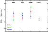 |
Fig. 9 Difference in the Gaia and HIPPARCOS catalog parameters for all four stars. The red, green, and blue points correspond to the difference in parallax, pmRA, and pmDEC. Here pmRA corresponds to μ cos(Dec), where μ = dRA∕dt. |
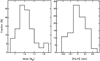 |
Fig. 10 Mass and metallicity distribution of the 37 targets in common to the EXPRESS and PPPS. |
8.2 Occurrence rate from the targets in common to EXPRESS and PPPS
Figure 1 shows the position in the HR diagram for all the 37 stars in common to the EXPRESS and PPPS. Similarly, Fig. 10 shows their stellar mass and metallicity distribution, derived with the newest version of the SPECIES code (see Sect. 3). The median mass and metallicity of this sample is 1.21 ± 0.16 M⊙ and 0.0 ± 0.1 dex, respectively. Interestingly, 10 out of the 37 stars have been identified as spectroscopic binaries, and 4 of them are in a compact system (a ≲ 5.0 AU; Bluhm et al. 2016), where the formation and survival of circumprimary (s-type) giant planets is fully suppressed (see Moe & Kratter 2019 and references therein). For each star, we collected ≳20 individual spectra between 2009 and 2019. For the planet candidate host stars we have taken additional spectra, typically ≳40 RV epochs in total. This combined data set allowed us to efficiently detect giant planets (mb sin i ≳ 1–2 MJ) orbiting their parent parent star up to an orbital distance of ~5 AU (see Fig. 8). With the results presented here, we have found a total of 13 giant planets around 11 stars within 5 AU, including two multiple systems (Jones et al. 2015a,b; Wittenmyer et al. 2016a). Figure 11 shows the semimajor axis distribution versus the stellar mass for all 13 planets detected around the 37 stars. The position of the two unpublished planet candidates is also shown. The orbital distribution is substantially different than for giant planets orbiting solar-type stars, and it is distinctively characterized by a desert of close-in planets (a ≲ 0.5 AU) and a complete absence of hot Jupiters (Sato et al. 2008; Döllinger et al. 2009), which are known to be rare (f = 0.49 ± 0.28%) around low-luminosity RGB stars (Grunblatt et al. 2019). We note that the innermost planet (a ~ 0.4 AU) in this sample is found in a multiple system. Considering the high mass ratio between the inner and outer planets (q ~ 5), we might speculate that the presence of the outer companion has played an important role in the orbital configuration of the system. However, the mechanism is not clear, particularly considering that more massive planets can destabilize the orbits of smaller planets (Ida et al. 2013). When we exclude from the analysis the four compact binaries, we obtain a fraction of giant stars hosting at least one Jovian planet within 5 AU of  . We note that we did not apply any completeness correction to account for potential missing planets. The lower and upper error bars correspond to the 1σ equal-tailed confidence limit, following the Bayesian approach presented in Cameron (2011). By restricting the orbital distance to 2.5 and 3.0 AU, we obtained a fraction of
  and
and  , respectively. The first value is significantly higher than the 4.2 ± 0.7 and 8.9 ± 2.9% fraction of Jovian planets within 2.5 AU for solar-type stars and higher mass subgiants reported by Johnson et al. (2007b). However, our results are compatible at the 1σ level with
  within 3 AU obtained by Bowler et al. (2010) from a uniform sample of intermediate-mass subgiants. In addition, Reffert et al. (2015) studied the occurrence rate of gas giants orbiting giant stars targeted by the Lick Survey (Frink et al. 2001) as a function of the stellar mass and metallicity. In the mass bin between 1.0 and 1.8 M⊙ stars, they found a fraction of
  , for [Fe/H] between −0.12 and +0.04, and
  for [Fe/H] between +0.04 and +0.20 dex. The median mass and metallicity of the 11 host stars in common to the PPPS and EXPRESS sample is 1.29 ± 0.20 M⊙ and 0.06 ± 0.11 dex, respectively. This means that the host stars are significantly more massive than the Sun, which probably explains the striking differences in the fraction and orbital distribution when compared to planets orbiting solar-type stars, which is discussed in the next section.
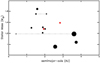 |
Fig. 11 Semimajor axis distribution vs. the mass of the host star for the planets in common to the EXPRESS and PPPS. The filled black circles correspond to the confirmed and published planets, and the filled red circles correspond to the unpublishedplanet candidates. The symbol size is proportional to the minimum mass of the planet. The dotted lines connect the position of the inner and outer planets in multiple systems. |
8.3 Detection fraction and orbital distribution in the context of the core-accretion model
There are two main ingredients for the formation of giant planets in the core-accretion model: the dust and gas content in the protoplanetary disk. A high surface density of dust (σd) is needed torapidly form planetesimals before the depletion of the dusty component in the disk (≲3–6 Myr; e.g., Haisch et al. 2001). They will subsequently form protoplanet cores by coagulation and subsequent runaway and oligarchic growth (e.g., Kokuba & Ida 1998). In the inner region of the disk, σd might not be high enough to form massive cores, but beyond the snow line, this value is predicted to increase by a factor ~3–4, leading to protoplanets that are about five times more massive (Kennedy & Kenyon 2008). After reaching a mass of ≳5–10 M⊕, these cores can efficiently accrete the surrounding gas in the disk (e.g., Pollack et al. 1996), eventually becoming a gas giant planet. During the gas accretion process onto the protoplanetary core, a significant amount of gas (and a correspondingly high gas surface density; σg), must be present in the disk before gas dissipation by accretion in the central star (Muzerolle et al. 2005) and photoevaporation (Kennedy & Kenyon 2009). Having these formation processes in mind, we can understand, at least in a qualitative way, the observed properties of gas giants in the EXPRESS and PPPS common sample as follows. The host stars are slightly metal rich (median metallicity of +0.06 ± 0.04 dex), ensuring a relatively high σd to efficientlyform relatively massive protoplanets. Similarly, because the disk mass scales with the stellar mass (e.g., Andrews et al. 2013), both σd and σg are enhanced compared to lower mass stars (e.g., Laughlin et al. 2004), and thus the minimum core mass to undergo runaway gas accretion can be quickly formed in a wide range of orbital separation (Ida & Lin 2005). These protoplanetary cores will then efficiently accrete gas from the disk, resulting in a high fraction of giant planets. Theoretical models predict an increase in the giant planets fraction with the stellar mass from ~1% at 0.4 M⊙, to ~10% at 1.5 M⊙ (Kennedy & Kenyon 2008). However, we found a substantially higher fraction of gas giants at ~1.3 M⊙, meaning that their formation efficiency might be higher than predicted.
Finally, the larger orbital separation observed for gas giants orbiting intermediate-mass stars when compared to solar-type host stars (Johnson et al. 2007a) might be explained by the effect of the stellar mass on the disk properties and evolution. In particular, not only can massive enough cores be formed at wider orbital separations, but the position of the snow line also moves outward as a result of the increasing stellar luminosity with increasing mass. In these two cases, in situ formation either inside or beyond the snow line occur at larger a. Similarly, because of the increasing accretion and photoevaporation rates with increasing stellar mass (Muzerolle et al. 2005; Burkert & Ida 2007), the inner part of the disk is also more rapidly depleted (e.g., Currie et al. 2007). As a result and because of the shorter disk lifetime, type II migration (Papaloizou & Lin 1984) might be rapidly halted, preventing giant planets from moving inward, which would explain the relatively large orbital distance and the lack of hot Jupiters orbiting evolved intermediate-mass stars, as is the case of the planets presented here (Ribas et al. 2015). On the other hand, the absence of short-period planets might partially be due to planet engulfment even before the host star leaves the MS (Hamer & Schlaufman 2019). However, theoretical calculations show that low-luminosity giant stars are not expected to efficiently engulf planet orbiting beyond ~0.1 AU (e.g., Villaver & Livio 2009; Kunitomo et al. 2011; Villaver et al. 2014). This is supported observationally by the discovery of transiting short-period giant planets around evolved stars (e.g., Lillo-box et al. 2014; Grunblatt et al. 2017; Jones et al. 2017).
Acknowledgements
We acknowledge the traditional owners of the land on which the AAT stands, the Gamilaraay people, and pay our respects to elders past and present. C.A.G. acknowledges support from the National Agency for Research and Development (ANID) FONDECYT Postdoctoral Fellowship 2018 Project 3180668. J.S.J. acknowledges support by FONDECYT grant 1201371, and partial support from CONICYT project Basal AFB-170002. M.R.D. is supported by CONICYT-PFCHA/Doctorado Nacional- 21140646, Chile.
Appendix A Radial velocity tables
Radial velocities for HIP 56640.
Radial velocities for HIP 75092.
 |
Fig. A.1 Correlation between the orbital parameters derived by the Exo-Striker analysis for HIP 56640. |
 |
Fig. A.2 Correlation between the orbital parameters derived by the Exo-Striker analysis for HIP 75092. |
 |
Fig. A.3 Correlation between the orbital parameters derived by the Exo-Striker analysis for HIP 90988. |
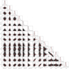 |
Fig. A.4 Correlation between the orbital parameters derived by the Exo-Striker analysis for HIP 114933. |
Radial velocities for HIP 90988.
Radial velocities for HIP 114933.
FEROS BVS, SMW, and Hα values for HIP 56640.
FEROS BVS, SMW, and Hα values for HIP 75092.
FEROS BVS, SMW, and Hα values for HIP 90988.
FEROS BVS, SMW, and Hα values for HIP 114933.
References
- Andrews, S. M., Rosenfeld, K. A., Kraus, A. L., & Wilner, D. 2013, ApJ, 771, 129 [NASA ADS] [CrossRef] [Google Scholar]
- Baluev, R. V. 2009, MNRAS, 393, 969 [NASA ADS] [CrossRef] [Google Scholar]
- Baranne, A., Queloz, D., Mayor, M., et al. 1996, A&A, 119, 373 [Google Scholar]
- Barbato, D., Bonomo, A. S., Sozzetti, A., & Morbidelli, R. 2018, ArXiv eprints [arXiv:1811.08249] [Google Scholar]
- Bergmann, C., Jones, M. I., Zhao, J., et al. 2020, PASA, accepted [Google Scholar]
- Beuzit, J. L., Vigan, A, Mouillet, D., et al. 2019, A&A, 631, A155 [NASA ADS] [CrossRef] [EDP Sciences] [Google Scholar]
- Bluhm, P., Jones, M. I., Vanzi, L., et al. 2016, A&A, 593, A133 [NASA ADS] [CrossRef] [EDP Sciences] [Google Scholar]
- Boisse, I., Bouchy, F., Hebrard, G., et al. 2011, A&A, 528, A4 [NASA ADS] [CrossRef] [EDP Sciences] [Google Scholar]
- Borucki, W. J., Koch, D., Basri, G., et al. 2010, Science, 327, 977 [NASA ADS] [CrossRef] [PubMed] [Google Scholar]
- Bovy, J., Rix, H.-W., Green, G. M., Schlafly, E. F., & Finkbeiner, D. P. 2016, ApJ, 818, 130 [NASA ADS] [CrossRef] [Google Scholar]
- Bowler, B. P., Johnson, J. A., Marcy, G. W., et al. 2010, ApJ, 709, 396 [NASA ADS] [CrossRef] [Google Scholar]
- Brahm, R., Jordán, A., & Espinoza, N. 2016, PASP, 129, 34002 [Google Scholar]
- Bressan, A., Marigo, P., Girardi, L., et al. 2012, MNRAS, 427, 127 [NASA ADS] [CrossRef] [Google Scholar]
- Buchner, J., Georgakakis, A., Nandra, K., et al. 2014, A&A, 564, A125 [NASA ADS] [CrossRef] [EDP Sciences] [Google Scholar]
- Burkert, A., & Ida, S. 2007, ApJ, 660, 845 [NASA ADS] [CrossRef] [Google Scholar]
- Butler, R. P., Marcy, G. W., Williams, E., et al. 1996, PASP, 108, 500 [NASA ADS] [CrossRef] [Google Scholar]
- Cameron, E. 2011, PASA, 28, 128 [NASA ADS] [CrossRef] [Google Scholar]
- Castelli, F., & Kurucz, R. L. 2004, ArXiv e-prints [arXiv:astro-ph/0405087v1] [Google Scholar]
- Carlberg, J. K., Cunha, K., Smith, V., & Majewski, S. R. 2012, ApJ, 757, 109 [NASA ADS] [CrossRef] [Google Scholar]
- Currie, T., Balog, Z., Kenyon, S. J., et al. 2007, ApJ, 659, 599 [NASA ADS] [CrossRef] [Google Scholar]
- Cutri, R. M., Skrutskie, M. F., van Dyk, S., et al. 2003, VizieR Online Data Catalog: II/246 [Google Scholar]
- Diego, F., Charalambous, A., Fish, A. C., & Walker, D. D. 1990, Proc. SPIE, 1235, 562 [NASA ADS] [CrossRef] [Google Scholar]
- Dohlen, K., Langlois, M., Saisse, M., et al. 2008, SPIE Conf. Ser., 7014, 70143L [Google Scholar]
- Döllinger, M. P., Hatzes, A. P., Pasquini, L., Guenther, E. W., & Hartmann, M. 2009, A&A 505, 1311 [NASA ADS] [CrossRef] [EDP Sciences] [Google Scholar]
- Dotter, A. 2016, ApJS, 222, 8 [NASA ADS] [CrossRef] [Google Scholar]
- Duncan, D. K., Vaughan, A. H., Wilson, O. C., et al. 1991, ApJS, 76, 383 [NASA ADS] [CrossRef] [Google Scholar]
- Feroz, F., Hobson, M. P., & Bridges, M. 2009, MNRAS, 398, 1601 [NASA ADS] [CrossRef] [Google Scholar]
- Foreman-Mackey, D., Hogg, D. W., Lang, D., & Goodman, J. 2013, PASP, 125, 306 [Google Scholar]
- Frink, S., Quirrenbach, A., Fischer, D., Röser, S., & Schilbach, E. 2001, PASP, 113, 173 [NASA ADS] [CrossRef] [Google Scholar]
- Gaia Collaboration (Brown, A. G. A., et al.) 2018, A&A, 616, A10 [NASA ADS] [CrossRef] [EDP Sciences] [Google Scholar]
- Ginski, C., Mugrauer, M., Adam, C., Vogt, N., & van Holstein, R. 2021, A&A, accepted https://doi.org/10.1051/0004-6361/201838964 [Google Scholar]
- Goodman, J., & Weare, J. 2010, Commun. Appl. Math. Comput. Sci., 5, 65 [Google Scholar]
- Grunblatt, S. K., Huber, D., Gaidos, E., et al. 2017, AJ, 154, 254 [NASA ADS] [CrossRef] [Google Scholar]
- Grunblatt, S. K., Huber, D., Gaidos, E., et al. 2019, AJ, 158, 227 [NASA ADS] [CrossRef] [Google Scholar]
- Haisch, E. Jr., Lada, E. A., & Lada, C. J. 2001, ApJ, 553, 153 [Google Scholar]
- Hamer, J. H., & Schlaufman, K. C. 2019, AJ, 158, 190 [Google Scholar]
- Han, I., Lee, B. C., Kim, K. M., et al. 2010, A&A, 509, A24 [NASA ADS] [CrossRef] [EDP Sciences] [Google Scholar]
- Hardegree-Ullman, K. K., Cushing, M. C., Muirhead, P. S., & Christiansen, J. L. 2019, AJ, 158, 75 [NASA ADS] [CrossRef] [Google Scholar]
- Hatzes, A. P., Guenther, E. W., Endl, M., et al. 2005, A&A, 437, 743 [NASA ADS] [CrossRef] [EDP Sciences] [Google Scholar]
- Høg, E., Fabricius, C., Makarov, V., et al. 2000, A&A, 355, 27 [Google Scholar]
- Houk, N. 1982, Michigan Catalogue of Two-dimensional Spectral Types for the HD Stars, 2, Declinations −40.0° to −26.0° (Department of Astronomy, University of Michigan, Ann Arbor, MI) [Google Scholar]
- Houk, N., & Smith-Moore, M. 1978, Michigan Catalogue of Two-dimensional Spectral Types for the HD Stars, 2, Declinations −53.0° to −40.0° (Department of Astronomy, University of Michigan, Ann Arbor, MI) [Google Scholar]
- Houk, N., & Smith-Moore, M. 1988, Michigan Catalogue of Two-dimensional Spectral Types for the HD Stars, 4, Declinations −26.0° to −12.0° (Department of Astronomy, University of Michigan, Ann Arbor, MI) [Google Scholar]
- Howell, S. B., Sobeck, C., Haas, M., et al. 2014, PASP, 126, 398 [NASA ADS] [CrossRef] [Google Scholar]
- Ida, S., & Lin,D. N. C. 2005, ApJ, 626, 1045 [Google Scholar]
- Ida, S., Lin, D. N. C., & Nagasawa, M. 2013, ApJ, 775, 42 [NASA ADS] [CrossRef] [Google Scholar]
- Jenkins, J. S., Jones, H. R. A., Pavlenko, Y., et al. 2008, A&A, 485, 571 [NASA ADS] [CrossRef] [EDP Sciences] [Google Scholar]
- Jenkins, J. M., Twicken, J., D., Batalha, N. M., et al. 2015, ApJ, 150, 56 [Google Scholar]
- Johnson, J. A., & Wright, J. T. 2013, ArXiv eprints [arXiv:1307.3441] [Google Scholar]
- Johnson, J. A., Marcy, G. W., Fischer, D. A., et al. 2006, ApJ, 652, 1724 [NASA ADS] [CrossRef] [Google Scholar]
- Johnson, J. A., Fischer, D. A., Marcy, G. W., et al. 2007a, ApJ, 665, 785 [NASA ADS] [CrossRef] [Google Scholar]
- Johnson, J. A., Butler, R. P., Marcy, G. W., et al. 2007b, ApJ, 670, 833 [NASA ADS] [CrossRef] [Google Scholar]
- Johnson, J. A., Aller, K. M., Howard, A. W., & Crepp, J. R. 2010, PASP, 122, 905 [NASA ADS] [CrossRef] [Google Scholar]
- Jones, M. I., Jenkins, J. S., Rojo, P., & Melo, C. H. F. 2011, A&A, 536, A71 [NASA ADS] [CrossRef] [EDP Sciences] [Google Scholar]
- Jones, M. I., Jenkins, J. S., Bluhm, P., Rojo, P., & Melo, C. H. F. 2014, A&A, 566, A113 [NASA ADS] [CrossRef] [EDP Sciences] [Google Scholar]
- Jones, M. I., Jenkins, J. S., Rojo, P., Melo, C. H. F., & Bluhm, P. 2015a, A&A, 573, A3 [NASA ADS] [CrossRef] [EDP Sciences] [Google Scholar]
- Jones, M. I., Jenkins, J. S., Rojo, P., Olivares, F., & Melo, C. H. F. 2015b, A&A, 580, A14 [NASA ADS] [CrossRef] [EDP Sciences] [Google Scholar]
- Jones, M. I., Jenkins, J. S., Brahm, R., et al. 2016, A&A, 590, A38 [NASA ADS] [CrossRef] [EDP Sciences] [Google Scholar]
- Jones, M. I., Brahm, R., Wittenmyer, R. A., et al. 2017, A&A, 602, A58 [NASA ADS] [CrossRef] [EDP Sciences] [Google Scholar]
- Jones, M. I., Brahm, R., Espinoza, N., et al. 2018, A&A, 613, A76 [CrossRef] [EDP Sciences] [Google Scholar]
- Jones, M. I., Brahm, R., Espinoza, N., et al. 2019, A&A, 625, A16 [NASA ADS] [CrossRef] [EDP Sciences] [Google Scholar]
- Kaufer, A., Stahl, O., Tubbesing, S., et al. 1999, The Messenger 95, 8 [Google Scholar]
- Kennedy, G. M., & Kenyon, S. J. 2008, ApJ, 673, 502 [NASA ADS] [CrossRef] [Google Scholar]
- Kennedy, G. M., & Kenyon, S. J. 2009, ApJ, 695, 1210 [NASA ADS] [CrossRef] [Google Scholar]
- Kjeldsen, H., & Bedding, T. R. 1995, A&A, 293, 87 [NASA ADS] [Google Scholar]
- Kokubo, E., & Ida, S. 1998, Icarus, 131, 171 [Google Scholar]
- Kunitomo, M., Ikoma, M., Sato, B., et al. 2011, ApJ, 737, 66 [NASA ADS] [CrossRef] [Google Scholar]
- Kürster, M., Endl, M., Rouesnel, F., et al. 2003, A&A, 403, 1077 [NASA ADS] [CrossRef] [EDP Sciences] [Google Scholar]
- Laughlin, G., Bodenheimer, P., & Adams, F. C. 2004, ApJ, 612, L73 [NASA ADS] [CrossRef] [Google Scholar]
- Lagrange, A.-M., Desort, M., Galland, F., Udry, S., & Mayor, M. 2009, A&A, 495, 335 [NASA ADS] [CrossRef] [EDP Sciences] [Google Scholar]
- Lillo-Box, J., Barrado, D., Moya, A., et al. 2014, A&A, 562, A109 [NASA ADS] [CrossRef] [EDP Sciences] [Google Scholar]
- Lloyd, J. P. 2011, ApJ, 739, 49 [NASA ADS] [CrossRef] [Google Scholar]
- Marcy, G., Butler, R. P., Fischer, D. A., & Vogt, S. S. 2016, ASPC, 213, 85 [Google Scholar]
- Mawet, D., Milli, J., Wahhaj, Z., et al. 2014, ApJ, 792, 97 [NASA ADS] [CrossRef] [Google Scholar]
- Mayor, M., & Queloz, D. 1995, Nature, 378, 355 [Google Scholar]
- Meléndez, J., Bergemann, M., Cohen, J. G., et al. 2012, A&A, 543, A29 [NASA ADS] [CrossRef] [EDP Sciences] [Google Scholar]
- Meschiari, S., Wolf, A. S., Rivera, E., et al. 2009, PASJ, 121, 1016 [Google Scholar]
- Moe, M., & Kratter, K. 2019, MNRAS, submitted [arXiv:1912.01699] [Google Scholar]
- Morton, T. D. 2015, Astrophys. Source Code Libr. [record ascl:1503.010] [Google Scholar]
- Mulders, G. D., Pascucci, I., & Apai, D. 2015, ApJ, 814, 130 [NASA ADS] [CrossRef] [Google Scholar]
- Muzerolle, J., Luhman, K. L., Briceño, C., Hartmann, L., & Calvet, N. 2005, ApJ, 625, 906 [NASA ADS] [CrossRef] [Google Scholar]
- Nelder, J. A., & Mead, R. 1965, Comput. J., 7, 308 [CrossRef] [Google Scholar]
- Niedzielski, A., Konacki, M., Wolszczan, A., et al. 2007, ApJ, 669, 1354 [NASA ADS] [CrossRef] [Google Scholar]
- Papaloizou, J., & Lin, D. N. C. 1984, ApJ, 285, 818 [NASA ADS] [CrossRef] [Google Scholar]
- Petigura, E. A., Howard, A. W., & Marcy, G. W. 2013, PNAS, 110, 19273 [NASA ADS] [CrossRef] [Google Scholar]
- Pinsonneault, M. H., Kawaler, S. D., Sofia, S., & Demarque, P. 1989, ApJ, 338, 424 [NASA ADS] [CrossRef] [Google Scholar]
- Pojmanski, G. 2002, Acta Astron., 52, 397 [NASA ADS] [Google Scholar]
- Pollack, J. B., Hubickyj, O., Bodenheimer, P., et al. 1996, Icarus, 124, 62 [NASA ADS] [CrossRef] [Google Scholar]
- Queloz, D., Henry, G. W., Sivan, J. P., et al. 2001, A&A, 379, 279 [NASA ADS] [CrossRef] [EDP Sciences] [Google Scholar]
- Reffert, S., Bergmann, C., Quirrenbach, A., Trifonov, T., & Künstler, A. 2015, A&A 574, A116 [NASA ADS] [CrossRef] [EDP Sciences] [Google Scholar]
- Ribas, A., Bouy, H., & Merín, B. 2015, A&A, 576, A52 [NASA ADS] [CrossRef] [EDP Sciences] [Google Scholar]
- Ricker, G. R., Winn, J. N., Vanderspek, R., et al. 2015, J. Astron. Teles., Instrum. Syst., 1, 014003 [Google Scholar]
- Sahlmann, J., Ségransan, D., Queloz, D., et al. 2011, A&A, 525, A95 [NASA ADS] [CrossRef] [EDP Sciences] [Google Scholar]
- Sato, B., Kambe, E., Takeda, Y., et al. 2005, PASJ, 57, 97 [Google Scholar]
- Sato, B., Toyota, E., Omiya, M., et al. 2008, PASJ, 60, 1317 [NASA ADS] [Google Scholar]
- Scargle, J. D. 1982, ApJ, 263, 835 [Google Scholar]
- Schlaufman, K. C., & Winn, J. N. 2013, ApJ, 772, 143 [NASA ADS] [CrossRef] [Google Scholar]
- Setiawan, J., Pasquini, L., da Silva, L., von der Lühe, O., & Hatzes, A. 2003, A&A, 397, 1151 [NASA ADS] [CrossRef] [EDP Sciences] [Google Scholar]
- Sneden, C., Bean, J., Ivans, I., et al. 2012, Astrophys. Source Code Libr. [record ascl:1202.009] [Google Scholar]
- Soto, M., & Jenkins, J. S. 2018, A&A, 615, A76 [NASA ADS] [CrossRef] [EDP Sciences] [Google Scholar]
- Soto, M., Jones, M. I., & Jenkins, J. S. 2020, A&A, submitted https://doi.org/10.1051/0004-6361/202039357 [Google Scholar]
- Stassun, K. G., & Torres, G. 2018, ApJ, 862, 61 [Google Scholar]
- Stello, D., Chaplin, W. J., Basu, S., Elsworth, Y., & Bedding, T. R. 2009, MNRAS, 400, 80 [Google Scholar]
- Stello, D., Huber, D., Grundahl, F., et al. 2017, MNRAS, 472, 4110 [NASA ADS] [CrossRef] [Google Scholar]
- Tokovinin, A., Fischer, D. A., Bonati, M., et al. 2013, PASP, 125, 1336 [NASA ADS] [CrossRef] [Google Scholar]
- Thorngren, D. P., Fortney, J. J., Murray-Clay, R. A., & Lopez, E. D. 2016, ApJ, 831, 64 [NASA ADS] [CrossRef] [Google Scholar]
- Torres, G. 1999, PASP, 111, 169 [NASA ADS] [CrossRef] [Google Scholar]
- Trifonov, T., 2019, Astrophys. Source Code Libr., [record ascl:1906.004] [Google Scholar]
- van Leeuwen, F. 2007, A&A, 474, 653 [NASA ADS] [CrossRef] [EDP Sciences] [Google Scholar]
- Villaver, E., & Livio, M. 2009, ApJ, 705, 81 [Google Scholar]
- Villaver, E., Livio, M., Mustill, A. J., & Siess, L. 2014, ApJ, 794, 3 [NASA ADS] [CrossRef] [Google Scholar]
- Winn, J. N., Johnson, J. A., Albrecht, S., et al. 2009, ApJ, L99, 103 [Google Scholar]
- Wittenmyer, R. A., Endl, M., Wang, L., et al. 2011, ApJ, 743, 184 [NASA ADS] [CrossRef] [Google Scholar]
- Wittenmyer, R. A., Johnson, J. A., Butler, R. P., et al. 2016a, ApJ, 818, 35 [NASA ADS] [CrossRef] [Google Scholar]
- Wittenmyer, R. A., Liu, F., Wang, L., et al. 2016b, AJ, 152, 19 [NASA ADS] [CrossRef] [Google Scholar]
- Wittenmyer, R. A., Jones, M. I., Zhao, J., et al. 2017a, AJ, 153, 51 [NASA ADS] [CrossRef] [Google Scholar]
- Wittenmyer, R. A., Jones, M. I., Horner, J., et al. 2017b, AJ, 154, 274 [NASA ADS] [CrossRef] [Google Scholar]
- Wittenmyer, R. A., Wang, S., Horner, J., et al. 2020a, MNRAS, 492, 377 [CrossRef] [Google Scholar]
- Wittenmyer, R. A., Butler, R. P., Horner, J., et al. 2020b, MNRAS, 491, 5248 [CrossRef] [Google Scholar]
- Zechmeister, M., & Kürster, M. 2009, A&A, 496, 577 [NASA ADS] [CrossRef] [EDP Sciences] [Google Scholar]
The corrected K2 project team light curve was retrieved from the MAST portal: https://mast.stsci.edu/portal/Mashup/Clients/Mast/Portal.html
All Tables
All Figures
|
Fig. 1 HR diagram showing the position of the four host stars (filled circles). The small black dots represent the 37 targets in common to the EXPRESS and PPPS. The solid lines correspond to 1.0 M⊙ and 1.5 M⊙ PARSEC evolutionary tracks at solar metallicity (Bressan et al. 2012). The dashed line represents the base of the RGB, while the dotted line corresponds to the lower luminosity bump region. |
| In the text | |
|
Fig. 2 Background-corrected PSD around the asteroseismic power excess region for HIP 75092. |
| In the text | |
|
Fig. 3 Theoretical lithium abundance evolution from the YREC models for the four giant stars (solid lines). The triangles represent the upper limits to the lithium abundance. |
| In the text | |
|
Fig. 4 Radial velocity variations of HIP 56640. The black and red dots correspond to FEROS and UCLES velocities, respectively.The best Keplerian solution is overplotted (solid black line). The post-fit residuals are shown in the lower panel. |
| In the text | |
|
Fig. 5 Radial velocity variations of HIP 75092. The black, red and blue dots correspond to FEROS, UCLES and CHIRON velocities, respectively. The best Keplerian solution is overplotted (solid black line). The post-fit residuals are shown in the lower panel. |
| In the text | |
|
Fig. 6 Upper panel: radial velocity variations of HIP 90988. The black, red and blue dots correspond to FEROS, UCLES and CHIRON velocities, respectively. The best Keplerian solution is overplotted (solid black line). Middle panel: RV variations ofHIP 90988 after subtracting a liner trend. Lower panel: post-fit residuals. |
| In the text | |
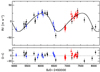 |
Fig. 7 Same as Fig. 5 for HIP114933. |
| In the text | |
|
Fig. 8 Detection limits for all 4 host stars. The solid lines correspond to 50 and 95% detection efficiency (from bottom to top). Theblack dots show the position of the companion. The vertical dashed lines corresponds to the total RV time coverage. |
| In the text | |
|
Fig. 9 Difference in the Gaia and HIPPARCOS catalog parameters for all four stars. The red, green, and blue points correspond to the difference in parallax, pmRA, and pmDEC. Here pmRA corresponds to μ cos(Dec), where μ = dRA∕dt. |
| In the text | |
|
Fig. 10 Mass and metallicity distribution of the 37 targets in common to the EXPRESS and PPPS. |
| In the text | |
|
Fig. 11 Semimajor axis distribution vs. the mass of the host star for the planets in common to the EXPRESS and PPPS. The filled black circles correspond to the confirmed and published planets, and the filled red circles correspond to the unpublishedplanet candidates. The symbol size is proportional to the minimum mass of the planet. The dotted lines connect the position of the inner and outer planets in multiple systems. |
| In the text | |
|
Fig. A.1 Correlation between the orbital parameters derived by the Exo-Striker analysis for HIP 56640. |
| In the text | |
|
Fig. A.2 Correlation between the orbital parameters derived by the Exo-Striker analysis for HIP 75092. |
| In the text | |
|
Fig. A.3 Correlation between the orbital parameters derived by the Exo-Striker analysis for HIP 90988. |
| In the text | |
|
Fig. A.4 Correlation between the orbital parameters derived by the Exo-Striker analysis for HIP 114933. |
| In the text | |
Current usage metrics show cumulative count of Article Views (full-text article views including HTML views, PDF and ePub downloads, according to the available data) and Abstracts Views on Vision4Press platform.
Data correspond to usage on the plateform after 2015. The current usage metrics is available 48-96 hours after online publication and is updated daily on week days.
Initial download of the metrics may take a while.