| Issue |
A&A
Volume 646, February 2021
|
|
|---|---|---|
| Article Number | A100 | |
| Number of page(s) | 11 | |
| Section | Numerical methods and codes | |
| DOI | https://doi.org/10.1051/0004-6361/202038552 | |
| Published online | 15 February 2021 | |
Learning to do multiframe wavefront sensing unsupervised: Applications to blind deconvolution
1
Instituto de Astrofísica de Canarias, 38205 La Laguna, Tenerife, Spain
e-mail: aasensio@iac.es
2
Departamento de Astrofísica, Universidad de La Laguna, 38205 La Laguna, Tenerife, Spain
3
Max Planck Institute for Solar System Research, Justus-von-Liebig-Weg 3, 37077 Göttingen, Germany
Received:
1
June
2020
Accepted:
18
December
2020
Context. Observations from ground-based telescopes are severely perturbed by the presence of the Earth’s atmosphere. The use of adaptive optics techniques has allowed us to partly overcome this limitation. However, image-selection or post-facto image-reconstruction methods applied to bursts of short-exposure images are routinely needed to reach the diffraction limit. Deep learning has recently been proposed as an efficient way to accelerate these image reconstructions. Currently, these deep neural networks are trained with supervision, meaning that either standard deconvolution algorithms need to be applied a priori or complex simulations of the solar magneto-convection need to be carried out to generate the training sets.
Aims. Our aim here is to propose a general unsupervised training scheme that allows multiframe blind deconvolution deep learning systems to be trained with observations only. The approach can be applied for the correction of point-like as well as extended objects.
Methods. Leveraging the linear image formation theory and a probabilistic approach to the blind deconvolution problem produces a physically motivated loss function. Optimization of this loss function allows end-to-end training of a machine learning model composed of three neural networks.
Results. As examples, we apply this procedure to the deconvolution of stellar data from the FastCam instrument and to solar extended data from the Swedish Solar Telescope. The analysis demonstrates that the proposed neural model can be successfully trained without supervision using observations only. It provides estimations of the instantaneous wavefronts, from which a corrected image can be found using standard deconvolution techniques. The network model is roughly three orders of magnitude faster than applying standard deconvolution based on optimization and shows potential to be used on real-time at the telescope.
Key words: stars: imaging / methods: data analysis / techniques: image processing
© ESO 2021
1. Introduction
The observation of astronomical objects from ground-based observatories is degraded by the presence of turbulence in the Earth’s atmosphere. One obvious solution is to move the observatory to space to avoid the atmosphere, but this is often not feasible due to technological or budgetary reasons. Additionally, the largest and most advanced telescopes are always built on the ground, because they usually require state-of-the-art technology.
Active and, especially, adaptive optics (AO), that is, deformable optics that can compensate for the effect of the atmosphere almost in real time, have facilitated the use of ground-based telescopes. The combination of very fast sensors (that allow the measurement of instantaneous wavefront) and deformable mirrors (that correct the wavefront that reaches the science cameras) can produce images very close to the diffraction limit of the telescopes, at least in a reduced field of view (FOV). As a demonstration of the importance of AO, currently more than 25% of the observations in some large-aperture telescopes like Keck and VLT use an AO device (Rigaut 2015), and this figure reaches ∼100% in the case of solar observations. These AO systems have been extremely successful in the near-infrared, where the perturbing effect of the atmosphere is less important. AO systems working for visible and near-ultraviolet wavelengths are much more demanding and, although lagging behind, much effort is currently going into making them robust. Successful use of AO systems in the visible has been demonstrated by the field of solar physics, where such systems are commonly used in telescopes like the Swedish 1 m Solar Telescope (SST) at the Observatorio del Roque de los Muchachos (Spain), the GREGOR telescope on the Observatorio del Teide (Spain), or the Goode Solar Telecope (GST) on the Big Bear Observatory (USA).
Even if AO systems are working properly, some residual wavefront perturbations are still present on the images. These residuals are a consequence of the accumulation of different sources, such as for example (i) imperfect measurement of the wavefront by wavefront sensors (WFSs), (ii) imperfect correction of this wavefront measurement by the deformable mirrors, (iii) some delay between the measurement and the actuation, (iv) static aberrations in the telescope+instrument optics that are not corrected by AO systems, and (v) poor correction of the FOV away from the optical axis (classical AO systems with one WFS and one pupil deformable mirror produce their best correction close to this axis).
For the above reasons, reaching the diffraction limit of a telescope in a large FOV is not often possible without a posteriori image-correction methods. The simplest techniques of a posteriori correction are based on frame selection, also known as lucky imaging. These methods rely on the fact that the wavefront deformation due to the atmosphere is small at some selected frames when a long burst of short-exposure images is acquired. The fraction of such lucky frames decreases when the atmospheric turbulence increases. Another problem with this technique lies in its low photon efficiency, because a very large fraction of the frames are discarded. An additional drawback is that it only works properly for small or medium-sized telescopes, with diameters below 2.5 m. In larger telescopes, the probability that low turbulence is found in a significant fraction of the telescope aperture quickly goes to zero. Instruments like FastCam (Oscoz et al. 2008), which we use in this paper, are fully based on the exploitation of this idea.
More elaborate techniques are based on speckle methods (Labeyrie 1970; von der Lühe 1993), which make use of all the recorded frames to get an estimation of the image. Paxman et al. (1992) later proposed some improvements, which are now at the base of many of the most advanced methods currently in use. The first improvement was the assumption of a very flexible parametric point spread function (PSF) that is especially suited for telescopic observations. This is done via a linear expansion of the aberrations in the pupil of the system in a suitable basis. Although other options have also been explored (e.g., Markham & Conchello 1999), the approach proposed by Paxman et al. (1992) is very efficient. The second was the use of phase-diversity techniques (Gonsalves & Chidlaw 1979), which consist of simultaneously taking pairs of images (or more) with a known static differential aberration. The third improvement was a proper treatment of the noise models, which result in different optimizations. Löfdahl & Scharmer (1994) and Löfdahl et al. (1998), based on the work of Paxman et al. (1992), applied this latter technique to solar observations, while Löfdahl et al. (2002) extended it to the multiframe case. van Noort et al. (2005) later applied it to the multiobject and multiframe case, developing the successful multi-object multi-frame blind deconvolution (MOMFBD) code, which is systematically applied in solar filtergraph observations. Hirsch et al. (2011) also considered an online version of multiframe blind deconvolution that is much more memory efficient.
All previous approaches are conveniently based on the maximization of a proper likelihood function that is automatically defined by the statistical properties of the noise. As maximum likelihood methods can be sensitive to noise, Bayesian approaches are also widespread in the blind deconvolution community (see, e.g., Molina et al. 2001, and references therein). This approach, in which a priori information about the object or the PSF is put forward, are arguably more important in single-frame deconvolution (e.g., Blanco & Mugnier 2011), but they can also be applied to the multiframe case. For instance, Bucci et al. (1999) regularize the phase-diversity problem by imposing additional constraints on the merit function, while Blanc et al. (2003) consider the marginal deconvolution in the same problem. Along this line, Thelen et al. (1999) solve the blind deconvolution problem by assuming a multivariate Gaussian prior for the wavefront parameters.
The emergence of deep learning has revolutionized the field of image processing. In particular, methods have been proposed for the deblurring of video sequences (Wieschollek et al. 2017), for the rapid estimation of PSFs from images (Möckl et al. 2019), and for the modeling of simple PSFs (Herbel et al. 2018) for large-scale surveys. It is evident that methods that make use of many frames to produce a single deconvolved frame make much better use of the collected photons and should always be preferred over lucky imaging techniques. However, their main disadvantage resides in the large computational requirements, especially when applied to long rapid bursts of large images, as in solar observations. Supercomputers become necessary to deconvolve the data and deep learning can be a remedy to lower the computational requirements. With this idea in mind, Asensio Ramos et al. (2018) recently developed an extremely fast multiframe blind deconvolution approach based on supervised deep learning. Although the model is general, the results were only considered for solar observations. It makes use of a fully convolutional deep neural network that was trained, whilst supervised, with images previously corrected with the help of MOMFBD. Once trained, this method can deconvolve bursts of short-exposure 1k × 1k images in ∼5 ms with an appropriate Graphical Processing Unit (GPU). This opens up the possibility, for instance, of doing image deconvolution on the fly at the telescope.
Although a step forward in terms of speed, the neural approach developed by Asensio Ramos et al. (2018) has two main issues. The first one is that it is trained with supervision, so one needs to use the MOMFBD algorithm to build the training set. Though not a major obstacle, a method that does not need this previous step would be preferable. The second issue is that the method developed by Asensio Ramos et al. (2018) outputs only the deconvolved images. No estimation of the wavefront in each individual frame is produced. Estimating the wavefronts can be helpful to check the performance of the telescope and instrument in order to understand the performance of the AO or to reuse them when there are several instruments pointing to the same FOV. For these reasons, in this work we present a new deep learning scheme that can be trained in a fully unsupervised manner whilst also producing an estimation of the wavefront for each observed frame. Given the lack of supervision, the method can be generally applied to any type of object, either point-like or extended, once a sufficient number of observed images is available.
2. Unsupervised training
2.1. Image formation
In this paper, we follow the formalism used by Löfdahl et al. (2002) and van Noort et al. (2005), based on the work of Paxman et al. (1992). The deconvolution of a burst of short-exposure images1 is possible once the linear physics of image formation is imposed. Let us assume that o is the image of the object under study outside the Earth’s atmosphere. We acquire a burst of N images taken at times {t1, t2, …, tN} through a linear space invariant instrument (in our case, telescope+instrument) and corrupted with uncorrelated Gaussian noise (see Sect. 2.3 for more details). Therefore, the image ij at time tj that is sensed at the detector is given by:

where is the convolution operator, sj is the PSF of the atmosphere at time tj, nj is the uncorrelated Gaussian noise component, and r is the spatial coordinate on the image. We note that the object o(r) is common to all the N images. Any blind deconvolution method then tries to simultaneously recover both o(r) and s = {s1, …, sN} from the burst of images i = {i1, …, iN}. We note that the index j can also be used to refer to simultaneous images containing known differential aberrations following the prescriptions of phase-diversity.
The convolution operation in Eq. (1) can be translated into simple multiplications if we transform the equation to the Fourier space:

where the uppercase symbols represent the Fourier transform of the lowercase symbols and u represents Fourier frequencies. The symbol Sj(u) is known as the optical transfer function (OTF). The noise is still uncorrelated and Gaussian thanks to the linear character of the Fourier transform.
The space invariant approximation is often violated in normal conditions because of the presence of high-altitude turbulence in the atmosphere. This produces different PSFs for different portions of the FOV, with sizes defined by the anisoplanatic angle. For this reason, when deconvolving an extended object, spatially variant PSFs need to be considered. We note that the overlap-add (OPA) approach is routinely used in solar physics with the MOMFBD code with excellent results (e.g., van Noort et al. 2005). However, more precise approaches like the widespread method of Nagy & O’Leary (1998) and the recent space-variant OLA (Hirsch et al. 2010) methods can be used (see Denis et al. 2015, for a review).
2.2. Description of point spread functions
The OTF can be written in terms of the generalized pupil function:
![$$ \begin{aligned} S_j(u) = \mathcal{F} \left[ |\mathcal{F} ^{-1}(P_j) |^2 \right]. \end{aligned} $$](/articles/aa/full_html/2021/02/aa38552-20/aa38552-20-eq3.gif)
In other words, the OTF is the Fourier transform of the PSF, which in turn is given by the autocorrelation of the generalized pupil function. The generalized pupil function can be written as:

where Aj describes the amplitude modulation of the pupil (the aperture of the telescope, including the primary and secondary and any existing spider) and ϕj describes the phase at the pupil (also known as wavefront). A flat wavefront produces an Airy diffraction PSF. The presence of atmospheric turbulence affects this phase by introducing a nonflat wavefront, which, as a consequence, generates a complex PSF. We note that this formalism allows us to take into account a phase-diversity channel by writing down the generalized pupil function as:

where Δ is the added diversity, which is usually a defocus.
Following Paxman et al. (1992), we assume that the wavefront can be written (in radians) as a linear combination on a suitable basis. The Zernike functions (e.g., Noll 1976) are among the most useful functions for reproducing functions in the circle because they are orthogonal in the unit circle. Despite their useful mathematical properties, Zernike functions are not especially suited to efficiently reproducing wavefronts produced by atmospheric turbulence. This is because the covariance matrix of the coefficients of the Zernike modes under Kolmogorov turbulence (also termed Noll covariance matrix) is nondiagonal. Specifically, the elements of the Noll covariance matrix are given by (Roddier 1990)
where
where Γ(x) is the Gamma function (Abramowitz & Stegun 1972), and D and r0 are the diameter of the telescope and Fried radius, respectively. The δmi, mj Kronecker-like symbol is strictly zero when mi ≠ mj or when i − j is odd (unless mi = mj = 0) and one otherwise.
As a consequence, we use in this paper the so-called Karhunen-Loeve (KL) modes (e.g., van Noort et al. 2005), which are obtained by numerically diagonalizing the covariance matrix given by Eq. (6). This diagonalization is carried out using the singular value decomposition, ordering the modes by their singular value. Therefore, the wavefront is finally written as:
where M is the number of functions used in the linear combination, (x, y) refer to coordinates in the pupil plane, αji are the ith KL coefficient of the j-th wavefront and KLi(x, y) are obtained as linear combinations of the Zernike functions.
2.3. Loss function
From a Bayesian point of view, the multiframe blind deconvolution problem requires the computation of the joint posterior distribution for the object o and the α = {α1, α2, …, αN} coefficients, conditioned on the observations:

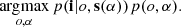
where the vector s(α) refers to the PSFs obtained with the coefficients α. The posterior distribution is the product of the likelihood, p(i|o, s(α)), and the prior, p(o, α). We highlight the fact that the likelihood depends on α through the PSFs. Sampling the full high-dimensional posterior is computationally impracticable and so point estimates are almost always used. The maximum a posteriori (MAP) solution is therefore given by:
Much success has been obtained following this path when dealing with single-image blind deconvolution (e.g., Molina et al. 2001; Mugnier et al. 2004; Blanco & Mugnier 2011; Babacan et al. 2012; Farrens et al. 2017; Fétick et al. 2020).
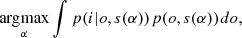
The MAP solution introduces some regularization but it does not exploit the full potential of the Bayesian approach. Methods based on a Type-II maximum-likelihood approach require solving the following optimization problems in marginalized posteriors:
These arguably lead to better results (see, e.g., Blanco & Mugnier 2011; Fétick et al. 2020) and we defer their consideration in the neural unsupervised approach to a future publication.
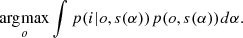
In this paper, we follow the approach of Löfdahl & Scharmer (1994), Paxman et al. (1996), and van Noort et al. (2005) and consider all objects and wavefront coefficients to be equally probable a priori. Taking negative logarithms, the maximum likelihood solution that we seek is:
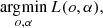
where L(o, α) = − log p(i|o, s(α)) is the negative log-likelihood, often termed ‘loss function’ in the machine learning literature. To simplify the notation, we drop the dependency of the log-likelihood on the PSF and show directly its dependence on the wavefront coefficients.
2.3.1. Stationary Gaussian-noise model
Under the assumption of uncorrelated, independent, and identically distributed additive Gaussian noise, one can write the loss function as:
![$$ \begin{aligned} L(o,{\boldsymbol{\alpha }}) = \sum _r \sum _{j=1}^N \gamma _j \left[ i_j(r) - o(r) * s_j(r;{\boldsymbol{\alpha }}) \right]^2, \end{aligned} $$](/articles/aa/full_html/2021/02/aa38552-20/aa38552-20-eq15.gif)
where the summation is carried out for all positions r (obviously now discretized in pixels) of all the images taken at times {t1, t2, …, tN}. The term γj is an estimation of the inverse noise variance of the jth image. Applying both Parseval’s and the convolution theorems, one can write down the log-likelihood with the Fourier components (dropping unimportant constants):
with the summation now carried out over Fourier frequencies. Given the historical success of the approach of Paxman et al. (1996), we utilize a frequency filter Hj to minimize the effect of noise in the observed images. The maximum likelihood solution is then formally given by
This loss function is nonconvex in the set of parameters {O, α}, and one can apply an alternating optimization method to solve it. This scheme iteratively considers the two following subproblems:
The solution to the linear least squares problem of Eq. (18) is (Paxman et al. 1992):
where the caret indicates an estimated quantity. The filter H(u) is used to ensure that all spatial frequencies for which all OTFs are zero are not used and its specific form is discussed in Sect. 2.3.3.
Another possibility that we explore is to remove the filter from the loss function (16) and instead use a Gaussian prior for the object (although it is known that such priors generate overly smooth images; see Tipping & Bishop 2002). The resulting estimation of the object is a Wiener filter (e.g., Blanco & Mugnier 2011):
where Sn is the power spectral density (PSD) of the noise and S0(u) is an estimation of the PSD of the object. The simplest possible Wiener filter assumes Sn/S0(u) = K, with K a constant.
This estimated object can then be inserted back into Eq. (16) resulting in a loss function that does not depend on the object (see, e.g., Paxman et al. 1992; van Noort et al. 2005). For the estimation of the object of Eq. (20) we have
![$$ \begin{aligned} L({\boldsymbol{\alpha }})=\sum _u H(u) \left[ \sum _{j} \gamma _j \left|I_{j}(u)\right|^{2}- \frac{\left|\sum _{j} \gamma _j I_{j}^{*}(u) S_{j}(u;{\boldsymbol{\alpha }})\right|^{2}}{\sum _{j} \gamma _j \left|S_{j}(u;{\boldsymbol{\alpha }})\right|^{2}} \right]. \end{aligned} $$](/articles/aa/full_html/2021/02/aa38552-20/aa38552-20-eq22.gif)
For the Wiener filter estimation of the object, we end up with:
![$$ \begin{aligned} L({\boldsymbol{\alpha }})=\sum _u \left[ \frac{\mathcal{S} ({\boldsymbol{\alpha }}) \sum _{j} \gamma _j \left|I_{j}(u)\right|^{2}-\left|\sum _{j} \gamma _j I_{j}^{*}(u) S_{j}(u;{\boldsymbol{\alpha }})\right|^{2}}{\mathcal{S} ({\boldsymbol{\alpha }}) + \frac{S_n}{S_0(u)} } \right], \end{aligned} $$](/articles/aa/full_html/2021/02/aa38552-20/aa38552-20-eq23.gif)
where
In case many objects are observed simultaneously so that they share the same wavefront, the total loss function is the result of summing the loss function computed for each one of the objects.
Equations (22) and (23) define loss functions that can be optimized with respect to α to find the instantaneous wavefront. From these coefficients, the PSFs affecting each one of the N frames of the burst can be computed. Once the wavefronts are computed, the deconvolved image can easily be obtained using Eqs. (20) or (21), although more elaborate nonblind deconvolution solutions can also be used. We use Eq. (20) for all the results shown in this paper, so that:
![$$ \begin{aligned} O = P_{+} \left[ \mathcal{F} ^{-1}(\hat{O}(u)) \right], \end{aligned} $$](/articles/aa/full_html/2021/02/aa38552-20/aa38552-20-eq25.gif)
where we also enforce non-negativity by using the P+ operator, which sets all negative pixels to zero.
2.3.2. Other noise models
The dominant noise in astronomical imaging is photon noise, which follows a Poisson distribution. The main difficulty in using the Poisson log-likelihood in our scheme is that a closed form solution to Eq. (18) has not been found yet (Paxman et al. 1992). Fortunately, the Gaussian distribution is a good approximation to the Poissonian once the number of photons is larger than about 20. For this to happen, one has to make the distribution nonstationary with a variance equal to the number of photons, which avoids an easy transformation to the Fourier space.
In any case, the observations that we use for training are not in the low-photon limit and the sources are not very bright with respect to the background. As a consequence, and because our objective is to show how a neural network can be trained unsupervised for performing multiframe blind deconvolution, we only refer to the Gaussian case with constant γj per frame.
2.3.3. Filter
The visual appearance of the deconvolved image heavily depends on the specific details of the nonblind deconvolution technique that we use once the wavefront coefficients are obtained. The results shown in this paper were computed using Eq. (20), with the filter proposed by Löfdahl & Scharmer (1994) that has shown very good practical results in solar images (Löfdahl et al. 2002; van Noort et al. 2005). The filter has the following form:
where we set all values below 0.2 and above 1 to zero. Finally, we remove all isolated peaks in the filter that cannot be directly connected to the peak at zero frequency with H > 0.2.
2.4. Data preprocessing
In addition to the standard ill-defined multiframe blind deconvolution problem, which can be alleviated with prior information, this method is always subject to some fundamental ambiguities that are harder to deal with (Paxman et al. 2019). One of the most critical in our approach is the fact that the global tip-tilt cannot be obtained. If the object is shifted by a certain amount, one can always compensate for this with a tip-tilt contribution in the wavefront so that the image of the object remains stationary. Consequently, any learning method that we use will become confused about the specific amount of tip-tilt to infer from the images. We force the results to have small tip-tilt coefficients by pre-aligning all images of the burst so that the object of interest is, on average, centered on the FOV. We do this by computing the sum of all the images in the burst, computing the peak emission and shifting this peak to lie at the center of the image with pixel precision.
2.5. Neural architecture
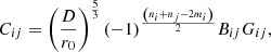
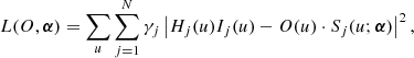
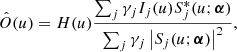
Our neural approach is based on the construction of a neural network that can directly predict the vector α from the images of the burst. This architecture is broadly made of the following components. The first is a convolutional neural network shared for all frames of the burst that extracts features from individual images of size W × W. Two recurrent neural networks (RNNs) follow and they take into account the time evolution of the tip-tilt and high-order coefficients. The RNN in charge of the tip-tilt is not applied to the first frame, which is assumed to have zero tip-tilt. The main purpose of this RNN is to give the relative tip-tilt with respect to the first frame. The high-order RNN is applied to all frames. Two fully connected neural networks (FCLO and FCHO) are shared by all frames and produce two heads for the prediction of tip-tilt and high-order aberrations. The two predictions are concatenated and, finally, we find a layer that computes the OTFs from the wavefront coefficients, which are then plugged into the loss function of Eq. (22) for training the architecture end-to-end. Our approach is graphically depicted in Fig. 1 and in the following we describe each component in detail.
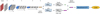 |
Fig. 1. Block diagrams showing the architecture of the network and how it is trained unsupervisedly. The details of each layer are specified in Table 1 and in Sect. 2.5. |
2.5.1. Convolutional neural network
The aim of the first element of the architecture is to summarize the images and extract all relevant information in a vector that can be used later for the prediction of the wavefront coefficients. This component is shared among all frames, so that it can be applied in parallel for all the inputs images. This neural network is a fully convolutional encoder whose properties are summarized in Table 1. The first step is a convolutional layer with a 3 × 3 kernel that generates 32 channels from the input tensor. Both in the application to point-like objects and to extended objects, we consider an input tensor with several channels. These are outlined explicitly in Sects. 3 and 4. Then, a series of standard convolutional blocks made from the consecutive application of batch normalization (Ioffe & Szegedy 2015), an exponential linear unit activation function (ELU; Clevert et al. 2015), and a convolutional layer with the kernel size specified in Table 1 are applied, generating intermediate feature tensors. In order to accelerate convergence, skip connections are added between the initial layer of a block and the last one. This final layer, indicated in orange, uses a kernel of size W/8 × W/8 to produce a vector of size 512 as output. We note that the input images need to have a size multiple of 23 to produce an integer number of latent features.
Architecture of the encoder–decoder network.
2.5.2. Recurrent neural network
The aim of the RNNs is to estimate the tip-tilt and high-order coefficients of the wavefront for all images of the burst while keeping some memory from the rest of the frames. The RNNs can exploit any existing temporal correlation, which is a consequence of the rapid cadence of the observations. Additionally, it can potentially take into account that all frames share the same object, which can be helpful for a better estimation of the aberrations.
Although it is not possible to detect an absolute tip-tilt for a single image, we can use the first frame as a reference and estimate the tip-tilt of all remaining frames relative to the first one. Both RNNs are gated recurrent units (GRU; Cho et al. 2014), which are able to deal with relatively long sequences. We have also experimented with long-term short memory units (Hochreiter & Schmidhuber 1997) with good results, although they are more computationally demanding. Gated recurrent units contain an internal state (cell) that remembers values over long sequences, and gates (reset and update) that are used to control the flow of information into and out of the cell. We choose the cell to be a vector of length 512, of the same length as the input. We also choose the GRU to be bidirectional, so it attends to the inputs in the two possible directions, from frame 1 to frame N and vice versa.
2.5.3. Fully connected neural networks
Two fully connected neural networks produce the final estimation of the tip-tilt and high-order aberrations. The layers are defined by the consecutive application of two linear transformations of sizes 512 × 512 and 512 × 512, each one followed by an ELU activation. The two heads are obtained by predicting the tip-tilt with a final linear transformation of size 512 × 2 and the remaining high-order aberrations with a linear transformation of size 512 × (M − 2). The predicted wavefront coefficients are computed by applying a final activation function atanh(bx). After some trial-and-error, we found that a = 2 and b = 1/10 gave good results. As the output is limited to the interval [ − a, a], one can increase a if very large aberrations are expected.
2.5.4. Computation of OTFs
Once the wavefront coefficients are known for all images in the burst, one can use Eq. (9) to compute the phase on the pupil. Then, the generalized pupil function is obtained from Eq. (4) and the OTF from Eq. (3). This, together with the Fourier transforms of the input images, are all the ingredients needed for the computation of the loss function using Eq. (22).
2.6. Training
Training is done by modifying the parameters of the neural networks so that the loss function of Eq. (22) is minimized for a suitable training set. The several components of our architecture have a total number of ∼7.7 M free parameters. Training is carried out using backpropagation, that is, computing the derivative of the loss function with respect to the free parameters and using this gradient to modify them. The recurrent neural network needs to be trained using backpropagation in time. To this end, it is unrolled for 25 steps and considered as a normal fully connected neural network.
3. Results for point-like objects
As a first step, we consider point-like objects. These are not really the main subject of deconvolution methods because their properties (e.g., astrometry) can be measured with other methods (e.g., Weigelt 1977). However, they can be useful to verify whether or not the estimated wavefronts are representative of the instantaneous PSFs.
3.1. Baseline
In order to verify the ability of our neural approach to correctly estimate the wavefront coefficients, we compare them with a standard multiframe blind deconvolution method. This baseline is obtained by minimizing the loss function of Eq. (22) using the KL coefficients of the wavefront in each frame as unknowns. We use PyTorch to optimize this loss function using the Adam optimizer with a learning rate of 0.1. This learning rate was selected by trial and error. The average computing time per iteration for the deconvolution of 100 frames is ∼0.8 s. The typical number of iterations for convergence is around 70, so the deconvolution can be achieved in around one minute. Obtaining reliable results for sources with reduced signal-to-noise ratios (S/Ns) per frame turned out to be challenging and, on some occasions, impossible.
3.2. Training set
For the examples shown in this section we choose observations carried out with the FastCam instrument mounted on the Nordic Optical Telescope (NOT) on the Observatorio del Roque de los Muchachos (La Palma, Spain). FastCam is a lucky imaging instrument jointly developed by the Spanish Instituto de Astrofísica de Canarias and the Universidad Politécnica de Cartagena. The instrument uses an Andor iXon DU-897 back-illuminated EMCCD containing a 512 × 512 pixel frame. The observations were carried out with a standard I Johnson-Bessel filter at an effective wavelength of 824 nm with a width of 175 nm. The pixel size was 0.0303″. The telescope diameter is 2.56 m, with a central obscuration of 0.51 m, giving a diffraction limit of 0.0786″. The observations were obtained on four consecutive nights on 2007 October 3–6, and include the following objects: GJ1002, GJ144, GJ205, GJ661, RHY1, and RHY44, for a total of several hundred thousand images of 128 × 128 pixels during the four-day run. Some of these objects are single stars in the FOV and others contain a pair of stars. The training set consists of 40 bursts of 1000 images each with an exposure time of 30 ms, enough to efficiently freeze the atmospheric turbulence. The images are taken at different times, and they cover reasonably variable seeing conditions. A validation set of nine bursts, not used for training, was captured and set aside to check for overfitting. Given the unsupervised nature of our approach, the neural network can be easily refined by adding more observations which can cover different seeing conditions.
The training is done by randomly extracting 1000 short bursts of 25 frames (this is the number of unrolled steps of the GRU recurrent component of our architecture) from each one of the 40 available observations, for a total of 40 000 training examples. To facilitate the training, the images are normalized by computing the maximum and minimum in the burst and mapping these values to the [0, 1] interval. Additionally, we use two channels as input, one containing the normalized image itself, which can be useful for inferring properties of the center of the PSF, and another one containing its square root, which gives a better contrast to the tails of the PSF. Once the wavefront coefficients are computed, this normalization is not needed and the deconvolved image can be reconstructed using the original images.
The following augmenting strategy is applied to help improve the generalization capabilities of the neural network. Each burst is randomly rotated 0, 90, 180, or 270 degrees and flipped horizontally or vertically with equal probability. The neural networks are implemented in PyTorch 1.6 (Paszke et al. 2019). We use the Adam optimizer (Kingma & Ba 2014), with a learning rate of 3 × 10⁻⁴ and a batch size of 16, during 25 epochs. We found that the chosen learning rate produces suitable results and it was kept fixed for all experiments. As a consequence of the serial nature of the recurrent network, each epoch takes roughly 17 min, so the total training time is roughly 7 h on a single NVIDIA RTX 2080 Ti GPU. A large fraction of the computing time in the forward pass occurs on the computation of the OTFs and the computation of the loss function.
When in evaluation mode, the outputs of the network are the wavefront coefficients. Unless one is interested in computing the deconvolved image, the calculation of the OTF can be safely ignored. Perhaps the largest difference with respect to the direct optimization of the loss function is that the computing time for a single pass for 100 frames is 20 ms, almost 3000 times faster. This time includes the input and output time to and from the GPU, respectively, and contains some overheads that can be easily avoided. Additionally, thanks to the inherent parallelization in GPUs, the time per deconvolution can be reduced if several stars are deconvolved concurrently. The only limitation is the amount of memory on the GPU.
3.3. Point spread functions
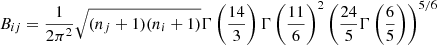
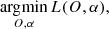
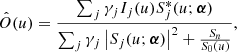
Figure 2 shows examples of the inferred PSFs for different stars from the test set. We show the fir st five frames of the burst in the upper row. We can immediately verify that the seeing conditions and S/N are different in all the examples we consider. For instance, the spread of the images in σ-Ori is much larger than that of GJ661, indicating greater turbulence.
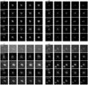 |
Fig. 2. Original frames of the burst (first row), estimated PSF with the neural approach (second row) and the baseline (fourth row), together with the reconstructed individual images (third and fifth rows). Several sources with different seeing conditions and characteristics are displayed. |
The second row of the panels displays the instantaneous PSF (we display the square root to increase the dynamic range of the plot) estimated by the neural approach, while the fourth row shows the results of the baseline. The results clearly show that, in general, we are capturing the shape of the PSF correctly, including a large fraction of the wings. After extensive experiments, we have not found any clear sign of PSF degeneracy, which is fundamentally a consequence of assuming a pupil-based PSF.
Finally, as a consistency check, we re-convolve the image obtained from Eq. (20) with the estimated PSF in both the neural and baseline cases. Our aim with this experiment is to give a visual approximate cross-check of the quality of the inferred PSF. Obviously, the resulting images should be similar to each observed frame, apart from the obvious noise reduction consequence of the cleaner deconvolved image. However, one should be cautious because the result strongly depends on the quality of the deconvolved image, which crucially depends on the filter in the case of Eq. (20) or the estimated PSD of the object in the case of Eq. (21). In any case, one can see minute details of the image that are reproduced with great fidelity in the re-convolved image. Perhaps one could argue that, in cases of very bad seeing with complex PSFs as in the case of σ-Ori, the re-convolved object is slightly more diffuse than the original one. However, the neural approach captures enough details of the PSF so that the ensuing deconvolved image can be made of very high quality.
3.4. Karhunen-Loeve coefficients
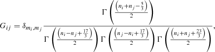
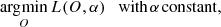
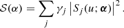
A different way of comparing the baseline and our neural approach is by analyzing the inferred wavefront coefficients. Figure 3 shows the first 36 KL modes for σ-Ori: the baseline in blue and those obtained with the neural network in orange. These results are relevant because the results of the baseline have been used by (van Noort 2017) to correct strictly simultaneous spectropolarimetric data with excellent results. Consequently, our approach can produce fundamentally the same instantaneous PSFs with a much reduced computational burden. Apart from that, it turns out to be relatively trivial to obtain instantaneous properties of the PSF (e.g., Strehl ratio) from these coefficients.
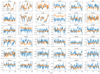 |
Fig. 3. Time evolution of the first 36 coefficients of the phase in the KL basis in radians for the σ-Ori observation. The parameters found by the classical MFBD solution are shown in blue, while those inferred by the neural network are shown in orange. |
The tip-tilt coefficients (first and second coefficients) are very well estimated. The same happens with KL8 and KL9. There are some discrepancies in some of them, especially in KL10. In general, we find that the high-order coefficients are correctly obtained on average, but their amplitude is short in comparison with those of the baseline. In any case, there are potential quasi-ambiguities in the problem for which different combinations of KL modes can produce very similar PSFs that cannot be distinguished during the deconvolution. The recurrent structure in our neural architecture is able to exploit the time correlation that is present in the wavefront coefficients. We note that, although each frame has 30 ms exposure time, the overhead due to readout is ∼56%. Therefore, the total elapsed time for 100 frames is roughly 4.7 s.
4. Results for extended objects
The previous results show that it is possible to train our system to estimate wavefronts from bursts of images of stellar objects without supervision. It is true that the PSF is directly accessible from the image when dealing with point-like objects, even though it might be repeated several times in the FOV because of the presence of several objects in the FOV. The extended case that we face in this section is much more challenging because the neural network has to be able to estimate good wavefront coefficients from images that fill the FOV and have arbitrary brightness variations.
4.1. Training and validation sets
We employ the same datasets that were used in Asensio Ramos et al. (2018). They were observed with the CRisp Imaging SpectroPolarimeter (CRISP) instrument at the Swedish 1 m Solar Telescope (SST) on the Observatorio del Roque de los Muchachos (Spain). The data used for training are spectral scans on the Fe I doublet on 6301–6302 Å containing 15 wavelength points with a pixel size of 0.059″. The observations include the four polarization modulation states that are used to measure the full-Stokes vector. The polarimetric modulation is carried out at each wavelength sequentially, producing two narrow band (NB) orthogonal images (CRISP uses dual beam polarimetry to minimize seeing-induced cross-talk) for a set of seven acquisitions of 17.35 ms each. Additionally, a wide band (WB) image is strictly synchronized with the NB images. The three images are used as input in the neural network. The images of the training set are corrected following the standard procedure (de la Cruz Rodríguez et al. 2015), which includes: dark current subtraction, flat-field correction, and subpixel image alignment between the two NB cameras and the WB camera. We finally normalize them by the median value in the FOV.
The seeing conditions during the observations were fairly good, albeit with temporal variations, and were indeed representative of the typical seeing conditions at the SST that lead to scientifically relevant data. Nevertheless, the training set is slightly suboptimal because of the limited sampling of seeing conditions. The training set is composed of two spectral scans of a quiet-Sun region, observed on 2016 September 19 from 10:03 to 10:04 UT, together with another spectral scan of a region of flux emergence observed on the same day from 09:30 to 10:00. The validation set is a spectral scan from the first run obtained in different seeing conditions.
Computing the loss function and the final deconvolved image in extended objects that fill the FOV requires some form of apodization. The computation of the Fourier transforms using the Fast Fourier Transform requires periodic functions and apodization is a way to force it. We use a modified Hanning window that keeps the center of the FOV unaffected and only affects the 7 pixels in each border. The unaffected FOV is then 74 × 74 pixels. As a consequence of the apodization, it is preferable to evaluate the loss function of Eq. (22) in spatial dimensions (Löfdahl & Scharmer 1994). Although the effect is not very large, one can take into account only those points in the FOV, removing the apodized part. This can be easily performed by applying Parseval’s theorem.
4.2. Deconvolution and point spread functions
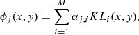
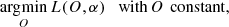
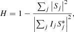
Figure 4 shows four representative cases obtained once the neural network is properly trained. The first column displays the deconvolved images, both the baseline result (labeled ‘MFBD’) and the resulting deconvolved image using the PSFs estimated by the neural network (‘labeled Neural’). We show results for the WB and only one of the two NB channels. The two NB channels are indeed very similar and their difference is proportional to the polarization, which is expected to be very small for many of the observed regions. The first and third columns display four of the seven available raw frames. It is clear that the multiframe blind deconvolution produces much better image quality with only seven frames, but our architecture can deal seamlessly with an arbitrary number of raw frames. The estimated PSFs are displayed in the second and fourth columns, which are shared by the WB and NB channels.
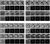 |
Fig. 4. Four examples of extended object deconvolution, each one showing results for the WB and one of the NB channels. Upper row: displays the baseline deconvolution together with four raw frames. Second and fourth rows: display the estimated PSFs by the neural network and the baseline, respectively. As NB and WB channels are simultaneous, the PSFs are shared for the two objects. |
5. Conclusions and outlook
We present a general scheme to train a neural multiframe blind deconvolution architecture without supervision. The method makes use of observed images only, together with information about the telescope entrance pupil, the angular pixel size in the camera, and the wavelength of the observations. We have shown, with examples obtained from the NOT with point-like objects and the SST with extended objects, that the neural deconvolution generalizes correctly to unseen images. The method also provides as output the instantaneous wavefronts produced by the atmospheric turbulence, irrespectively of the number of frames used. The method is extremely fast if compared with standard iterative blind deconvolution methods. The code for training or evaluation, with the parameters of the networks, is freely available2.
Given the fundamental ambiguities of inferring wavefronts from PSFs (Paxman et al. 2019), we do not consider that our method is especially competitive with more classical approaches based on, for instance, Shack-Hartmann sensors. However, our estimation of the instantaneous PSF is adequate for the deconvolution of images or spectra (van Noort 2017).
Our aim in this paper is to present the formalism for the unsupervised training. However, we point out that there are several possible ways of improving this work. The first one is to train an architecture that can blindly deconvolve images from a variety of telescopes and/or wavelengths. However, observations made using these telescopes and/or wavelengths are needed for the training. The formalism remains the same, except for the construction of the OTF from the generalized pupil. In this case, one needs to take into account the specific aperture of the telescope and the influence of the wavelength on the diffraction limit of the telescope. Apart from that, we anticipate that conditioning the entrance of the RNNs feature vector with the telescope properties and the wavelength should be sufficient. This can be easily done by concatenating this information on the input vector.
The second potential improvement is to add more training examples that have a larger variety of objects, especially extending it to other wavelengths of interest. However, we note that the convolutional part of the architecture that we have trained is in charge of obtaining relevant latent features from the image, from which a good estimation of the wavefront coefficients can be produced. As such, this CNN needs to learn how to be agnostic to the specific object, which can be difficult if the variability of objects is increased. This can easily be solved if more information is provided to the neural network. An obvious solution is to use a phase-diversity channel. The combination of the two images contains (theoretically) enough information to restrict the wavefront. Very preliminary experiments show that this addition strongly constrains the problem and produces wavefront coefficients of much better quality, which might then be competitive with those obtained with classical wavefront sensing methods.
Another restriction of our approach is that the input images are currently limited to be of a fixed size such that W is a multiple of 8. This is a consequence of the presence of the fully connected GRU and FC networks. This can be potentially solved by transforming our architecture into a fully convolutional one. Some convolutional counterparts of RNNs can be used, such as the ConvLSTM (Shi et al. 2015). Also, the FC network can then be transformed into a fully convolutional network. All networks can be trained with images of a certain size, and once trained can be applied to images of any other size. For instance, if the input images are of 128 × 128 pixels in size, the input to the ConvLSTM will be 16 × 16, meaning that at the output we would predict the wavefront in 16 × 16 patches of 8 × 8 pixels. For computing the loss function one would need a way to deal with these spatially variant PSFs. One option would be to compute the loss function locally in each patch and add them together.
Finally, although the GRU behaves correctly in our case, its serial character makes it slightly slow when training, meaning that it cannot be run in parallel. Recurrent neural networks have been improved in recent years by the use of more robust approaches. We plan to study the application of ‘transformers’ (Vaswani et al. 2017), which can better exploit the time information of the observations.
Acknowledgments
We thank Michiel van Noort for several invaluable discussions during the development of this work and for insisting on the interest of a machine learning approach to infer wavefronts in addition to the deconvolved image. We thank Álex Oscoz, Roberto López and Jorge Andrés Prieto for providing the FastCam@NOT datasets and Jaime de la Cruz Rodríguez for providing the CRISP@SST datasets. This study was also discussed in the workshop Studying magnetic-field-regulated heating in the solar chromosphere (team 399) at the International Space Science Institute (ISSI) in Switzerland. This paper is based on observations made with the Nordic Optical Telescope operated by the Nordic Optical Telescope Scientific Association in the Spanish Observatorio del Roque de los Muchachos of the Instituto de Astrofísica de Canarias. We are very grateful to the ING staff and the IAC Support Astronomers Group for their efforts. We acknowledge financial support from the Spanish Ministerio de Ciencia, Innovación y Universidades through project PGC2018-102108-B-I00 and FEDER funds. This research has made use of NASA’s Astrophysics Data System Bibliographic Services. We acknowledge the community effort devoted to the development of the following open-source packages that were used in this work: numpy (numpy.org, Harris et al. 2020), matplotlib (matplotlib.org, Hunter 2007), PyTorch (pytorch.org, Paszke et al. 2019) and h5py (h5py.org).
References
- Abramowitz, M., & Stegun, I. A. 1972, Handbook of Mathematical Functions (New York: Dover) [Google Scholar]
- Asensio Ramos, A., de la Cruz Rodríguez, J., & Pastor Yabar, A. 2018, A&A, 620, A73 [NASA ADS] [CrossRef] [EDP Sciences] [Google Scholar]
- Babacan, S. D., Molina, R., Do, M. N., & Katsaggelos, A. K. 2012, in Computer Vision - ECCV 2012, eds. A. Fitzgibbon, S. Lazebnik, P. Perona, Y. Sato, & C. Schmid (Berlin, Heidelberg: Springer), 341 [CrossRef] [Google Scholar]
- Blanc, A., Mugnier, L. M., & Idier, J. 2003, J. Opt. Soc. Am. A, 20, 1035 [NASA ADS] [CrossRef] [Google Scholar]
- Blanco, L., & Mugnier, L. M. 2011, Opt. Express, 19, 23227 [NASA ADS] [CrossRef] [Google Scholar]
- Bucci, O. M., Capozzoli, A., & D’Elia, G. 1999, J. Opt. Soc. Am. A, 16, 1759 [CrossRef] [Google Scholar]
- Cho, K., Merrienboer, B. V., Gülçehre, Çaglar, et al. 2014, EMNLP [Google Scholar]
- Clevert, D. A., Unterthiner, T., & Hochreiter, S. 2015, Under Review of ICLR2016 (1997) [Google Scholar]
- de la Cruz Rodríguez, J., Löfdahl, M. G., Sütterlin, P., Hillberg, T., & Rouppe van der Voort, L. 2015, A&A, 573, A40 [NASA ADS] [CrossRef] [EDP Sciences] [Google Scholar]
- Denis, L., Thiébaut, É., Soulez, F., Becker, J.-M., & Mourya, R. 2015, Int. J. Comput. Vision, 115, 253 [CrossRef] [Google Scholar]
- Farrens, S., Ngolè Mboula, F. M., & Starck, J. L. 2017, A&A, 601, A66 [NASA ADS] [CrossRef] [EDP Sciences] [Google Scholar]
- Fétick, R. J. L., Mugnier, L. M., Fusco, T., & Neichel, B. 2020, MNRAS, 496, 4209 [CrossRef] [Google Scholar]
- Gonsalves, R. A., & Chidlaw, R. 1979, in SPIE Conf. Ser., ed. A. G. Tescher, 207, 32 [Google Scholar]
- Harris, C. R., Millman, K. J., van der Walt, S. J., et al. 2020, Nature, 585, 357 [CrossRef] [PubMed] [Google Scholar]
- Herbel, J., Kacprzak, T., Amara, A., Refregier, A., & Lucchi, A. 2018, J. Cosmol. Astropart. Phys., 2018, 054 [NASA ADS] [CrossRef] [Google Scholar]
- Hirsch, M., Sra, S., Schölkopf, B., & Harmeling, S. 2010, Proceedings of the 23rd IEEE Conference on Computer Vision and Pattern Recognition, Max-Planck-Gesellschaft (Piscataway, NJ, USA: IEEE), 607 [Google Scholar]
- Hirsch, M., Harmeling, S., Sra, S., & Schölkopf, B. 2011, A&A, 531, A9 [NASA ADS] [CrossRef] [EDP Sciences] [Google Scholar]
- Hochreiter, S., & Schmidhuber, J. 1997, Neural Comput., 9, 1735 [CrossRef] [PubMed] [Google Scholar]
- Hunter, J. D. 2007, Comput. Sci. Eng., 9, 90 [NASA ADS] [CrossRef] [Google Scholar]
- Ioffe, S., & Szegedy, C. 2015, Proceedings of the 32Nd International Conference on International Conference on Machine Learning - Volume 37, ICML’15, 448 [Google Scholar]
- Kingma, D. P., & Ba, J. 2014, ArXiv e-prints [arXiv:1412.6980] [Google Scholar]
- Labeyrie, A. 1970, A&A, 6, 85 [Google Scholar]
- Löfdahl, M. G., & Scharmer, G. B. 1994, A&As, 107, 243 [Google Scholar]
- Löfdahl, M. G., Berger, T. E., Shine, R. S., & Title, A. M. 1998, ApJ, 495, 965 [NASA ADS] [CrossRef] [Google Scholar]
- Löfdahl, M. G., Bones, P. J., Fiddy, M. A., & Millane, R. P. 2002, in Image Reconstruction from Incomplete Data, 4792, 146 [NASA ADS] [CrossRef] [Google Scholar]
- Markham, J., & Conchello, J.-A. 1999, J. Opt. Soc. Am. A, 16, 2377 [CrossRef] [Google Scholar]
- Möckl, L., Petrov, P. N., & Moerner, W. E. 2019, Appl. Phys. Lett., 115, 251106 [CrossRef] [Google Scholar]
- Molina, R., Nunez, J., Cortijo, F. J., & Mateos, J. 2001, IEEE Signal Process. Mag., 18, 11 [NASA ADS] [CrossRef] [Google Scholar]
- Mugnier, L. M., Fusco, T., & Conan, J.-M. 2004, J. Opt. Soc. Am. A, 21, 1841 [NASA ADS] [CrossRef] [Google Scholar]
- Nagy, J. G., & O’Leary, D. P. 1998, SIAM J. Sci. Comput., 19, 1063 [CrossRef] [Google Scholar]
- Noll, R. J. 1976, J. Opt. Soc. Am., 66, 207 [NASA ADS] [CrossRef] [Google Scholar]
- Oscoz, A., Rebolo, R., López, R., et al. 2008, Proc. SPIE, 7014, 701447 [CrossRef] [Google Scholar]
- Paszke, A., Gross, S., Massa, F., et al. 2019, in Advances in Neural Information Processing Systems, eds. H. Wallach, H. Larochelle, A. Beygelzimer, et al. (Curran Associates, Inc.), 32, 8024 [Google Scholar]
- Paxman, R. G., Schulz, T. J., & Fienup, J. R. 1992, J. Opt. Soc. Am. A, 9, 1072 [NASA ADS] [CrossRef] [Google Scholar]
- Paxman, R. G., Seldin, J. H., Loefdahl, M. G., Scharmer, G. B., & Keller, C. U. 1996, ApJ, 466, 1087 [NASA ADS] [CrossRef] [Google Scholar]
- Paxman, R. G., Carrara, D. A., Miller, J. J., et al. 2019, in Unconventional and Indirect Imaging, Image Reconstruction, and Wavefront Sensing 2019, eds. J. J. Dolne, M. F. Spencer, & M. E. Testorf, Int. Soc. Opt. Photonics (SPIE), 11135, 106 [Google Scholar]
- Rigaut, F. 2015, PASP, 127, 1197 [CrossRef] [Google Scholar]
- Roddier, N. 1990, Opt. Eng., 29, 1174 [NASA ADS] [CrossRef] [Google Scholar]
- Shi, X., Chen, Z., Wang, H., et al. 2015, Proceedings of the 28th International Conference on Neural Information Processing Systems - Volume 1, NIPS’15 (Cambridge, MA, USA: MIT Press) [Google Scholar]
- Thelen, B. J., Paxman, R. G., Carrara, D. A., & Seldin, J. H. 1999, J. Opt. Soc. Am. A, 16, 1016 [NASA ADS] [CrossRef] [Google Scholar]
- Tipping, M. E., & Bishop, C. M. 2002, in Proceedings of the 15th International Conference on Neural Information Processing Systems, NIPS’02 (Cambridge, MA, USA: MIT Press), 1303 [Google Scholar]
- van Noort, M. 2017, A&A, 608, A76 [NASA ADS] [CrossRef] [EDP Sciences] [Google Scholar]
- van Noort, M., Rouppe van der Voort, L., & Löfdahl, M. G. 2005, Sol. Phys., 228, 191 [Google Scholar]
- Vaswani, A., Shazeer, N., Parmar, N., et al. 2017, in Advances in Neural Information Processing Systems, eds. I. Guyon, U. V. Luxburg, S. Bengio, et al. (Curran Associates, Inc.), 30, 5998 [Google Scholar]
- von der Lühe, O. 1993, A&A, 268, 374 [NASA ADS] [Google Scholar]
- Weigelt, G. 1977, Opt. Commun., 21, 55 [NASA ADS] [CrossRef] [Google Scholar]
- Wieschollek, P., Hirsch, M., Schölkopf, B., & Lensch, H. 2017, IEEE International Conference on Computer Vision (ICCV 2017), 231 [CrossRef] [Google Scholar]
All Tables
All Figures
|
Fig. 1. Block diagrams showing the architecture of the network and how it is trained unsupervisedly. The details of each layer are specified in Table 1 and in Sect. 2.5. |
| In the text | |
|
Fig. 2. Original frames of the burst (first row), estimated PSF with the neural approach (second row) and the baseline (fourth row), together with the reconstructed individual images (third and fifth rows). Several sources with different seeing conditions and characteristics are displayed. |
| In the text | |
|
Fig. 3. Time evolution of the first 36 coefficients of the phase in the KL basis in radians for the σ-Ori observation. The parameters found by the classical MFBD solution are shown in blue, while those inferred by the neural network are shown in orange. |
| In the text | |
|
Fig. 4. Four examples of extended object deconvolution, each one showing results for the WB and one of the NB channels. Upper row: displays the baseline deconvolution together with four raw frames. Second and fourth rows: display the estimated PSFs by the neural network and the baseline, respectively. As NB and WB channels are simultaneous, the PSFs are shared for the two objects. |
| In the text | |
Current usage metrics show cumulative count of Article Views (full-text article views including HTML views, PDF and ePub downloads, according to the available data) and Abstracts Views on Vision4Press platform.
Data correspond to usage on the plateform after 2015. The current usage metrics is available 48-96 hours after online publication and is updated daily on week days.
Initial download of the metrics may take a while.