| Issue |
A&A
Volume 646, February 2021
|
|
|---|---|---|
| Article Number | A115 | |
| Number of page(s) | 14 | |
| Section | Extragalactic astronomy | |
| DOI | https://doi.org/10.1051/0004-6361/202038343 | |
| Published online | 17 February 2021 | |
Electron-beam interaction with emission-line clouds in blazars
1
Universität Würzburg, 97074 Würzburg, Germany
e-mail: cwendel@astro.uni-wuerzburg.de
2
Inst. de Astrofísica de Canarias, 38200 La Laguna, Spain
e-mail: jbecerra@iac.es
3
Universidad de La Laguna, Dpto. Astrofísica, 38206 La Laguna, Tenerife, Spain
4
Max-Planck-Institut für Physik, 80805 München, Germany
e-mail: dpaneque@mppmu.mpg.de
Received:
4
May
2020
Accepted:
7
December
2020
Context. An electron-positron beam escaping from the magnetospheric vacuum gap of an accreting black hole interacts with recombination-line photons from surrounding gas clouds. Inverse-Compton scattering and subsequent pair production initiate unsaturated electromagnetic cascades exhibiting a characteristic spectral energy distribution.
Aims. By modelling the interactions of beam electrons (positrons) with hydrogen and helium recombination-line photons, we seek to describe the spectral signature of beam-driven cascades in the broad emission-line region of blazar jets.
Methods. Employing coupled kinetic equations for electrons (positrons) and photons including an escape term, we numerically obtained their steady-state distributions and the escaping photon spectrum.
Results. We find that cascade emission resulting from beam interactions can produce a narrow spectral feature at TeV energies. Indications of such an intermittent feature, which defies an explanation in the standard shock-in-jet scenario, have been found at ≈ 4σ confidence level at an energy of ≈ 3 TeV in the spectrum of the blazar Mrk 501.
Conclusions. The energetic requirements for explaining the intermittent 3 TeV bump with the beam-interaction model are plausible: Gap discharges that lead to multi-TeV beam electrons (positrons) carrying ≈ 0.1% of the Blandford-Znajek luminosity, which interact with recombination-line photons from gas clouds that reprocess ≈ 1% of the similar accretion luminosity are required.
Key words: galaxies: active / BL Lacertae objects: individual: Markarian 501 / quasars: emission lines / acceleration of particles / scattering / radiation mechanisms: non-thermal
© ESO 2021
1. Introduction
The launching of astrophysical jets from accreting black holes (BHs) involves fundamental gravitomagnetic processes. The frame-dragging effect on the plasma of the inner accretion flow and its advected magnetic field creates a rotating magnetosphere that can lead to a vacuum voltage drop of 1020 eV for a typical spinning supermassive BH in the centres of galaxies (Levinson & Rieger 2011). It is commonly thought that thermal pair production (PP) in photon-photon collisions provides charge carriers in sufficient numbers to supply the Goldreich-Julian density, which allows electric currents to remove the space charges resulting from the electric potential and to reshape the magnetosphere into a force-free configuration. Any imbalance in the supply of charged particles, however, results in the immediate creation of vacuum (electrostatic) gaps. In vacuum gaps the actual charge density, provided by photon-photon PP (see, however, Petropoulou et al. 2019, for an assessment of the importance of triplet PP in limiting the gap growth), is different from the Goldreich-Julian charge density. Because of this deviation, the force-free condition is not satisfied and the electric field component parallel to the magnetic field lines is non-vanishing and able to accelerate intruding charge carriers to relativistic velocities, extracting energy from the central rotating BH (Blandford & Znajek 1977; Beskin et al. 1992; Hirotani & Okamoto 1998; Levinson 2000).
The interaction of a particle beam with a low-energy radiation field results in electromagnetic cascades. Inverse-Compton (IC) scattering of the primary electrons off low-energy photons produces gamma rays that then undergo PP by interacting with the same photon field leading to a secondary generation of electrons. This sequence repeats until the gamma rays can escape freely (Lovelace et al. 1979; Akharonian et al. 1985; Svensson 1987; Zdziarski 1988; Aharonian & Plyasheshnikov 2003).
Cascades have been studied in a variety of astrophysical environments. In outer magnetospheric vacuum gaps of pulsars, curvature radiation is thought to initiate the pair cascade, limiting the gap growth by supplying charged particles (cf. Cheng et al. 1986; Hirotani 2005; Tang et al. 2008). The gamma rays produced by the cascade and leaving the pulsar magnetosphere in a confined beam are made responsible for the observed high-energy (HE) and very high energy (VHE) pulsed emission. In the galactic centre, vacuum gaps are hypothesised to drive cascades that are responsible for PeV cosmic rays and for the VHE gamma-ray point source coincident with Sagittarius A* (cf. e.g., Levinson & Rieger 2011; Katsoulakos et al. 2020).
In active galactic nuclei (AGN) with high accretion rates such as Seyfert galaxies, IC pair cascades in the coronal plasma of the accretion disk are thought to shape their X-ray spectrum up to MeV energies (Svensson 1987; Zdziarski 1988). In AGN with jets such as blazars, unsaturated IC pair cascades can develop from which gamma rays at energies well above MeV can escape. The cascades can be initiated by relativistic particles accelerated in vacuum gaps in the BH magnetosphere when the accretion rate is too low to supply the Goldreich-Julian density but their magnetic field is strong enough to launch a jet (Neronov & Aharonian 2007; Neronov et al. 2009; Levinson & Rieger 2011; Hirotani et al. 2017; Katsoulakos & Rieger 2020; Hirotani 2018, for a review). The gaps are thought to be located at the poles of the spinning BH magnetosphere near to the null surface where the Goldreich-Julian charge density is equal to zero (Beskin et al. 1992; Hirotani & Okamoto 1998; Ptitsyna & Neronov 2016; Hirotani et al. 2016; Levinson & Segev 2017; Ford et al. 2018; Chen & Yuan 2020; Kisaka et al. 2020). It was also found that gaps form around the divide of the magnetohydrodynamic (MHD) flow, called the stagnation surface (Vincent & Lebohec 2010; Broderick & Tchekhovskoy 2015; Hirotani & Pu 2016; Aharonian et al. 2017), or near to the inner light surface of the magnetosphere (Crinquand et al. 2020). Time-dependent one-dimensional, general relativistic MHD simulations by Levinson & Segev (2017), Levinson & Cerutti (2018), Chen et al. (2018), and Chen & Yuan (2020) and two-dimensional simulations by Crinquand et al. (2020, for computational reasons, the latter authors had to restrict themselves to unrealistic parameters, however) have recently found inherently non-stationary gap solutions. Levinson & Cerutti (2018) and Kisaka et al. (2020) indicate that the gap activity relaxes to low-amplitude quasi-steady oscillations after an initial spark event, while Chen et al. (2018) and Chen & Yuan (2020) find cyclically enduring gap activity.
Gap-accelerated particles then interact with ambient photon fields, that is, photons from the accretion flow or from the broad line region (BLR), initiating the onset of a cascade (cf. Blandford & Levinson 1995; Broderick & Tchekhovskoy 2015), which gives rise to an additional component of IC up-scattered photons that are emitted along a beam in the same direction as the original electrons were moving. When these cascaded photons can escape from the AGN gamma sphere without being absorbed by PP, and when the line of sight coincides with the beam, the emission could cause an observable imprint on the spectral energy distribution (SED) of the AGN. Intermittency of the particle flux injected from the gap or of the target photon field results in time variability of the emerging radiation and in transient features of the total SED. This could serve as an explanation of the observed minute- and hour-scale variability of HE and VHE emission in blazars (cf. Aharonian et al. 2007; Albert et al. 2007; Foschini et al. 2013; Pittori et al. 2018; Liao 2018). Similar short-term variability has been found in AGN with jets at inclination angles larger than a few degrees, which supports a similar interpretation (cf. Aleksić et al. 2014; MAGIC Collaboration 2018). Alternative scenarios to explain the short-time variability are the interaction of the jet with the radiation field from a stellar envelope, for instance, or a relativistically propagating emission zone in a relativistically moving jet (cf. Aharonian et al. 2017; Rieger 2019).
In this paper, we examine IC pair cascades in blazars emphasising the interaction of beam electrons from (short-lived) vacuum gaps with recombination-line photons. Blazars are subdivided into two subclasses, flat-spectrum radio quasars (FSRQs) and BL Lacertae (BL Lac) objects (for a recent review, see e.g., Foschini 2017). These two types were originally distinguished by the presence of broad optical emission lines in the case of FSRQs, with equivalent width |Wλ| > 0.5 nm, and the absence of broad optical emission lines for BL Lac objects (Urry & Padovani 1995). However, even in BL Lac objects, in which by definition |Wλ| < 0.5 nm, optical and ultraviolet recombination lines from the BLR are often present (cf. Stocke et al. 2011; Becerra González et al. 2020, for Markarian 501 and S4 0954+65, respectively), and might imprint a diagnostically important signature on the gamma-ray spectra emerging from the innermost regions.
This paper is organised as follows: in Sect. 2 we describe the physical model for the beam-photon interaction scenario and its underlying assumptions, including the set of coupled kinetic equations that were employed to numerically evaluate the model. We outline the numerical procedure for solving them to obtain the steady-state particle and photon distributions in Sect. 3. In Sect. 4 we apply this numerical scheme to fit the observational SED of the BL Lac object Markarian 501 (Mrk 501), which exhibited a peculiar spectral feature at ≈ 3 TeV during a strong flaring activity in 2014 July (MAGIC Collaboration 2020), and discuss the implications of the proposed scenario for the jet formation in Mrk 501. Finally, Sect. 5 summarises our findings.
In the following me, c, e, σTh, kB, and h denote the electron rest mass, the velocity of light, the elementary charge, the Thomson cross section, the Boltzmann constant, and Planck’s constant, respectively. SI units are employed unless noted otherwise.
2. Unsaturated inverse-Compton pair cascade model
The electron beam from an active spark gap region close to the accreting BH can initiate IC pair cascades (Broderick & Tchekhovskoy 2015; Ptitsyna & Neronov 2016; Ford et al. 2018; Levinson & Cerutti 2018; Chen & Yuan 2020). When the beam electrons propagate further along the jet axis, they can encounter the intense photon field of an emission-line cloud as depicted in Fig. 1, and initiate IC pair cascades. Because the threshold energy for PP in photon-photon collisions with the optical and ultraviolet photons characteristic for recombination-line spectra is high, the cascade spectra do not saturate at the electron rest mass energy delivering X-ray spectra, but instead produce spectra peaking at VHE gamma rays. Such cascades are also linear because the reservoir of low-energy target photons is not modified by the cascade in a major way. For their SEDs, it is essential to consider an escape term accounting for the energy-dependent gamma sphere resulting from the pair creation optical depth, which decreases towards the edge of the emission region.
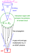 |
Fig. 1. Sketch of the geometry (not to scale) assumed for the model. Seed electrons are accelerated in the gap and multiplied in and behind the gap through ADAF photons. For simplicity of drawing, photons are not shown in the in-gap and post-gap multiplication. After propagating away from the gap, the electron beam meets an emission-line photon field, driving a cascade, whose steady-state gamma-ray photon density is nγ and whose escaping flux is Fcasc. To convert nγ into Fcasc, cf. Eq. (3). |
2.1. Unsaturated inverse-Compton pair cascade with escape
For the model of the emission region, we treated electrons and positrons identically and assumed three reservoirs of particle species to be present: firstly, we have relativistic electrons with spectral number density N(γ), where γ denotes the Lorentz factor of the electron. Secondly, we have highly energetic photons with spectral number density nγ(xγ), where xγ denotes the photon energy in units of the electron rest mass energy mec2. In what follows, the term “highly energetic photon” does not only denote photons with energies in the established HE range from 100 MeV to 100 GeV, but more generally photons with energies well above mec2, in contrast to low-energy photons with energies well below mec2. Thirdly, we have external low-energy photons with spectral number density n0(x) with x1 ≤ x ≤ x0 ≪ 1.
We assumed that all number densities are time-independent, isotropic, and homogeneous throughout the interaction region, and that interactions take place only inside of it. The interactions were assumed to be dominated by IC scattering and photon-photon PP. The cascade is then driven by PP from collisions in which the low-energy target photons turn the highly energetic photons into electron-positron pairs that then IC scatter off the same low-energy target photons to become the next generation of highly energetic photons, and so on (cf. Fig. 2). We considered four additional mechanisms acting as sinks or sources for the highly energetic photons or the electrons: first, there is the injection of highly energetic photons with spectral rate ṅγ,i(xγ) and xγ ≫ 1. Additionally, we demanded that the threshold condition for PP in collisions with the isotropic target radiation field with xγ x > 1 was fulfilled. Second, there is the injection of electrons with spectral rate Ṅi(γ). Henceforth, ṅγ,i and Ṅi are called spectral injection rate, and are defined as the number of particles, injected per unit space volume interval, per unit time interval, and per unit energy interval. We required that Ṅi is non-vanishing only for γ ≫ 1, hence the electrons have to be highly relativistic. Furthermore, we required that γ x > 1 was satisfied for the injected electrons. This is equivalent with primary IC scattering events being in the Klein-Nishina (KN) regime. According to Zdziarski (1988), this type of cascade is denoted IC-Klein-Nishina pair cascade. Third, there is escape of highly energetic photons from the interaction region with timescale Tph esc(xγ). Fourth, there is electron escape with timescale Te esc(γ). This is the main difference of our treatment to that by Zdziarski (1988) and Wendel et al. (2017), who considered saturated cascades; it makes our scenario more realistic. A finite escape timescale is equivalent to a bounded interaction region and is thus closer to reality than an infinite escape timescale, which is equivalent to an infinitely large interaction volume. The cascades considered here are therefore not necessarily saturated.
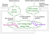 |
Fig. 2. Sketch of the considered linear IC pair cascade with escape terms. |
We assumed that the reservoir of target photons was not modified by the cascade. In other words, n0(x) is kept constant. This assumption is equivalent to assuming that a cascade is linear (Zdziarski 1988). Linearity of a cascade means that the low-energy photons alone serve as targets. Self-interactions of the highly energetic photons and of the electrons are neglected. Zdziarski (1988) showed by comparing cross sections that when the energy density of low-energy photons is at least similar to that of the highly energetic photons, the condition for a cascade to be linear is met whose interactions occur in the KN regime. Repetition of IC scattering events successively decreases the electron energy, until IC scattering events take place in the Thomson regime (γ x < 1). Here, cascades are always non-linear because xγ x < 1 implies that PP is not possible and thus PP is only possible through highly energetic photon self-interactions.
2.2. Description through kinetic equations
To determine the change rates of the spectral number densities of photons and electrons, we used the spectral interaction rates of IC scattering and of PP given by Zdziarski (1988).
For IC events with incident electrons of energy γ ≫ 1 scattering off photons with energy x ≪ 1 and spectral number density n0(x), which result in down-scattered electrons with energy γ′ and highly energetic photons with energy xγ, the spectral IC scattering interaction rate is denoted by C(γ, γ′) and determined with Eq. (A.1) by Zdziarski (1988), cf. Appendix A. For such events, the threshold γIC, th(xγ, x) as defined in Appendix A is the minimum required value of γ. The maximum possible γ is γIC, max(γ′,x), as outlined in Appendix A. Furthermore, we define  as the minimum possible γ′ and xγ, max(γ, x) as the maximum energy of the up-scattered photon.
Because of the interaction of highly energetic photons of energy xγ with low-energy photons of energy x and spectral number density n0(x), resulting in the PP of electrons of energy γ, the spectral PP interaction rate is called P(xγ, γ) and is computed with Eq. (B.1) of Zdziarski (1988), cf. Appendix A. The PP threshold, that is, the minimum required xγ, is defined as xγ, PP, th(γ, x) in Appendix A. The values of γ that can be reached are limited by γPP, min(xγ, x) and γPP, max(xγ, x), as described in Appendix A.
The kinetic equation of the electrons and of the photons ensues after all the relevant sinks and sources are specified. The change rate of the spectral number density of the electrons (electron energy distribution) is affected by the electron spectral injection rate Ṅi, the spectral loss rate (as the sum of the escape rate with timescale Te esc and of the IC down-scattering rate to lower energies), and by the production rate (as the sum of the IC down-scattering rate from higher energies and of the PP rate). Similarly, the change rate of the spectral number density of the photons is determined from the photon spectral injection rate ṅγ,i, the loss rate (which is the sum of the escape rate with timescale Tph esc and of the pair absorption rate), and the production rate ṅγ,IC.
Assuming steady state, we obtain, as shown in Appendix A,
where we have defined two contributions to the photon spectral number density. nγ, i describes the contribution that arises from the interplay of injection and escape and absorption losses, while nγ, IC describes the contribution that is achieved from the interplay of production through IC up-scattering and both losses. Exchanging γ and γ′ in Eq. (1) and plugging this into Eq. (A.8), we can eliminate nγ,
3. Numerical solution procedure
In this section, we outline explicit solutions for N(γ) and nγ(xγ).
The main task is to find solutions for N. This is done by solving Eq. (2) iteratively. The right-hand side of Eq. (2) directly incorporates γ, Tph esc, Te esc, N, Ṅi, ṅγ,i, C, P, and the functions in the integration borders, which have been defined in the previous section. C and P are known as soon as n0 has been specified. Hence, Eq. (2) can briefly be written as N(γ) = ℱ′(n0, Ṅi, ṅγ,i, Tph esc, Te esc, N, γ). As described in Sect. 2.1, the first five arguments of ℱ′ are quantities that describe the physical setting. Hence, they should be understood as input functions and have to be prescribed to specify the physical problem. When this is done, we obtain the equation N(γ) = ℱ(N, γ), where ℱ was defined accordingly. Now, we chose a sequence (γk)k = 1, …, κ of κ discrete values γk along which the kinetic equation is to be solved, in other words, along which N(γ) is to be determined. We write N(γk) = Nk for convenience. As a starting point of the iteration, we guessed an initial course Ninit(γ) of the function N(γ) and determined the corresponding sequence of values (Nk)k = 1, …, κ; jinit. In Appendix B, we discuss how the converged sequence is determined numerically.
We performed the iteration using the python3 language. To numerically compute the integrals with an infinite integration range, we restricted the integration range we used to a finite range. This is possible when n0(x), ṅγ,i(xγ), and Ṅi(γ) are equal to zero everywhere above an upper cut-off, which we denote by x0, xγ, 0, and by γi, 0, respectively.
To summarise, the physical setting is specified as soon as the following functions are defined: The low-energy photon spectral number density n0, the highly energetic photon spectral injection rate ṅγ,i, the electron spectral injection rate Ṅi, the highly energetic photon escape time Tph esc, and the electron escape time Te esc. By iterating, our code then determined the steady state N. When N was known, we used Eq. (1) to determine nγ, and from this, we obtained the spectral flux density Fcasc. This approach differs from that of Wendel et al. (2017). Therein, although Tph esc = Te esc = ∞ (no escape) was used in the kinetic equation, it was assumed that the IC up-scattered photons leave the interaction region from its shell-like boundary. Accordingly, Wendel et al. (2017) directly converted the photon spectral production rate (last term in Eq. (A.7)) into the observed spectral flux density. This appears to be a very crude approach because first it neglects that the injected highly energetic photons can also leave the interaction region (which we take into account by nγ, i in Eq. (1)), and second it assumes that all IC up-scattered photons escape from the boundary of the interaction region and that no IC up-scattered photons escape from its interior. On the one hand, this second assumption contradicts the Tph esc = Te esc = ∞ assumption and on the other hand it neglects the energy-dependent behaviour of photon attenuation (which we took into account through the division of the photon spectral injection and production rate (numerator of Eq. (1)) by the spectral loss rate (denominator of Eq. (1))).
Based on nγ, we determined the spectral flux density Fcasc of highly energetic photons (i.e. the number of photons per unit energy, per unit area, and per unit time) through
We assumed that the photons leave the interaction region, whose approximate radial size is Rph esc(xγ), only through a conical beam of opening angle ϕ and solid angle Ω = 4π ⋅ sin2(ϕ/4), and that D is the distance to the observer. The size of the interaction region is linked with the escape time of the photons and electrons. A natural choice for this would be Rph esc(xγ) = Tph esc(xγ) c. The division by mec2 arises because Fcasc is measured in m−2 s−1 J−1, while nγ is in units of m−3.
4. Indication of gap activity in Markarian 501
The numerical procedure described above is used below to explain a peculiar feature in the VHE spectrum of the blazar Mrk 501 during a flaring activity on 2014 July 19.
The broadband emission from blazars, and in particular from the high-synchrotron-peaked BL Lac object Mrk 501, is characterised by a two-bump structure. This emission is usually described within the one-zone synchrotron-self-Compton (SSC) framework (see e.g., Maraschi et al. 1992; Dermer & Giebels 2016). In this model, a blob of relativistic electrons is assumed to move along the jet that points towards the observer. The blob is permeated by a randomly distributed magnetic field, producing synchrotron radiation from the electrons. This radiation is responsible for the low-energy SED bump in blazars. The origin of the HE bump is typically ascribed to the IC scattering of the relativistic electrons with the synchrotron photons. In addition to the SSC scenario, other theoretical models have been proposed to explain the HE and VHE emission in blazars, involving hadronic components and IC pair cascading. Minute-scale variability spectral components mean that the standard one-zone SSC scenario may be insufficient and suggest that an additional sporadic emission component is emitted from the innermost regions of the jet, see Ahnen et al. (2018).
Recently, the MAGIC Collaboration (2020) has presented a two-week flare from Mrk 501, mainly detected in X-rays with the Swift satellite and in VHE gamma rays observed with the major atmospheric gamma-ray imaging Cherenkov (MAGIC) telescopes. During this flaring state, the source displayed hard X-ray spectra as well as the highest X-ray count rate detected by the Swift X-ray Telescope during its 15 years of operation. In coincidence with the peak of the X-ray count rate, which took place on 2014 July 19 (MJD 56857.98), a narrow feature in the TeV spectrum from the MAGIC telescopes was detected with a significance of 3σ − 4σ. This feature, located around 3 TeV, is inconsistent with the standard functions to describe the VHE spectra from blazars (power law, log-parabola, and log-parabola with exponential cut-off) at more than 3σ confidence level. The VHE spectrum on 2014 July 19 is better explained assuming a narrow component (a narrow log-parabola or a Gaussian function) in addition to a broad log-parabola. Such a double function fit is preferred with respect to a single log-parabola at 3.2σ − 4.5σ, depending on the a priori assumptions (details can be found in MAGIC Collaboration 2020). This was the first time that a narrow feature (not consistent with the usual smooth spectral functions) was found with a significance higher than 3σ in the VHE spectrum of Mrk 501, and any TeV blazar in general. Indications for similar (but statistically insignificant) spectral features at ≈ 2 TeV can be found by inspection of flare spectra reported by the very energetic radiation imaging telescope array system (VERITAS; cf. Fig. 8 of Abdo et al. 2011) and the MAGIC collaboration (cf. Fig. 10 of Ahnen et al. 2017).
Under the assumption that the spectral feature described above is real, three different theoretical scenarios were proposed by the MAGIC Collaboration (2020) to reproduce the narrow spectral feature: (a) a pileup in the electron energy distribution produced by stochastic acceleration, (b) a two-zone SSC model, and (c) a narrow emission from an IC pair cascade scenario induced by electrons accelerated in a magnetospheric vacuum gap. Details for the model describing scenario (c) are provided in this work. In the following, we evaluate the model we fitted to the observational data to infer its implications and consequences.
4.1. Specification of the modelled setting
We assumed a vacuum gap near to the poles of the Mrk 501 BH magnetosphere. The potential drop in the gap accelerates seed electrons to ultra-relativistic energies. The seed electrons enter the gap both through PP of gamma rays from the hot advection-dominated accretion flow (ADAF), and possibly through direct leakage from it (Neronov et al. 2009). Seed electrons that have been accelerated in the gap, leave it in the direction of the electric field (i.e. in the direction of the magnetic field), and propagate along a beam that is well collimated to an opening angle ≈ ϕ. During the propagation away from the gap, the seed electrons still encounter the ADAF photon field, and a post-gap cascade (Broderick & Tchekhovskoy 2015; Chen & Yuan 2020) occurs and increases the number of electrons by repeated curvature-radiation and IC emission and PP events. This post-gap cascade ceases when curvature-radiation emission becomes negligible and when IC scattering and PP can no longer be sustained by ADAF photons. Several tens or hundreds of Schwarzschild radii away from the gap, the beam of electrons is assumed to enter a region in which background photons from ionised gas clouds are present. This induces a cascade in this interaction region. This model is depicted in Fig. 1. For this cascade, the model of Sect. 2 was applied. The electron beam from the gap serves as electron injection mechanism in our model. We describe the electron spectral injection rate with the following cut-off Gaussian:
Here, γmean denotes the mean Lorentz factor of the injected electrons, and ς parametrises the width of the distribution. For the cut-off values we chose γi, 1 = γmean − 3.0 ς and γi, 0 = γmean + 3.0 ς, satisfying the condition γ ⋅ x > 1 (cf. Sect. 2.1). The normalisation of the Gaussian, which describes the total number of electrons that are injected per unit time and per unit space volume, is called KG.
Furthermore, we assumed that the external low-energy photons of the cascade are represented by emission-line photons from photo-ionised gas clouds in the surroundings of the Mrk 501 BH magnetosphere. Although Mrk 501, as a BL Lac object, does not have a prominent BLR, its BLR has clearly been confirmed observationally, possibly due to outshining by the boosted jet emission, due to a weak accretion rate, or due to the lack of ambient gas (cf. Moles et al. 1987; Stocke et al. 2011). After they are triggered by minor galaxy mergers, interstellar gas clouds, consisting mainly of hydrogen and helium (Wilms et al. 2000), can migrate from the host galaxy into its centre and thus into the central part of Mrk 501. Radiation from the accretion flow or from OB-type stars in the dense galactic centre will inevitably ionise passing clouds. As an effect of recombination, emission-line photons will be abundant in the proximity of the clouds. The external low-energetic photon field can also stem from the envelope of a post-main-sequence star with low metallicity (cf. e.g., Bednarek & Protheroe 1997; Barkov et al. 2010). In any case, we assumed that the interaction region was both penetrated by the electron beam and pervaded by emission-line photons, and consequently, that an IC pair cascade developed there. It is natural to describe the spectral number density by a sum of Dirac delta distributions,
Here, x0, i = h/(λ0, i me c), and λ0, i are the dimensionless energy, and the wavelength of the ith line, respectively. Kline, i gives the relative flux density contribution of the ith line. Precisely, Kline, i gives the flux density of the emission line i with respect to the flux density of a hypothetical hydrogen Balmer-β line. Accordingly, Kline, i/x0, i describes the relative number density contribution of the ith line. The parameter Klines is a measure for the photon total number density. We restricted the sum to the three typically most important hydrogen lines plus the most important helium line. We compiled these lines and their respective Kline, i based on the ultraviolet spectroscopic blazar observations by Pian et al. (2005) and on the synthetic photo-ionisation spectra by Abolmasov & Poutanen (2017). We list them in Table 1.
Four emission lines used as external low-energy target photons.
From an energetic point of view, the emission-line radiation is just a reprocessed fraction of the more luminous ADAF radiation. Nevertheless, we did not include the ADAF radiation in the target photon field. This is justified by the following geometrical argument. The emission of line photons in the ionised cloud is approximately isotropic. The interaction angles of injected electrons and photons are therefore equally distributed; the interaction angle is on average 90°. This also justifies the usage of the interaction rates C and P. In contrast, for interactions of electrons with ADAF photons the collision angle would be at best 90°, and on average smaller than 90°. Thus, glancing collisions occur, and for such interactions, the interaction rates are lower than for right-angled collisions. This results in increased interaction rates for the line photons in comparison to ADAF photons, and thus we can neglect the latter. Moreover, except for the reprocessed photons from the ionised cloud, reprocessed ADAF photons might be scarce in the surroundings of the beam due to low ambient gas density in the BL Lac object, which means that they drop out as target photons as well. We have to mention furthermore, that ADAF spectra usually extend to higher energies and x ≪ 1, which was assumed in the derivation of C and P, is satisfied only very critically.
We did not have injection of highly energetic photons in this setting. Therefore we set the photon spectral injection rate

To choose the escape timescales, we determined
In other words, we approximated the interaction volume as a spherical region with radius R. Electrons and photons have equal, and energy independent, that is, constant, escape timescales. The function Rph esc(xγ) in Eq. (3) is therefore also set equal to the parameter R.
4.2. Modelling results
According to the procedure outlined in Sect. 3, we determined N(γ), nγ(xγ), and Fcasc(xγ) of the cascade that evolves through interaction of the electrons originally stemming from the gap with the emission-line photons, such that Fcasc(xγ) was fitted to the narrow SED feature (MAGIC telescopes’ data) and a background SSC emission is fitted to the multi-wavelength SED. We understand KG, Klines, γmean, ς, R, and ϕ as fitting parameters, while we used the luminosity distance D = 149.4 Mpc (corresponding to redshift z = 0.034, dimensionless density parameter Ωm = 0.3 of matter, dimensionless density parameter ΩΛ = 0.7 of dark energy, Hubble constant H0 = 70 km s−1 Mpc−1) and the line contributions Kline, i given in Table 1. Because the electron beam penetrates into the interaction region from one direction, the kinematics of IC scattering and PP ensure that the highly energetic photons leave the interaction region in this same direction, hence along a beam of opening angle ϕ.
Interim results of the numerical procedure are shown in Figs. 3–5 and are discussed now.
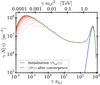 |
Fig. 3. γ N(γ), which is a proxy for the electron spectral energy density, versus the product of the Lorentz factor with the dimensionless energy of the highest energetic line, the helium II Lyman-α line. The iterated points Nk, j are drawn in red. |
The results of our iterative determination of N(γ) are shown in Fig. 3. The initial function of N was chosen to be
cf. Eq. (A.6). This choice is a compromise between a function that can be evaluated fast and is accurate. It is a good approximation for the final N in the highest energetic regime because the electron spectral production rate is negligible here. For decreasing γ, a higher number of iteration steps are necessary because the energy transfer in one IC scattering event decreases. We chose the convergence criterion as follows: One iteration was considered completed when the relative change |Nk, j − 1−Nk, j|/Nk, j between two successive values was smaller than 0.001 at the points  and smaller than 0.001 ⋅ (γkx0, 1/10)2 at the points
  . In other words, the demanded accuracy increases quadratically the deeper we iterate into the Thomson regime. There, about jfinal = 100 iteration steps were necessary to meet the convergence criterion, while only two or three steps were necessary in the KN regime, cf. Fig. 3. The shallow ridge of N at
  is caused by PP of highly energetic photons with hydrogen Lyman photons (mainly hydrogen Lyman-α photons), while the very shallow ridge at
  is caused by PP of highly energetic photons with the helium II Lyman-α photons. In other words, these ridges in N are the effect of peaks of the spectral PP rate (fourth summand in Eq. (A.6)). In the Thomson regime, with decreasing γ the course of N deviates more and more from the ∼ γ−2 dependence of the saturated cascade case considered by Zdziarski (1988) because particles escape in our scenario. The finite value of the escape time prevents the electrons from penetrating deep into the Thomson regime.
Figure 4 clearly shows that the photon spectral loss rate is dominated by pair absorption in the approximate range  corresponding to a photon energy between 19 GeV and 5.1 TeV, and by escape outside this energy range. The maximum of the photon spectral loss rate occurs at
  , corresponding to the maximum of the hydrogen Lyman-α absorption. The optical depths, which correspond to the respective spectral loss rate contributions, are shown in Fig. 4 on the right-hand side ordinate and were determined by multiplication of the respective spectral loss rate contribution with the escape time Tesc.
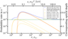 |
Fig. 4. Various contributions (cf. Eq. (A.7)) to the photon spectral loss rate on the left-hand side ordinate in dependence on the product of the dimensionless highly energetic photon energy with the dimensionless energy of the highest energetic line. On the right-hand side ordinate, we plot the optical depth that corresponds to the respective contribution to the spectral loss rate. |
We show the photon spectral production rate ṅγ,IC in Fig. 5. From N, it inherits the peak around  as well as the deviation from a power law in the Thomson regime due to escape (cf. Zdziarski 1988). In this figure we also show the spectral number density nγ of highly energetic photons. The contribution nγ, i vanishes because of the choice Eq. (6). The contribution nγ, IC is non-vanishing and ensues as a consequence of IC scattering, pair absorption, and escape. The pronounced trough above
  is due to absorption by PP with photons from the hydrogen Lyman-α line (cf. Fig. 4). Because of the smallness of Kline, 2 and Kline, 3, absorption features of the hydrogen Lyman-β line and series are almost invisible. The shallow dip of the spectral number density above
  is due to absorption on the helium II Lyman-α line. Thus, the slight bump at
  results from cascaded photons that are immediately below the threshold for PP and hence are not absorbed. The peaky feature around
  is more pronounced in nγ than in ṅγ,IC because the spectral loss rate (i.e. the denominator of nγ, IC) is higher below
  than at
  . If n0 were continuous and distributed along a wider range of x instead of consisting of a few strong lines, the peak around
  would be wider and extend to lower energies.
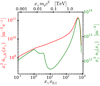 |
Fig. 5. Spectral production rate and number density of the cascade in Mrk 501. The product of the squared dimensionless photon energy with the spectral production rate of photons is plotted in red (which is determined by the last term of Eq. (A.7)). We show the product of the squared dimensionless photon energy with the spectral number density of photons in green (which is determined by Eq. (1)). Both quantities are plotted vs. the product of the highly energetic photon energy with the energy of the helium II Lyman-α line. |
The total energy density of highly energetic photons is obtained by integrating the spectral energy density xγ nγ(xγ)
The total energy density of the low-energy photons is  J m−3 and thus of similar magnitude. Our cascade is therefore indeed linear (cf. Sect. 2.1).
The cascaded spectral flux density Fcasc of highly energetic photons adds to the spectral flux density FSSC of photons that is produced farther downstream the jet in a common one-zone SSC scenario. Both these components contribute to the observed spectral flux density F. We fit both components, FSSC and Fcasc, to the multi-wavelength data of Mrk 501 of the night of MJD 56857.98 as presented by the MAGIC Collaboration (2020). As shown in Fig. 10 of MAGIC Collaboration (2020) and in Fig. 6 in the present paper, we can describe the narrow SED feature without the need of extreme SSC parameters. The parameters found by the fit are given for the cascaded emission component in Table 2 of the present paper and for the SSC emission component in Table 6 and Fig. 7 in MAGIC Collaboration (2020). The emission from a cascade initiated by electrons originating from a vacuum gap can thus explain the observed narrow peak-like feature.
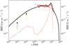 |
Fig. 6. High-energy bump of the SED of Mrk 501 from 2014 July 19 (MJD 56857.98). The dashed grey line depicts the IC bump of a one-zone SSC model (contribution FSSC). The dot-dashed red line depicts the emission of the cascade (contribution Fcasc, cf. green line in Fig. 5). The sum F of both contributions is depicted by the solid black line. The spectral data from the MAGIC telescopes are shown as red circles, while measurements and upper limits by the Fermi Large Area Telescope are drawn by black and yellow triangles. The details on the data analysis and the SSC modelling can be found in MAGIC Collaboration (2020). |
Fitting parameters that were used to describe the narrow SED feature by emission from an IC pair cascade.
4.3. Physical inferences
In this subsection we discuss the results of modelling Mrk 501. We assess the findings in a broader context.
4.3.1. Number and size of emission-line clouds
We compared the assumed hydrogen Lyman-α photon abundance with the hydrogen Lyman-α luminosity of LLy α, obs = 5.2 × 1033 W that was detected from Mrk 501 by Stocke et al. (2011). The total number density of all low-energy photons is given by  m−3. This number density describes the photon field of the ionised cloud assumed to be interacting with the electron beam from the gap. The total number density of hydrogen Lyman-α photons is determined by Klines ⋅ Kline, 4/x0, 4 ≈ 2.6 × 10¹⁸ m−3. We further assumed that there are Ncl clouds of approximate radial size Rcl in the BLR. The hydrogen Lyman-α luminosity LLy α, cl of all these clouds is responsible for the observed hydrogen Lyman-α luminosity. We can set

As BL Lac objects are considered to be evolved objects running short of cold gas supplies (Liodakis 2018; Foschini 2017), we can assume that Ncl is quite small. On the other hand, to obtain a Gaussian line profile for the emission lines resulting from the Doppler broadening, the number of clouds must not be too small. Then, solving Eq. (10) for the radial size yields an estimate of Rcl. Choosing Ncl = 10 yields Rcl ≈ 1.8 × 10¹¹ m, which roughly agrees with our value used for the radial size of the interaction region R (cf. Table 2). This size of the cloud corresponds to the size of a red giant, which is suggestive of cloud formation by photospheric abrasion through beam interaction. In terms of Schwarzschild radii rS for a central BH of mass M = 109 M⊙, it is Rcl = 0.061 rS. From the modelling we infer that in Mrk 501 only few major gas clouds are present in the BLR. The encounter of a major cloud with electrons from the gap-beam must therefore be a rare event. Presuming that the gas clouds revolve around the BH on unperturbed Keplerian orbits, an encounter of a cloud with the beam of electrons will at best repeat with the Keplerian orbital period of the cloud. These conclusions are in line with the fact that the peak-like SED feature has not been found elsewhere in Mrk 501 data.
4.3.2. Reprocessing of the accretion flow luminosity
The total line luminosity of these Ncl clouds of radius Rcl is determined as
For the above chosen Ncl = 10 and resulting Rcl = 1.8 × 10¹¹ m, it is Llines, tot ≈ 7.8 × 1033 W, a factor 5 lower than the upper limit of the Mrk 501 BLR luminosity found by Celotti et al. (1997). We recall that this finding was obtained from our modelling and from the observed hydrogen Lyman-α luminosity. In canonical BLR models, the BLR luminosity is assumed to be about 10% of the accretion flow luminosity (Ghisellini et al. 2017). As Mrk 501 is a gas-depleted object, its BLR reprocesses even less of the incident accretion flow radiation. Thus, the reprocessing fraction ξ = Llines, tot/LADAF, tot might be lower than 10%, say 1%. Here, LADAF, tot is the total luminosity of the ADAF. To compare the emission-line luminosity with the accretion flow luminosity, we applied the synthetic ADAF spectrum computed by Mahadevan (1997). There, the spectral luminosity of an ADAF as a function of frequency was parametrised by the viscosity parameter α, the pressure ratio β, the inner boundary Rin of the hot accretion flow, its outer boundary Rout, the central BH mass M, the electron temperature Te, and by the dimensionless mass accretion rate ṁ, which is defined as the ratio of the mass accretion rate to the Eddington accretion rate. We integrated numerically, and for the purpose of cross checking also analytically, along the photon energy ϵ over the spectral luminosity LADAF(ϵ) to obtain LADAF, tot. We integrated essentially over the superposition of the cyclosynchrotron emission, its Comptonised part, and of the bremsstrahlung contribution. We used the canonical choices α = 0.3, β = 0.5, Rin = 3 rS, and Rout = 1000 rS as well as M = 109 M⊙. Furthermore, we chose the energy ϵADAF, 0 = 300 kB Te as an upper integration border because the spectrum essentially vanishes above this energy. We let ṁ and Te be free parameters. The chosen requirement Llines,tot ≈ 0.01 · LADAF,tot(ṁ, Te) can be met with the exemplary ṁ, Te) pairs listed in row 1 of Table 3. This shows that the present scenario fits the general picture of accretion flows as illuminators of BLRs. Moreover, it gives evidence that Mrk 501 is indeed fed by a low-rate, hot ADAF. When the reprocessing fraction ξ is increased from 1% to the canonical 10%, the values of Te decrease by about 25% (cf. Table 3).
Four combinations of physical quantities connecting ADAF properties to the materialisation rate in the vacuum gap.
4.3.3. Constraints on the in-gap and post-gap multiplication
The parameter KG expresses the number density of electrons that intrude into the interaction region per time interval. In our model, these electrons enter the interaction region after their number was increased in the gap and during the post-gap cascade. The origin of the electron beam along which the multiplication takes place is the vacuum gap (cf. Fig. 1), where in turn the origin of the seed electrons is PP through self-interaction of ADAF radiation. In other words, photons that are emitted by the ADAF can collide in the BH magnetosphere and pair-produce seed electrons. We can determine the number density of ADAF photons capable of PP with the help of the ADAF model by Mahadevan (1997). The spectral number density of ADAF photons is given by nADAF(ϵ) = LADAF(ϵ)/(c ⋅ ϵ ⋅ AADAF), where  is a rough estimate of the surface area of the ADAF. We determined the total surface area as a sum of the outer cylindrical lateral area and the inner cylindrical lateral area, and twice the outer conical lateral was subtracted by the inner conical lateral area. Additionally, we assumed the height of the ADAF to be r at radius r. As mentioned above, the ADAF spectrum is non-vanishing up to the energy ϵADAF, 0. Because PP is a threshold process, the lowest possible ADAF photons capable of PP have the energy
  . Consequently, the total number density of ADAF photons capable of PP is obtained by
As a comparison, we determined the total number density of pair-producing MeV photons based on the approximation
from Levinson & Rieger (2011), which is motivated by findings for the bremsstrahlung luminosity of an ADAF by Narayan & Yi (1995). For the ADAF parameters we used above, the assumed ξ = 1%, and the constrained pairs of ṁ and Te, we give the correspondingly values of nPP, 1 and nPP, 2 in the second and third row of Table 3. Except for the last pair, we have an order-of-magnitude agreement. In contrast, for the canonical ξ = 10% and the corresponding lower Te, we obtain values for nPP, 1 that are about two orders of magnitude lower (cf. Table 3) than in the 1% reprocessing fraction case.
From the number density of pair-producing ADAF photons, we estimated the materialisation rate in the gap. With 0.2 σTh as an approximation for the PP cross section, the number density of pairs that are produced in the gap region per unit time is  . We show the values of KPP, gap for the ṁ, Te) pairs in the fourth row of Table 3. All four estimates in the ξ = 1% case are about six orders of magnitude smaller than our determined KG and all four estimates in the ξ = 10% case are about ten orders smaller. This does not necessarily cast doubt on our model.
These pair-produced seed electrons are accelerated in the gap and multiplied in the gap and during the propagation to the interaction with the emission-line photons. The multiplication is mediated by the emission of synchro-curvature radiation in the magnetospheric magnetic field, by the emission of IC up-scattered radiation in the ADAF photon field, and by the subsequent materialisation of this radiation through PP. In net effect, this multiplication increases the number of electrons by the number 𝒩 and also lowers the energy per electron by 𝒩. Because we neither included the magnetic field and the emission of synchro-curvature radiation nor the exact spatial distribution of the ADAF photon field into our model, a detailed analysis of the in-gap and post-gap multiplication is beyond the scope of this work. We can, however, estimate from comparison of KPP, gap with KG that it has to be 𝒩 ≈ 106 in the 1% reprocessing fraction case and 𝒩 ≈ 1010 in the 10% case. The finding 𝒩 ≈ 106 is three orders of magnitude larger than the multiplication found by Broderick & Tchekhovskoy (2015). These authors, however, determined the multiplication only in the post-gap cascade. Considering that up to 107 curvature photons can be emitted by one electron in the initial spark event of the gap (Levinson & Cerutti 2018), 𝒩 ≈ 106 after the post-gap cascade is plausible and does not inhibit gap stability. Furthermore, to assess the magnitude of 𝒩, we have to consider the magnetic field structure (especially the divergence of the magnetic field), which can dilute the number density of the electron bunch.
The maximum potential drop in the gap is connected with the maximum Lorentz factor of the electrons. Knowing from our modelling (cf. Eq. (4) and Table 2) that the maximum energy per electron after the multiplication is γi, 0 mec2 = (γmean + 3 ς) mec2 = 5.7 × 10¹² eV, we can estimate that the maximum energy that one original seed electron has attained in the gap voltage is ≈ 𝒩 ⋅ γi, 0 mec2. In the ξ = 1% case, this gives ≈ 5.7 × 10¹⁸ eV, which agrees with estimated (Levinson & Rieger 2011) and simulated (Hirotani & Pu 2016) values for the potential drop in a vacuum gap. In the ξ = 10% case, this gives ≈ 5.7 × 10²² eV, which seems hard to reach even for extreme magnetospheric gap conditions. Thus, the canonical choice ξ = 10% for the reprocessing fraction does not fit a consistent picture of Mrk 501. Levinson & Segev (2017), Levinson & Cerutti (2018), Chen & Yuan (2020), Crinquand et al. (2020), and Kisaka et al. (2020) have recently cast doubt on the prior attitude of vacuum gaps being steady-state phenomena. Instead, they might be of intermittent or cyclic character. In particular, Levinson & Cerutti (2018) found that charge-starved gaps, after ignition by injection of gamma rays or electrons abruptly discharge in a gamma-ray flaring event on a timescale rS/(2c), followed by relaxation towards a state of weak-amplitude oscillations of the electric field and plasma. In this case, rule-of-thumb estimates for the maximum potential drop would not be adequate for conclusions about the attained electron Lorentz factor. We therefore leave detailed inferences from our input parameters about conditions in the vacuum gap to future studies.
If the electron beam is emitted from an oscillating gap, we might expect that this also leads to cyclic behaviour of the cascade with the emission-line photons. However, Broderick & Tchekhovskoy (2015) found that if the gap width exceeds its height, then the gap consists of a number of causally independent tubes. The cyclic behaviour after the initial spark can therefore hardly be traced because the emitted electron beam is the transverse average of many independently fluctuating gap tubes.
4.3.4. Comparison of energy budgets
The total power that is injected into the interaction volume is determined to be  W, where R is the radial size of the interaction region. This power is due to the electrons that have inherited their energy from gap acceleration. Hence, Pi has to be smaller than the maximum power Pgap that can be extracted from the gap, which itself cannot exceed the corresponding Blandford-Znajek power PBZ. Moreover, we determine the power, that is radiated by the electrons in the SSC emitting zone to be PSSC = 4.4 × 1036 W.
The magnetic flux density at the BH horizon upon assuming an open gap was estimated by Aharonian et al. (2017) to be BBH = 0.19 ⋅ (βm/M9)4/7 T, where βm is the magnetisation of the ADAF. Assuming the maximum possible electric field strength, gap extension, BH spin, and charge density, Aharonian et al. (2017) obtained  W, where we have substituted for the variability timescale by the height h of the gap in units of Schwarzschild radii, and where θ is the polar angle, and κ is the multiplicity in the gap as defined by Aharonian et al. (2017). For the values θ = π/4, κ = 0.1 (weakly screened gap), h = 0.25 (thickness is half a gravitational radius), and βm = 0.5 (magnetic pressure is half the gas pressure), we find Pgap = 2.7 × 1035 W. For the same parameters and for the dimensionless BH spin parameter a* = 0.99, we find
  W (Hirotani et al. 2016), which is twice the accretion flow luminosity (cf. Sect. 4.3.2).
To conclude, we find Pi/PBZ ≈ 0.001. This agrees with estimates by Chen & Yuan (2020) and Kisaka et al. (2020) and especially with the finding of Levinson & Cerutti (2018): a fraction ≈ 0.001 of PBZ is dissipated in a time span ≈ 7 rS/(2 c) after the initial discharge of a gap. When we again assume M9 = 1, this time span is ≈ 9.6 h, the approximate duration of the night of observation of the narrow feature. The comparison Pgap/PBZ ≈ 0.2 is due to the upper limit nature of the estimates by Aharonian et al. (2017). The ratio PSSC/PBZ ≈ 3 is acceptable within the uncertainty of M and changes of the magnetic field strength.
5. Summary
We have modelled the interaction of particle beams from vacuum gaps in the magnetospheres of spinning BHs in blazars with recombination-line photons from surrounding gas clouds. Such clouds are commonly found in the BLR of quasars, but could also arise in early-type galaxies as a result of red giants that cross the particle beam. Numerically solving the coupled kinetic equations corresponding to linear IC pair cascades with escape terms, we obtained the steady-state solution of the SED of the photons escaping from the interaction zone. Compared to previous studies of cascades in AGN, our approach considered three main ramifications: Firstly, the inclusion of an escape term corresponds to a source that is finitely extended and not necessarily optically thick. In contrast to the work of Zdziarski (1988), which dealt with saturated and hence optically thick cascades, our scenario can therefore be applied to astrophysical objects that are optically thin to the emission of HE gamma rays. This is only a first step towards the self-consistent treatment of a spherically symmetric emission region with a radially varying emission and absorption coefficients. For the SSC mechanism without pair cascades, such a treatment was developed by Gould (1979). In our framework, the photon density reacts back upon itself through the electron density. We therefore did not treat the emission coefficient as prescribed. Secondly, Wendel et al. (2017) determined the photon spectral number density nγ essentially as the accumulation of all the IC up-scattered photons. In contrast, we determined nγ by considering both IC up-scattering and losses through escape and pair absorption (cf. Eq. (1)). Thirdly, we used an efficient numerical iteration scheme (cf. Sect. 3) that saves computational cost by iterating from values γk with high k to lower k, and so using the optimal course of N(γ) in each iteration step.
Applying the model to the blazar Mrk 501, we showed that the recently observed peculiar narrow spectral feature at 3 TeV can readily be explained when rather plausible physical parameters for the beam and recombination-line clouds are adopted. In the scenario supported by this observation, photons from a weakly accreting hot ADAF materialise as pairs in the central BH magnetosphere. These seed electrons are accelerated in a vacuum gap and are multiplied by post-gap cascades while travelling away from the central region and carry about 0.1% of the Blandford-Znajek luminosity. The ADAF also irradiates and ionises ambient gas clouds. In agreement with measurements of the hydrogen Lyman-α luminosity in Mrk 501, these clouds reprocess about 1% of the original ADAF luminosity as emission-line photons. They act as a target colliding with the electron beam. The resulting cascade photons are emitted in the direction of the primary beam electrons, shaping the intermittent narrow bump at about 3 TeV in the SED. In combination with the SSC spectrum produced by particles presumably accelerated at shock waves further downstream, the model explains the broadband SED of Mrk 501 at MJD 56857.98, assuming no further pair attenuation within the host galaxy to occur. Predictions about the duty cycle of this feature are difficult considering the intermittency of gap formation and randomness of nearby cloud passages.
Acknowledgments
We thank Dorit Glawion, and Amit Shukla for fruitful discussions on the topic. We are also thankful to the anonymous referee for constructive criticism on the manuscript. Moreover, we thank Astrid Peter and Julian Sitarek for comments on this work as well as J. D. Hunter and co-workers for the development of matplotlib (Hunter 2007). C. W. gratefully acknowledges support by the project “Promotion inklusive” of the Universität zu Köln and the German Bundesministerium für Arbeit und Soziales. J. B. G. acknowledges the support of the Viera y Clavijo program funded by ACIISI and ULL.
References
- Abdo, A. A., Ackermann, M., Ajello, M., et al. 2011, ApJ, 727, 129 [Google Scholar]
- Abolmasov, P., & Poutanen, J. 2017, MNRAS, 464, 152 [Google Scholar]
- Agaronyan, F. A., Atoyan, A. M., & Nagapetyan, A. M. 1983, Astrophysics, 19, 187 [Google Scholar]
- Aharonian, F. A., & Plyasheshnikov, A. V. 2003, Astropart. Phys., 19, 525 [Google Scholar]
- Aharonian, F., Akhperjanian, A. G., Bazer-Bachi, A. R., et al. 2007, ApJ, 664, L71 [Google Scholar]
- Aharonian, F. A., Barkov, M. V., & Khangulyan, D. 2017, ApJ, 841, 61 [Google Scholar]
- Ahnen, M. L., Ansoldi, S., Antonelli, L. A., et al. 2017, A&A, 603, A31 [NASA ADS] [CrossRef] [EDP Sciences] [Google Scholar]
- Ahnen, M. L., Ansoldi, S., Antonelli, L. A., et al. 2018, A&A, 620, A181 [NASA ADS] [CrossRef] [EDP Sciences] [Google Scholar]
- Akharonian, F. A., Kririllov-Ugriumov, V. G., & Vardanian, V. V. 1985, Ap&SS, 115, 201 [Google Scholar]
- Albert, J., Aliu, E., Anderhub, H., et al. 2007, ApJ, 669, 862 [Google Scholar]
- Aleksić, J., Ansoldi, S., Antonelli, L. A., et al. 2014, Science, 346, 1080 [NASA ADS] [CrossRef] [Google Scholar]
- Barkov, M. V., Aharonian, F. A., & Bosch-Ramon, V. 2010, ApJ, 724, 1517 [Google Scholar]
- Becerra González, J., Acosta-Pulido, J. A., Boschin, W., et al. 2020, MNRAS, submitted [arXiv:2010.14532] [Google Scholar]
- Bednarek, W., & Protheroe, R. J. 1997, MNRAS, 287, L9 [Google Scholar]
- Beskin, V. S., Istomin, Y. N., & Parev, V. I. 1992, Sov. Astron., 36, 642 [NASA ADS] [Google Scholar]
- Blandford, R. D., & Levinson, A. 1995, ApJ, 441, 79 [Google Scholar]
- Blandford, R. D., & Znajek, R. L. 1977, MNRAS, 179, 433 [Google Scholar]
- Broderick, A. E., & Tchekhovskoy, A. 2015, ApJ, 809, 97 [Google Scholar]
- Celotti, A., Padovani, P., & Ghisellini, G. 1997, MNRAS, 286, 415 [Google Scholar]
- Chen, A. Y., & Yuan, Y. 2020, ApJ, 895, 121 [Google Scholar]
- Chen, A. Y., Yuan, Y., & Yang, H. 2018, ApJ, 863, L31 [Google Scholar]
- Cheng, K. S., Ho, C., & Ruderman, M. 1986, ApJ, 300, 522 [Google Scholar]
- Crinquand, B., Cerutti, B., Philippov, A. E., Parfrey, K., & Dubus, G. 2020, Phys. Rev. Lett., 124, 145101 [Google Scholar]
- Dermer, C. D., & Giebels, B. 2016, C. R. Phys., 17, 594 [Google Scholar]
- Ford, A. L., Keenan, B. D., & Medvedev, M. V. 2018, Phys. Rev. D, 98, 063016 [Google Scholar]
- Foschini, L. 2017, Front. Astron. Space Sci., 4, 6 [Google Scholar]
- Foschini, L., Bonnoli, G., Ghisellini, G., et al. 2013, A&A, 555, A138 [NASA ADS] [CrossRef] [EDP Sciences] [Google Scholar]
- Ghisellini, G., Righi, C., Costamante, L., & Tavecchio, F. 2017, MNRAS, 469, 255 [Google Scholar]
- Gould, R. J. 1979, A&A, 76, 306 [NASA ADS] [Google Scholar]
- Hirotani, K. 2005, Adv. Space Res., 35, 1085 [Google Scholar]
- Hirotani, K. 2018, Galaxies, 6, 122 [Google Scholar]
- Hirotani, K., & Okamoto, I. 1998, ApJ, 497, 563 [Google Scholar]
- Hirotani, K., & Pu, H.-Y. 2016, ApJ, 818, 50 [Google Scholar]
- Hirotani, K., Pu, H.-Y., Lin, L. C.-C., et al. 2016, ApJ, 833, 142 [Google Scholar]
- Hirotani, K., Pu, H.-Y., Lin, L. C.-C., et al. 2017, ApJ, 845, 77 [Google Scholar]
- Hunter, J. D. 2007, Comput. Sci. Eng., 9, 90 [NASA ADS] [CrossRef] [Google Scholar]
- Jones, F. C. 1968, Phys. Rev., 167, 1159 [Google Scholar]
- Katsoulakos, G., & Rieger, F. M. 2020, ApJ, 895, 99 [Google Scholar]
- Katsoulakos, G., Rieger, F. M., & Reville, B. 2020, ApJ, 899, L7 [Google Scholar]
- Kisaka, S., Levinson, A., & Toma, K. 2020, ApJ, 902, 80 [Google Scholar]
- Levinson, A. 2000, Phys. Rev. Lett., 85, 912 [Google Scholar]
- Levinson, A., & Cerutti, B. 2018, A&A, 616, A184 [NASA ADS] [CrossRef] [EDP Sciences] [Google Scholar]
- Levinson, A., & Rieger, F. 2011, ApJ, 730, 123 [Google Scholar]
- Levinson, A., & Segev, N. 2017, Phys. Rev. D, 96, 123006 [Google Scholar]
- Liao, N.-H. 2018, Galaxies, 6, 68 [Google Scholar]
- Liodakis, I. 2018, A&A, 616, A93 [Google Scholar]
- Lovelace, R. V. E., MacAuslan, J., & Burns, M. 1979, in Particle Acceleration Mechanisms in Astrophysics, eds. J. Arons, C. McKee, & C. Max, AIP Conf. Ser., 56, 399 [Google Scholar]
- MAGIC Collaboration (Ansoldi, S., et al.) 2018, A&A, 617, A91 [NASA ADS] [CrossRef] [EDP Sciences] [Google Scholar]
- MAGIC Collaboration (Acciari, V. A., et al.) 2020, A&A, 637, A86 [Google Scholar]
- Mahadevan, R. 1997, ApJ, 477, 585 [Google Scholar]
- Maraschi, L., Ghisellini, G., & Celotti, A. 1992, ApJ, 397, L5 [Google Scholar]
- Moles, M., Masegosa, J., & del Olmo, A. 1987, AJ, 94, 1143 [Google Scholar]
- Narayan, R., & Yi, I. 1995, ApJ, 452, 710 [Google Scholar]
- Neronov, A., & Aharonian, F. A. 2007, ApJ, 671, 85 [Google Scholar]
- Neronov, A. Y., Semikoz, D. V., & Tkachev, I. I. 2009, New J. Phys., 11, 065015 [Google Scholar]
- Petropoulou, M., Yuan, Y., Chen, A. Y., & Mastichiadis, A. 2019, ApJ, 883, 66 [Google Scholar]
- Pian, E., Falomo, R., & Treves, A. 2005, MNRAS, 361, 919 [Google Scholar]
- Pittori, C., Lucarelli, F., Verrecchia, F., et al. 2018, ApJ, 856, 99 [Google Scholar]
- Ptitsyna, K., & Neronov, A. 2016, A&A, 593, A8 [NASA ADS] [CrossRef] [EDP Sciences] [Google Scholar]
- Rieger, F. 2019, Galaxies, 7, 28 [Google Scholar]
- Stocke, J. T., Danforth, C. W., & Perlman, E. S. 2011, ApJ, 732, 113 [Google Scholar]
- Svensson, R. 1987, MNRAS, 227, 403 [NASA ADS] [Google Scholar]
- Tang, A. P. S., Takata, J., Jia, J. J., & Cheng, K. S. 2008, ApJ, 676, 562 [Google Scholar]
- Urry, C. M., & Padovani, P. 1995, PASP, 107, 803 [Google Scholar]
- Vincent, S., & Lebohec, S. 2010, MNRAS, 409, 1183 [Google Scholar]
- Wendel, C., Glawion, D., Shukla, A., & Mannheim, K. 2017, in 6th International Symposium on High Energy Gamma-ray Astronomy, AIP Conf. Ser., 1792, 050026 [Google Scholar]
- Wilms, J., Allen, A., & McCray, R. 2000, ApJ, 542, 914 [Google Scholar]
- Zdziarski, A. A. 1988, ApJ, 335, 786 [Google Scholar]
Appendix A: Derivation of the kinetic equations
As an attachment to Sect. 2.2, here we give a precise derivation of the kinetic equations. To quantify the change rates of the spectral number densities of the photons and of the electrons, it is necessary to introduce the spectral interaction rates of IC scattering and of PP. We do this in line with Zdziarski (1988).
We assume an IC scattering event of an incident electron with original energy γ ≫ 1 off a photon with energy x ≪ 1 that results in a down-scattered electron with final energy γ′ and a highly energetic photon with energy xγ. Energy conservation yields γ ≈ γ + x = γ′+xγ. From IC scattering kinematics, it follows

with the abbreviation E* = (γ/γ′−1)/4 (cf. Zdziarski 1988). This ensures that the photon energy has a maximum possible value xγ, max(γ, x):=(4γ2x)/(1 + 4γx). This function is < γ for all realistic values of γ, which reflects that the electron cannot transfer all its energy to the photon. Moreover, we remark that xγ, max(γ, x) increases with increasing γ as well as with increasing x. Hence, if N has an upper cut-off at γi, 0 and n0 has an upper cut-off at x0, then the distribution of highly energetic photons vanishes above xγ, max(γi, 0, x0) and is non-vanishing below this.
The spectral IC scattering interaction rate C for such events on the field of low-energy photons with spectral number density n0 is given by Zdziarski (1988) as an approximation of the exact one found by Jones (1968),
![$$ \begin{aligned} \begin{aligned} C(\gamma ,\gamma \prime ) =&\int _{\max (x_1, \, E_{*}/\gamma )}^{x_0} n_0(x) \frac{3 \sigma _{\mathrm{Th}} c}{4 \gamma ^2 x} \\& \times \left[ r + (2-r) \frac{E_{*}}{\gamma x} - 2 \left( \frac{E_{*}}{\gamma x} \right)^2 - 2 \frac{E_{*}}{\gamma x} \ln {\frac{\gamma x}{E_{*}}} \right] \, \mathrm{d}x. \end{aligned} \end{aligned} $$](/articles/aa/full_html/2021/02/aa38343-20/aa38343-20-eq38.gif)
Here it is r = (γ/γ′+γ′/γ)/2 and the second argument in the lower integration border is due to Eq. (A.1). N(γ)C(γ, γ′) is the number of IC scattering events with original energy γ and final energy γ′ per unit time, per unit space volume, per unit original energy, and per unit final energy.
Substituting γ′ with γ − xγ in C, we realise that C(γ, γ − xγ) describes the probability for an IC scattering event with original electron energy γ to produce a photon with energy xγ, per unit time, and per unit xγ-interval. N(γ)C(γ, γ − xγ) stands for the number of IC scattering events with original electron energy γ that result in a photon with energy xγ, per unit time, per unit space volume, per unit γ-interval, and per unit xγ-interval.
Now, we consider a collision of a highly energetic photon of energy xγ with a photon of energy x, resulting in the PP of an electron of energy γ and a positron with energy xγ + x − γ ≈ xγ − γ. Based on Agaronyan et al. (1983), Zdziarski (1988) gave the corresponding kinematic relationship

where  as well as the spectral PP interaction rate P, again for a photon field n0,
![$$ \begin{aligned} \begin{aligned} P(x_{\gamma },\gamma ) =&\int _{\max (x_1, \, E_{*}/\gamma )}^{x_0} n_0(x) \frac{3 \sigma _{\mathrm{Th}} c}{4 x_{\gamma }^2 x} \\&\times \left[ r- (2+r) \frac{E_{*}}{x_{\gamma } x} + 2 \left( \frac{E_{*}}{x_{\gamma } x} \right)^2 + 2 \frac{E_{*}}{x_{\gamma } x} \ln {\frac{x_{\gamma } x}{E_{*}}} \right] \,\mathrm{d}x . \end{aligned} \end{aligned} $$](/articles/aa/full_html/2021/02/aa38343-20/aa38343-20-eq41.gif)
Here it is r = (γ/(xγ − γ)+(xγ − γ)/γ)/2 and the second argument in the lower integration border is due to the first part of Eq. (A.3). nγ(xγ)P(xγ, γ) is the number of PP events with photon energy xγ that create an electron with energy γ per unit time, per unit space volume, per unit photon energy, and per unit electron energy.
To infer the kinetic equation of the electrons, we have to specify all relevant sinks and sources of the electron energy distribution in terms of change rates of the electron spectral number density N: First, the spectral injection rate Ṅi(γ) of electrons directly enters the kinetic equation. Second, electrons leave the interaction region on the escape timescale Te esc. This is expressed with the term N(γ)/Te esc(γ).
Third, an electron of original energy γ loses energy by becoming IC down-scattered to a lower energy γ′< γ, resulting in a sink at γ. We remark, however, that for given x and γ, the minimum possible value of γ′ is not equal to 1 but has a lower limit at  as a result of scattering kinematics. From Eq. (A.1) the limitation
  follows. It always is
  , reflecting the fact that the electron retains an amount of kinetic energy in every case.
  decreases with increasing x. Now, if the low-energy photons are not mono-energetic, but are distributed in energy space with an upper cut-off of n0(x) at some x0, then the value of γ′ that can at least be reached for an electron with original energy γ, is
  (γ, x0). Therefore we describe the number of IC scattering events with original energy γ and any allowed final energy γ′ per unit time, per unit space volume, and per unit original energy by
  . The lower integration border is in contrast to the one mistakenly used by Zdziarski (1988) in the second term on the right-hand side of his Eq. (1) as well as in the first integral in A21.
Fourth, an electron loses energy by becoming IC down-scattered to a lower energy γ′< γ, resulting in a source at γ′. We can infer from Eq. (A.1) that a final electron energy γ′ cannot be reached from any original electron energy γ. For γ′≥1/(4x) (scattering into the KN regime), the original electron energy is indeed unbounded. However, for γ′< 1/(4x) (scattering into the Thomson regime), the original electron energy has to be lower than γ′/(1 − 4xγ′), which increases with increasing x. Again, if the low-energy photon spectral number density is extended with an upper cut-off at x0, then the upper boundary of γ is expressed by γ′/(1 − 4x0γ′). In what follows we define
With this, we can quantify the number of IC scattering events with final energy γ′ and any permitted original energy γ per unit time, per unit space volume, and per unit final energy by  . The upper integration border is in contrast to the one erroneously used by Zdziarski (1988) in the third term on the right-hand side of his Eq. (1). When this term is plugged into the kinetic equation, we have to exchange γ with γ′ in this term because the kinetic equation refers to the variable γ.
Fifth, PP of an electron with energy γ is a source at this energy. However, PP on a photon with energy x that produces an electron with energy γ is possible only if the photon energy xγ exceeds the PP threshold xγ, PP, th(γ, x):=γ/(1 − (1/(4γx))). This threshold can be inferred from Eq. (A.3). xγ, PP, th adopts finite and positive values only for γ > 1/(4x), expressing that electrons cannot be pair-produced below 1/(4x). In this range, xγ, PP, th has a minimum at γ = 1/(2x). This minimum corresponds to xγ, PP, th(1/(2x),x) = 1/x, which is the well-known set-in of PP. For γ > 1/(4x), it is of course xγ, PP, th > γ. Furthermore, we can show that xγ, PP, th decreases with increasing x. If the low-energy photons are not mono-energetic, but are distributed with n0(x), which vanishes above an upper cut-off x0, then PP is therefore possible as soon as xγ > xγ, PP, th(γ, x0). The number of kinematically allowed PP events that create an electron with energy γ per unit time, per unit space volume, and per unit electron energy, is accordingly expressed by  . As P is normalised to the production of only one electron, this term has to be multiplied by 2 in the kinetic equation.
The electron kinetic equation is obtained by setting the rate of change Ṅ(γ) of the electrons’ spectral number density equal to the sum of all source terms subtracted by all sinks,
In what follows the first term of this equation is called electron spectral injection rate, the part within round brackets is called electron spectral loss rate (which is the sum of the spectral escape rate and of the spectral IC down-scattering rate to lower energies), and the sum of the third and fourth term are called electron spectral production rate (which is the sum of the spectral IC down-scattering rate from higher energies and of the spectral PP rate). We note that the dimension of the electron spectral injection rate and of the electron spectral production rate is [γ]−1[t]−1[l]−3, respectively, and that of the electron spectral loss rate is [γ]−1[t]−1.
Analogously, we identify all source and sink terms that determine the rate of change ṅγ(xγ) of the highly energetic photon spectral number density: First, the injection term ṅγ,i(xγ) has to be included. Second, the spectral loss rate due to escape from the interaction volume is described by nγ(xγ)/Tph esc(xγ).
Third, PP is a sink of the highly energetic photon distribution at the energy xγ of the incident photons. For given x and xγ, the energies γ that can be reached by the created electrons, are limited due to the interaction kinematics Eq. (A.3). The electron energy γ that can be obtained obeys γPP, min < γ < γPP, max with the limits γPP, min(xγ, x):=xγ(1 − (1 − 1/(xγx))1/2)/2 and γPP, max(xγ, x):=xγ(1 + (1 − 1/(xγx))1/2)/2. With increasing x, the limit γPP, min decreases and γPP, max increases. Consequently, if n0 is extended and non-vanishing only below and at an upper cut-off x0, then the electron energies that are kinematically allowed satisfy γPP, min(xγ, x0) < γ < γPP, max(xγ, x0). With this in mind, the number of PP events with incident photon energy xγ and any possible electron energy per unit time, per unit space volume, and per unit xγ-interval can be written as  .
.
Fourth, the IC up-scattering of photons of energy x to energy xγ is a source of photons. The energy xγ can, however, only be reached, when the original electron energy γ exceeds a threshold γIC, th. This threshold is defined by γIC, th(xγ, x):=xγ(1 + (1 + 1/(xγx))1/2)/2, as can be inferred from Eq. (A.1), and is > xγ for all realistic xγ. The constraint by this threshold is again the result of the electron not being able to transfer all its energy to the photon, and hence the original electron energy has to exceed xγ by γ′, which cannot fall below the value γIC, th − xγ. We note that γIC, th decreases with increasing x. Thus, if n0 is extended over a range of energies and has an upper cut-off at x0, then IC scattering to the energy xγ sets in as soon as γ > γIC, th(xγ, x0). Then,  quantifies the number of IC scattering events with any kinematically allowed original electron energy that result in a photon with energy xγ per unit time, per unit space volume, and per unit energy.
The highly energetic photon kinetic equation is obtained by setting the rate of change ṅγ(xγ) of the photon spectral number density equal to the sum of all source terms subtracted by all sinks,
In what follows the first term of this equation is called photon spectral injection rate, the part within round brackets is called photon spectral loss rate (which is the sum of the spectral escape rate and of the spectral pair absorption rate), and the last term ṅγ,IC is called photon spectral production rate. We remark that the dimension of the photon spectral injection rate and of the photon spectral production rate is [xγ]−1[t]−1[l]−3, respectively, and that of the photon spectral loss rate is [xγ]−1[t]−1.
We assume the spectral number densities to be in steady state. Thus, the respective rates of change vanish in Eqs. (A.6) and (A.7). Then, we can solve the respective equation for the respective spectral number density in the second term on the right-hand side of the respective equation. This yields
and Eq. (1).
Appendix B: Discussion of numerical solution procedure
As an extension to Sect. 3, in this appendix we concisely explain how explicit converging solutions for N are found from iteratively solving N(γ) = ℱ(N, γ) along the sequence of points (γk)k = 1, …, κ after prescribing the initialisation Ninit(γ).
We could iterate the following way: We could determine ℱ at all the points γk based on the sequence (Nk)jinit. Then, we would assign the attained values to a new sequence (Nk)0. In short, the initialisation step of the iteration would be described by Nk, 0 = ℱ((Nk)jinit, γk). The same technique would be pursued in the subsequent iteration steps. In each iteration step, we would compute a complete new sequence (Nk)j (with integer j running along jinit, 0, 1, …, jfinal and denoting the number of the iteration step, or equivalently, the number of the sequence of values Nk, j). In other words, in the jth iteration step, we would determine the κ values Nk, j = ℱ((Nk)j − 1, γk) based on the sequence (Nk)j − 1 of the previous iteration. Iterating would have to proceed until all points Nk, j converge with a value called Nk, jfinal (and hence the function N(γ) converges), which is always the case according to the Banach fixed-point theorem.
Wendel et al. (2017) used this iteration scheme. However, this scheme is not favoured because it is computationally inefficient. This is shown as follows. By inspection of Eq. (2) we realise that a computation of ℱ at a given point γk′ evaluates (and thus needs to know) N only at points γk ≥ γk′. This observation is obvious in the case of the second term in the numerator of Eq. (2) because the integration range stretches from γ upwards. In the case of the third term, we have to consider the values of the lower integration borders of the nested integrals. First, we make use of the fact that the lower border xγ, PP, th(γ, x0) of the outer integral is the PP threshold and thus > γ (for all realistic values of γ). Second, as mentioned in Sect. 2.2, the lower border γIC, th(xγ, x0) of the inner integral is always > xγ. As an effect, the lowest value, at which N has to be evaluated during the computation of the third term, is γIC, th(xγ, PP, th(γ, x0),x0), which is always > γ. We consider the computation of a certain value Nk′, j, in other words, the jth computation of the value of N at γk′. This computation is based on all the values Nk, j − 1 with k ≥ k′, in other words, on the sequence (Nk)k = k′+1, …, κ; j − 1. As long as the values with k > k′ have not yet converged, the computation of Nk′, j is based on inaccurate prerequisites and thus becomes inaccurate by itself. It is therefore reasonable to implement the following iteration scheme:
In contrast to above, where the complete sequence (Nk)j of κ values was determined in one iteration step, we iterate point-wise. In the first step, only the value Nκ, j at the largest γ is iterated. Briefly written, we calculated Nκ, 0 = ℱ((Nk)jinit, γκ) and Nκ, j = ℱ((Nk)j − 1, γκ). Not until convergence of Nκ, j was achieved with the final value being Nκ, jfinal, did we iterate at the next lower point γκ − 1. In short, we computed Nκ − 1, 0 = ℱ((Nk)jinit, γκ − 1) and Nκ − 1, j = ℱ((Nk)j − 1, γκ − 1) until Nκ − 1, j converges with the final value being Nκ − 1, jfinal. Then, we switch to γκ − 2 and iterate again until convergence. This was done successively at all points until convergence was reached at the point k = 1. This procedure is advantageous because during the iteration at a point γk′, the final converged sequence (Nk)k = k′+1, …, κ; jfinal of values is already known and can be used, which reduces inaccuracies at γk′.
In the range γ > 1/(4x0) pairs can be produced. This is reflected in the third term in the numerator of Eq. (2) being non-zero. This makes the computation of ℱ expensive in this regime. At γ ≤ 1/(4x0), PP does not happen and the third term vanishes, which speeds up the computations. On the other side, more iteration steps are necessary for lower values of γ due to the decreasing energy transfer in one IC scattering event. In the deep Thomson regime (i.e. for γ ≪ 1/(4x0)) Eq. (A.6) in the steady state can be expressed as a continuity equation and could be solved by a differential equation solver (e.g., a Runge-Kutta method, cf. Zdziarski 1988). However, as we are mainly interested in the course of N in the KN regime, we used the iteration procedure over the complete range.
All Tables
Fitting parameters that were used to describe the narrow SED feature by emission from an IC pair cascade.
Four combinations of physical quantities connecting ADAF properties to the materialisation rate in the vacuum gap.
All Figures
|
Fig. 1. Sketch of the geometry (not to scale) assumed for the model. Seed electrons are accelerated in the gap and multiplied in and behind the gap through ADAF photons. For simplicity of drawing, photons are not shown in the in-gap and post-gap multiplication. After propagating away from the gap, the electron beam meets an emission-line photon field, driving a cascade, whose steady-state gamma-ray photon density is nγ and whose escaping flux is Fcasc. To convert nγ into Fcasc, cf. Eq. (3). |
| In the text | |
|
Fig. 2. Sketch of the considered linear IC pair cascade with escape terms. |
| In the text | |
|
Fig. 3. γ N(γ), which is a proxy for the electron spectral energy density, versus the product of the Lorentz factor with the dimensionless energy of the highest energetic line, the helium II Lyman-α line. The iterated points Nk, j are drawn in red. |
| In the text | |
|
Fig. 4. Various contributions (cf. Eq. (A.7)) to the photon spectral loss rate on the left-hand side ordinate in dependence on the product of the dimensionless highly energetic photon energy with the dimensionless energy of the highest energetic line. On the right-hand side ordinate, we plot the optical depth that corresponds to the respective contribution to the spectral loss rate. |
| In the text | |
|
Fig. 5. Spectral production rate and number density of the cascade in Mrk 501. The product of the squared dimensionless photon energy with the spectral production rate of photons is plotted in red (which is determined by the last term of Eq. (A.7)). We show the product of the squared dimensionless photon energy with the spectral number density of photons in green (which is determined by Eq. (1)). Both quantities are plotted vs. the product of the highly energetic photon energy with the energy of the helium II Lyman-α line. |
| In the text | |
|
Fig. 6. High-energy bump of the SED of Mrk 501 from 2014 July 19 (MJD 56857.98). The dashed grey line depicts the IC bump of a one-zone SSC model (contribution FSSC). The dot-dashed red line depicts the emission of the cascade (contribution Fcasc, cf. green line in Fig. 5). The sum F of both contributions is depicted by the solid black line. The spectral data from the MAGIC telescopes are shown as red circles, while measurements and upper limits by the Fermi Large Area Telescope are drawn by black and yellow triangles. The details on the data analysis and the SSC modelling can be found in MAGIC Collaboration (2020). |
| In the text | |
Current usage metrics show cumulative count of Article Views (full-text article views including HTML views, PDF and ePub downloads, according to the available data) and Abstracts Views on Vision4Press platform.
Data correspond to usage on the plateform after 2015. The current usage metrics is available 48-96 hours after online publication and is updated daily on week days.
Initial download of the metrics may take a while.