© ESO 2021

1. Introduction

Shearing flows in a fluid or in a plasma are characterized by a velocity field, u, which varies in a direction nearly perpendicular to u. This kind of configuration is found in various astrophysical contexts. For instance, it is present in the interaction region between fast and slow streams of the solar wind (Bruno & Carbone 2013), in the interface between the solar wind and a planetary (Sckopke et al. 1981; Fujimoto et al. 1998; Hasegawa et al. 2004) or a cometary magnetosphere (Ershkovich & Mendis 1983; McComas et al. 1987; Malara et al. 1989), in the solar corona at the surface limiting coronal mass ejections (Foullon et al. 2011), and in the interface between astrophysical jets and the surrounding medium (Hamlin & Newman 2013). In a magnetized plasma, a configuration with a shearing flow is unstable if the velocity jump, Δu, across the shear layer is larger than a certain threshold, which is on the order of the Alfvén velocity associated with the magnetic field component B_|| parallel to u. In this case, a Kelvin–Helmholtz instability (KHI) develops (e.g., Chandrasekhar 1961). The KHI has been extensively studied at the Earth’s magnetopause, where the solar wind plasma slips over a more static magnetosphere (Kivelson & Chen 1995; Seon et al. 1995; Fairfield et al. 2000, 2003; Hasegawa et al. 2004, 2006; Nykyri et al. 2006). There, the parallel magnetic field is small enough to allow for the development of the instability. In the Earth’s magnetosphere KHI determines several phenomena; for instance, it can favor the solar-wind plasma entry into the magnetosphere through magnetic reconnection that takes place in certain magnetic configurations (Eriksson et al. 2016; Nakamura et al. 2017; Sisti et al. 2019).

From a theoretical point of view, the development of KHI in a plasma has been largely studied, both in the framework of magnetohydrodynamics (MHD; e.g., Axford 1960; Walker 1981; Miura 1982; Contin et al. 2003; Matsumoto & Hoshino 2004; Nakamura et al. 2004; Faganello et al. 2008) or by using a kinetic description (Pritchett & Coroniti 1984; Matsumoto & Hoshino 2006; Cowee 2009; Matsumoto & Seki 2010; Nakamura et al. 2010, 2011, 2013; Henri et al. 2013; Karimabadi et al. 2013); for a review see also Faganello & Califano (2017). A kinetic approach is more appropriate than MHD in the case of the Earth’s magnetopause, where the scale length associated with the shear layer is of the order of ion scales.

Stable shearing flows are relevant within the problem of wave propagation in nonuniform plasmas. When a perturbation propagates in an inhomogeneous velocity or magnetic field, fluctuations at small scales are generated, leading to a fast wave dissipation. Moreover, couplings among different wave modes can take place. These effects have been widely studied both analytically and numerically using an MHD description (e.g, Mok & Einaudi 1985; Lee & Roberts 1986; Hollweg 1987; Califano et al. 1990, 1992; Malara et al. 1992, 1996a; Kaghashvili 1999; Tsiklauri et al. 2002; Landi et al. 2005; Kaghashvili et al. 2006; Kaghashvili 2007; Pucci et al. 2014), whereas, in the framework of hybrid simulations, the study of propagation and interaction of Alfvénic wave packets in an inhomogeneous medium have demonstrated the importance of both collisions and kinetic effects, which lead to the generation of anisotropies and agyrotropies in the distribution function (e.g., Pezzi et al. 2017a,b and references therein). Such mechanisms of small-scale production have been invoked in wave-based models of coronal heating (e.g., Petkaki et al. 1998; Malara et al. 2000, 2003, 2005, 2007), as well as to describe turbulence evolution at the interface between fast and slow solar wind (Roberts et al. 1992) or around the heliospheric current sheet (Malara et al. 1996b). More recently, the propagation of Alfvén waves on inhomogeneities at scales comparable with ion scales has been studied using both Hall-MHD and kinetic simulations (Vàsconez et al. 2015; Pucci et al. 2016; Valentini et al. 2017), including a case where the wave propagates in a shearing flow (Maiorano et al. 2020). It has been shown that the wave evolution leads to formation of kinetic Alfvén waves, which are believed to play a role in energy dissipation for collisionless plasmas, as well as in the generation of field-aligned ion beams (Valentini et al. 2017; Maiorano et al. 2020) that are similar to those observed in the solar wind (Marsch 2006).

Prior to studying either KHI or the wave propagation in a shear layer, there is the problem of building up a stationary configuration representing the shearing flow. This is a straightforward exercise to carry out within a fluid theory. On the other hand, if the plasma is noncollisional and the shear width is comparable with ion scales – as, for instance, at the magnetopause – a kinetic approach is more suitable than a fluid one. In that case, building a stationary velocity-sheared configuration represents a much more complex task. In the fully kinetic case, particle distribution functions (DFs) corresponding to shearing flows has been found for a magnetic field parallel to the bulk velocity (Roytershteyn & Daughton 2008), a uniform perpendicular magnetic field (Ganguli et al. 1988; Nishikawa et al. 1988; Cai et al. 1990), and a nonuniform magnetic field (Mahajan & Hazeltine 2000). Fully kinetic stationary solutions describing both force-free Harris sheets and non-force-free magnetic configurations have also been found (Allanson et al. 2016 and references therein). In spite of the existence of such exact stationary solutions, in many kinetic studies of the KHI a shifted Maxwellian (SM) has been used as unperturbed particle DF. However, since an SM is not an exact stationary state, this generates spurious oscillations that affect the development of the instability. In particular, Settino et al. (2020) recently showed that both linear and nonlinear stages of KHI are different when an exact stationary solution is employed instead of an SM to represent the same shearing flow. Using an exact stationary background is essentially also in the problem of wave propagation in shearing flows (Maiorano et al. 2020), otherwise spurious oscillations would superpose over waves, making it difficult to follow the wave evolution.

In the present paper, we deal with the problem of building up a stationary state representing a collisionless magnetized plasma with a shearing flow. We are interested in a situation where the length scale of the shear layer is of the order of ion scales (ion inertial length or Larmor radius). For this reason, we situate our study within the framework of the hybrid Vlasov-Maxwell (HVM) theory. In the HVM model, ions are kinetically represented while electrons are treated as a massless fluid (Valentini et al. 2007). This kind of representation has been largely employed to describe phenomena at scales larger than (or on the order of) ion scales (e.g., Cerri et al. 2016, 2017; Franci et al. 2015; Matthaeus et al. 2014; Pezzi et al. 2018; Servidio et al. 2012, 2015; Valentini et al. 2011, 2016, 2017). In particular, Cerri et al. (2013) derived approximately stationary ion distribution functions based on the evaluation of finite Larmor radius effects in the ion pressure tensor; their method has been employed to describe temperature anisotropy in the presence of shearing flows (Cerri et al. 2014; Del Sarto et al. 2016). In a previous paper (Malara et al. 2018, hereafter, Paper I), within the HVM framework, we built up exact stationary configurations characterized by a shearing flow with a uniform magnetic field that is either parallel or perpendicular to the plasma bulk velocity. The method is based on the determination of a stationary ion DF in terms of single-particle constants of motions. Such solutions have been employed to study the evolution of an Alfvénic disturbance in a shearing flow in the case of a parallel magnetic field (Maiorano et al. 2020), as well as the development of KHI (Settino et al. 2020) in the case of a perpendicular magnetic field.

Here, we extend the stationary solutions found in Paper I to more general magnetized shearing flow configurations. Namely, a shearing flow with a uniform obliquely directed magnetic field or variable-directed uniform-intensity magnetic field. Within the HVM approach, the present results can be employed to obtain a more realistic description of the KHI in the magnetopause. Indeed, the magnetic field across the magnetopause is neither exactly perpendicular to the plasma velocity nor exactly uniform, as assumed, for instance, in Settino et al. (2020). Beside an improved realism, the present solutions have the further advantage of being exactly stationary in comparison to, for instance, the approximate solutions by Cerri et al. (2013). This latter aspect can affect the development of the instability, as shown by Settino et al. (2020).

The outline of the paper is as follows. In Sect. 2, we present the physical model. In Sect. 3, we describe the single-particle dynamics. In Sect. 4, we present a case with a uniform magnetic field, obliquely directed with respect to the bulk velocity. In Sect. 5, we discuss a case of uniform-intensity variable-direction magnetic field. Finally, in Sect. 6 we draw our conclusions.

2. Equations of the model

We consider a collisionless plasma formed by protons and electrons. The HVM model (e.g., Valentini et al. 2007) describes such a plasma at scales larger or on the order of proton scales (proton inertial length or Larmor radius, or both). In this model, protons are kinetically described by the particle DF of f(x, v, t), where x and v are the position and the velocity coordinates in the phase-space, respectively, and t is time. Electrons are treated as a massless fluid. Relevant moments of the proton DF are: the density, n(x, t) = ∫f(x, v, t)d³v, and bulk velocity, u(x, t) = ∫vf(x, v, t)d³v/n(x, t). Charge neutrality is assumed; therefore, the electron density is n_e = n. The proton DF evolves in time according to the Vlasov equation:

$$\begin{array}{c}\hfill \frac{\partial f}{\partial t}+\mathit{v}·\mathrm{\nabla }f+\frac{e}{m}(\mathit{E}+\frac{\mathit{v}\times \mathit{B}}{c})·\frac{\partial f}{\partial \mathit{v}}=0,\end{array}$$(1)

where e and m are the proton charge and mass, E(x, t) and B(x, t) are the electric and magnetic fields, respectively, and c is the speed of light. The set of equations includes Faraday’s law, Ampere’s law (where the displacement current is neglected), and a generalized Ohm’s law:

$$\begin{array}{c}\hfill \frac{\partial \mathit{B}}{\partial t}=-c\mathrm{\nabla }\times \mathit{E};\mathit{j}=\frac{c}{4\pi }\mathrm{\nabla }\times \mathit{B},\end{array}$$(2)

$$\begin{array}{c}\hfill \mathit{E}=-\frac{1}{c}\mathit{u}\times \mathit{B}+\frac{1}{\mathit{en}}\left(\frac{\mathit{j}\times \mathit{B}}{c}\right)-\frac{1}{\mathit{en}}\mathrm{\nabla }{p}_{\mathrm{e}},\end{array}$$(3)

where j is the current density and p_e is the electron pressure. In the HVM approach, it is often assumed that the electron fluid is isothermal, so that the electron pressure, p_e, is a function only of the density, n. As we show further in this paper, for the present case, we need to discard the isothermal assumption and treat p_e as an independent quantity. Therefore a further equation is necessary to determine p_e. Here we assume that the electron fluid is adiabatic and include the equation:

$$\begin{array}{c}\hfill [\frac{\partial }{\partial t}+({\mathit{u}}_{\mathrm{e}}·\mathrm{\nabla })]\left(\frac{p_{\mathrm{e}}}{n^{{\gamma }_{\mathrm{e}}}}\right)=0,\end{array}$$(4)

where u_e = u − j/(en) and γ_e are the electron bulk velocity and adiabatic index, respectively.

We look for a stationary solution of the system of Eqs. (1)–(4). If the electric and magnetic fields are constant in time, a DF expressed only in terms of single-particle constants of motion is a time-independent solution of the Vlasov Eq. (1). Therefore, to obtain a stationary solution we follow the following procedure: (a) starting from a specific form of E(x) and B(x), we first study the single particle motion, determining the constants of motions. (b) We look for a particular combination of such constants of motions that represents a DF, whose moments have a form close to the macroscopic structure we want to obtain. In particular, we require that the bulk velocity reproduces a planar shearing flow of the form u(x) = u(x)e_u, where e_u is a constant unit vector and the x axis is perpendicular to e_u. (c) Finally, calculating the moments of the DF we check a posteriori that the remaining Eqs. (2)–(4) are actually verified by the time-independent electromagnetic fields assumed at point (a). This procedure is the same as that used in Paper I for configurations different from those considered here.

3. Single-particle motion

We define a Cartesian reference frame S = {x,y,z}, where x is the direction of the electric field while the magnetic field is parallel to yz plane:

$$\begin{array}{c}\hfill \mathit{E}=E(x){\mathit{e}}_x;\mathit{B}=B_0\{sin[\mathrm{\Phi }(x)]{\mathit{e}}_y+cos[\mathrm{\Phi }(x)]{\mathit{e}}_z\},\end{array}$$(5)

with B₀ the uniform magnetic field intensity, Φ(x) the local angle between B and the z-axis, and e_x, e_y and e_z unit vectors along the Cartesian axes. In our solution, the bulk velocity u = u(x) is approximately directed along the y-axis. The two cases studied in Paper I correspond to Φ(x) = const = 0 and Φ(x) = const = π/2, E(x) = 0. The electric field, E, orthogonal to B produces a drift in the particle motion that is partially responsible for the bulk velocity, u. In the particular case when E(x) = const and Φ(x) = const, each particle drifts with a uniform drift velocity given by v_d = cE × B/B². Therefore, in regions where the bulk velocity is uniform (outside shear layers) the electric and magnetic field are both uniform. Finally, we observe that j × B = 0, where j is calculated through Ampere’s law (2). Therefore, in the considered configuration no macroscopic Lorentz force is exerted on the plasma by the magnetic field.

The single-particle Lagrangian is given by

$$\begin{array}{c}\hfill \mathcal{L}(x,\mathit{v},t)=\frac{m}{2}(v_x^2+v_y^2+v_z^2)-e\varphi (x;x_0)+\frac{e{B}_0}{c}[\mathit{a}(x)·\mathit{v}],\end{array}$$(6)

where $\varphi (x;x_0)=-{\int }_{x_0}^{x}E(x^{\prime })\text{d}{x}^{\prime }$ is the electric potential, x₀ is a position where ϕ = 0, and a = a_y(x)e_y + a_z(x)e_z is a re-normalized vector potential: B = ∇ × (B₀a). Since y and z are cyclic coordinates, two constant of motions are given by:

$$\begin{array}{c}\hfill w_y=v_y+{\mathrm{\Omega }}_p{a}_y(x);w_z=v_z+{\mathrm{\Omega }}_p{a}_z(x),\end{array}$$(7)

where Ω_p = eB₀/(mc) is the proton Larmor frequency. For given values of w_y and w_z, relations (7) univocally express the velocity components v_y and v_z as functions of the particle position x. Writing the Lagrange equation d(∂ℒ/∂v_x)/dt − (∂ℒ/∂x) = 0 and using relations (7) to eliminate v_y and v_z, we obtain an equation for the particle motion along x:

$$\begin{array}{c}\hfill \frac{\mathrm{d}{v}_x}{\mathrm{d}t}=-\frac{\mathrm{d}}{\mathrm{d}x}\{\frac{e}{m}\varphi (x;x_0)-{\mathrm{\Omega }}_p[w_y{a}_y(x)+w_z{a}_z(x)]\\ \hfill +\frac{{\mathrm{\Omega }}_p^2}{2}[a_y^2(x)+a_z^2(x)]\}.\end{array}$$(8)

The LHS of Eq. (8) can be re-written in the form $\text{d}(v_x^2/2)/\text{d}x$ and the equation can be integrated in the interval [x₀,x]. After computing the algebra, we obtain:

$$\begin{array}{c}\hfill \frac{1}{2}m{v}_x^2+U_{\mathrm{eff}}(x;x_0)=e_0,\end{array}$$(9)

where

$$\begin{array}{cc}\hfill U_{\mathrm{eff}}(x;x_0)& =e\varphi (x;x_0)+\frac{1}{2}m{\mathrm{\Omega }}_p^2{[a_y(x)-a_y(x_0)]}^2\hfill \\ \hfill & +\frac{1}{2}m{\mathrm{\Omega }}_p^2{[a_z(x)-a_z(x_0)]}^2\hfill \\ \hfill & -m{\mathrm{\Omega }}_p{v}_{0y}[a_y(x)-a_y(x_0)]-m{\mathrm{\Omega }}_p{v}_{0z}[a_z(x)-a_z(x_0)],\hfill \end{array}$$(10)

with $e_0=m{v}_{x0}^2/2$ a constant and v_0i = v_i(x = x₀),i = y, z. Equation (9) expresses the energy conservation for a particle with mass m following a 1D motion in the effective potential energy U_eff(x; x₀). In deriving the form in Eq. (10) we used Eq. (7), which is calculated at x = x₀ to express the constants w_y and w_x in terms of v_0y and v_0z, respectively.

We want to describe a configuration where a finite number of shear layers are present, while far from that region the bulk velocity is uniform, corresponding to uniform E and B. Therefore, for sufficiently large |x| the scalar potential ϕ and the components a_y and a_z of the vector potential depend linearly on x: ϕ(x; x₀)∼ − E_±∞x + const; a_y(x)∼B_z, ±∞x/B₀ + const; a_z(x)∼ − B_y, ±∞x/B₀ + const, with E_±∞, B_y, ±∞ and B_z, ±∞ asymptotic values. Inspecting expression (10), it is clear that for sufficiently large |x| the dominant terms in U_eff(x; x₀) are proportional to x². Hence, the particle motion along x is confined within a potential well: x_m ≤ x ≤ x_M, where U_eff(x_m; x₀) = U_eff(x_M; x₀) = e₀ and the particle moves back and forth in the interval [x_m,x_M], with vanishing v_x at x_m and x_M. In other words, x(t) and v_x(t) are periodic functions with a given period τ, and then Eq. (7) implies that v_y(t) and v_z(t) are periodic with the same period τ, too. Therefore, the particle follows a closed trajectory in the velocity space. In contrast, y(t) and z(t) are not necessarily periodic functions and the particle trajectory in the physical space is, in general, an open curve. We notice that such results are valid regardless of the specific field dependence on x, provided that the width of shear region is limited.

As a consequence of periodicity, the time-averaged velocity over the period τ provides the drift velocity in the particle motion. Therefore, we define the guiding center x-position x_c and velocity v_c as:

$$\begin{array}{c}\hfill x_c={⟨x⟩}_c=\frac{1}{\tau }{\int }_0^{\tau }x(t)\mathrm{d}t;{\mathit{v}}_c={⟨\mathit{v}⟩}_{\tau }=\frac{1}{\tau }{\int }_0^{\tau }\mathit{v}(t)\mathrm{d}t.\end{array}$$(11)

The periodicity of x(t) implies ⟨v_x⟩_τ = 0; hence, the guiding center velocity has only two components v_c = v_cye_y + v_cze_z = ⟨v_y⟩_τe_y + ⟨v_z⟩_τe_z. Of course, x_c, v_cy, and v_cz are constants of motion. In the particular case of uniform B (as in Paper I or in the next section), a_y(x) and a_z(x) are linear functions of x; as a consequence, the guiding center velocity v_c coincides with the projection of particle velocity onto the yz plane, calculated at the guiding center position x = x_c. However, this latter property does not hold for a non-uniform B. Finally, we notice that our definition (11) of guiding center is different from those used by Ganguli et al. (1988) and by Cai et al. (1990). In particular, the definition by Cai et al. (1990) implies that a particle can have more than one guiding center, while in our approach, a single guiding center is defined for each particle (see Paper I for a discussion).

Another constant of motion is given by the total energy ℰ, whose value depends on the choice of location x₀ where the electric potential ϕ(x; x₀) vanishes. Although the value of x₀ does not affect the single particle motion, it is natural to choose x₀ = x_c. In the case of a uniform electric and magnetic fields, such a choice is in accordance with the macroscopic invariance of the fluid properties with x (see Paper I). Therefore, the total energy is defined by

$$\begin{array}{c}\hfill \mathcal{E}=K+e\varphi (x;x_c)=\frac{1}{2}m(v_x^2+v_y^2+v_z^2)+e\varphi (x;x_c),\end{array}$$(12)

where K is the kinetic energy.

4. Uniform oblique B

We first consider a configuration corresponding to a uniform B obliquely oriented with respect to u(x). This kind of configuration has been considered in fluid models of KHI (e.g., Miura 1982) with applications to the magnetopause (Miura 1990). Indeed, the oblique-B configuration is more realistic for the magnetopause than a strictly perpendicular case (e.g., Settino et al. 2020). In the HVM framework, an approximately stationary state was obtained for this configuration by Cerri et al. (2013). In this work, we derive an exact stationary state.

The present case can be described by Eq. (5) when Φ(x) = Φ₀ = const. We want to obtain a shearing flow where the bulk velocity u(x) is approximately directed along the y direction and, therefore, forms an angle θ = π/2 − Φ₀ with the magnetic field. The present situation reduces to the “perpendicular” case studied in Paper I, when Φ₀ = 0. In order to exploit this analogy, it is useful to introduce a rotated reference frame S′={x′,y′,z′}, where x′ and x axes coincide and z′ axis is parallel to B. The two reference frames and other quantities are illustrated in Fig. 1. In this configuration no force is acting along z′ and therefore the particle velocity component v_z′ is a constant of motion. As a consequence, the “perpendicular” energy ${\mathcal{E}}_{\perp }=\mathcal{E}-m{v}_{z^{\prime }}^2/2$ is a constant of motion as well.

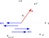Fig. 1. Reference frames S = {x,y,z} and S′={x′,y′,z′} are represented and the orientation of B and u are indicated for the uniform B configuration.

Let us consider first the DF of the perpendicular case of Paper I (Eq. (31) of Paper I) corresponding to the case Φ₀ = 0:

$$\begin{array}{c}\hfill f_{\perp }(x,v_x,v_y,v_z)=Cexp[-\frac{{\mathcal{E}}_0(x,v_x,v_y,v_z)}{m{v}_{th,p}^2}],\end{array}$$(13)

where ${\mathcal{E}}_0=\mathcal{E}-m{v}_{c\perp }^2/2$ is the “reduced” total energy where the kinetic energy associated with the guiding center motion has been subtracted, and v_c⊥ is the guiding center velocity component perpendicular to B (the only non-vanishing component in this case). C is a normalization constant and v_th, p is the proton thermal speed away from the shear region, where f_⊥ is reduced to an SM. The associated bulk velocity u_⊥ is also directed along the y′ direction (Paper I).

In the oblique case (Φ₀ ≠ 0), we want to obtain a bulk velocity u in the y direction, which has two components: u_⊥ and u_||, respectively, which are perpendicular and parallel to B. As in Paper I, the former component is due to the guiding center velocity v_c⊥ of particles. To obtain a parallel bulk velocity, u_||, as well, we add a shift U_|| of the DF in the velocity space along the v_z′ direction, similar to the shift that transforms a Maxwellian into an SM. This is coherent with the cyclicity of the z′ coordinate. The amount U_|| of the shift should (roughly) correspond to guiding centers moving along the y direction. The geometry suggests the relation U_||/v_c⊥ = tanΦ₀. On the basis of the above considerations, we modify the expression (13) and write the following form for the DF of uniform oblique B:

$$\begin{array}{c}\hfill f_{{\mathrm{\Phi }}_0}(x,\mathit{v})=Cexp\{-\frac{1}{2v_{\mathrm{th},\mathrm{p}}^2}[v_x^2+{\left[v_{y\prime }(v_y,v_z,{\mathrm{\Phi }}_0)\right]}^2\\ \hfill +{[v_{z\prime }(v_y,v_z,{\mathrm{\Phi }}_0)-v_{c\perp }(x,\mathit{v})tan{\mathrm{\Phi }}_0]}^2\\ \hfill +(2e/m)\varphi (x;x_c(x,\mathit{v}))-{\left[v_{c,\perp }(x,\mathit{v})\right]}^2]\},\end{array}$$(14)

where v_y′(v_y, v_z, Φ₀) = v_y cos Φ₀ − v_z sin Φ₀, v_z′(v_y, v_z, Φ₀) = v_y sin Φ₀ + v_z cos Φ₀, and v_c, ⊥(x, v) is the guiding center velocity of a particle that at a given time is at position x with velocity v (the knowledge of x and v fully determines the particle motion). The particular dependence of the DF (14) on the parallel drift velocity component v_z′ allows us to counterbalance the z component of the averaged gyrocenter velocity, thus obtaining a bulk velocity nearly aligned with the y direction. We observe that the form (14) for Φ₀ = 0 is reduced to the distribution function obtained in the case of “perpendicular B” (Eq. (31) of Paper I). It is important to note that the DF defined by Eq. (14) is expressed only in terms of constants of motion. In fact, the terms $v_x^2+v_{y^{\prime }}^2+(2e/m)\varphi (x;x_c)=2{\mathcal{E}}_{\perp }/m$, v_z′, and v_c⊥ are all constants of motions. Therefore, the DF (14) is a stationary solution of the Vlasov equation, provided that E and B remain stationary. This latter condition is to be subsequently verified.

The form (14) has been heuristically induced in the attempt to generalize the case considered in Paper I. Therefore, the associated bulk velocity, u, must be calculated a posteriori in order to verify to what extent it has the expected form. We also notice that the form (14) only implicitly defines the DF, because explicit expressions for the guiding center velocity v_c⊥(x, v) and position x_c(x, v) are not known for an arbitrary electric field profile E(x). Explicit analytical results will be obtained in the particular case of a linear profile for the electric field, denoted as a “local approximation”. In the general case, a numerical method will be applied to calculate the DF and its moments.

4.1. Local approximation

In the particular case of an electric field with a linear profile the single particle motion can be analytically calculated. In this case, the form (14) of the DF and of its moments can be explicitly written. In the following we briefly describe the main results of this case, while more details are given in Appendix A. The electric field has the form:

$$\begin{array}{c}\hfill E(x)=E_0+{\alpha }_0(x-x_0),\end{array}$$(15)

with E₀ and α₀ constant. Equation (15) can also be interpreted as a local first-order approximation of a general profile if |x − x₀| ≪ |E₀/α₀|. For ${\alpha }_0\ge m{\mathrm{\Omega }}_p^2/e$ particles moves along x linearly or exponentially in time, leading to a breakdown of the local approximation. Therefore, we consider only the case ${\alpha }_0<m{\mathrm{\Omega }}_p^2/e$, when the particle orbit in the velocity space is given by a shifted ellipse located in a plane parallel to the v_x′v_y′ plane, which is traveled with a gyrofrequency $\omega ={({\mathrm{\Omega }}_p^2-e{\alpha }_0/m)}^{1/2}$. The guiding center is the ellipse center (the explicit expression of x_c(x, v) is given in Appendix A); it moves with a transverse velocity that coincides with the E × B drift velocity calculated at the guiding center position: v_c⊥(x, v) = − cE(x_c)/B. A simple physical interpretation can be given to the condition ${\alpha }_0<m{\mathrm{\Omega }}_p^2/e$. In fact, such a condition corresponds to ΔF_e ≲ F_M, where ΔF_e = eα₀ρ ∼ eα₀v/Ω_p is the electric force variation across a length equal to the Larmor radius ρ, while v and F_M ∼ mvΩ_p are estimations of the particle velocity and of the magnetic force, respectively. Therefore, in the local approximation the particle trajectory is bounded provided that the magnetic force, responsible for the gyromotion, is large enough to hinder particle runaway due to F_e on a scale comparable with the Larmor radius. Using the expressions of x_c(x, v) and v_c⊥(x, v), the explicit form of the DF can be derived:

$$\begin{array}{cc}\hfill f_{{\mathrm{\Phi }}_0}^{(la)}(x,\mathit{v})& =\frac{n_0}{{(2\pi )}^{3/2}{v}_{\mathrm{th},\mathrm{p}}^3}\sqrt{\frac{{\mathrm{\Omega }}_p{B}_0}{{\mathrm{\Omega }}_p{B}_0-c{\alpha }_0}}exp\{-\frac{1}{2v_{\mathrm{th},\mathrm{p}}^2}\hfill \\ \hfill & \times \{v_x^2+\frac{{\mathrm{\Omega }}_p{B}_0}{{\mathrm{\Omega }}_p{B}_0-c{\alpha }_0}{[\frac{c{\alpha }_0}{B_0}(x-x_0)+v_{y\prime }-v_{d0}]}^2\hfill \\ \hfill & +[v_{z\prime }-v_{d0}tan{\mathrm{\Phi }}_0+\frac{c{\alpha }_{0}tan{\mathrm{\Phi }}_0}{{\mathrm{\Omega }}_p{B}_0-c{\alpha }_0}\hfill \\ \hfill & {\times [{\mathrm{\Omega }}_p(x-x_0)+v_{y\prime }-v_{d0}]]}^2\}\},\hfill \end{array}$$(16)

where n = n₀ is the uniform density and v_d0 = −cE₀/B₀ is the drift velocity at the position x₀. The associated bulk velocity takes the form:

$$\begin{array}{c}\hfill \mathit{u}\mathbf{(}\mathit{x}\mathbf{)}=-\frac{cE(x)}{B_0}{\mathit{e}}_{y\prime }-\frac{cE(x)}{B_0}tan{\mathrm{\Phi }}_0{\mathit{e}}_{z\prime }=-\frac{cE(x)}{B_{0}cos{\mathrm{\Phi }}_0}{\mathit{e}}_y.\end{array}$$(17)

The expression (17) corresponds to a planar shearing flow varying along x and directed at constant angle θ = π/2 − Φ₀ with B, at each x. Therefore, in the local approximation, the DF (14) reproduces the desired form for the bulk velocity exactly. In particular, the bulk velocity component, u_⊥ = u_y′, that is perpendicular to B is equal to the local E × B drift velocity.

4.2. General electric field profile

In the case of an electric field with a general profile, E(x), we used a numerical procedure to calculate the DF (14) and its moments. In the procedure, where the motion equations of single particles are integrated, the periodicity in the velocity space represents a key element. Of course, constants of motions appearing in expression (14) can be evaluated at any instant of time; therefore, the phase-space coordinates {x,v} are interpreted as the particle position and velocity at the initial time of its motion. In the numerical procedure, such initial conditions are taken on a regular grid in the phase-space (1D in the physical space and 3D in the velocity space): x(t = 0) = x_i, v_x(t = 0) = v_x, j, v_y(t = 0) = v_y, k, v_z(t = 0) = v_z, l (i, j, k, l are indexes that span on the 4D grid and identify the given particle). Starting from this set of initial conditions, the motion equations of each particle are integrated during one single period τ_ijkl. For the time integration, we used a third-order Adams-Bashforth scheme. Then the constants of motion were calculated: the guiding center transverse velocity v_{c ⊥ ,ijkl} = ⟨v_⊥⟩_τijkl and position x_c, ijkl = ⟨x⟩_τijkl, as well as the transverse energy $U_{\perp ,ijkl}=m(v_{y,k}^2+v_{z,l}^2)/2-e{\int }_{x_{c,ijkl}}^{x_i}E(x)dx$. Finally, these quantities, along with the parallel velocity v_z′,kl = v_y, k cos Φ₀ − v_z, l sin Φ₀, are inserted into expression (14) and the value of f_ϕ0(x_i, v_x, j, v_y, k, v_z, l) for the DF at the given phase-space point is calculated.

The set of values of the DF calculated on the grid points allow us to obtain the moments by numerically calculating the corresponding integrals. In particular, we found that the x component of the resulting bulk velocity is vanishing: u_x = 0, similar as in the local approximation (Eq. (17)). Therefore, the term u × B in the generalized Ohm’s law (3) is directed in the x direction. Moreover, in this configuration it is j = 0. Hence, only the x component of Eq. (3) is nonvanishing, which implies:

$$\begin{array}{c}\hfill \frac{\mathrm{d}{p}_e}{\mathrm{d}x}=-en(x)\{E(x)+\frac{B_0}{c}[u_y(x)cos{\mathrm{\Phi }}_0-u_z(x)sin{\mathrm{\Phi }}_0]\}.\end{array}$$(18)

This equation determines the electron pressure p_e(x).

Concerning the time dependence, let us assume that the obtained configuration holds at the initial time. Since ∂f_Φ0/∂t = 0, all the moments of f_Φ0 have a vanishing time derivative; in particular, it is ∂n/∂t = 0. Being ∇ × E = 0, the Faraday’s law (2) implies that ∂B/∂t = 0. Moreover, being (u ⋅ ∇)(p_e/n^γ_e) = 0, Eq. (4) implies ∂p_e/∂t = 0. Hence, from the Ohm’s law (3), it follows that ∂E/∂t = 0. We can conclude that the considered configuration is a stationary solution of the full set of HVM Eqs. (1)–(4).

4.3. Results for a double shear configuration

To illustrate our results, we consider a particular configuration with two opposite shear layers. We introduce rescaled variables: the magnetic field is normalized to B₀, time to ${\mathrm{\Omega }}_p^{-1}$, density to the value $\overline{n}$ away from the shear regions, velocities to the Alfvén velocity $v_A=B_0/{(4\pi m\overline{n})}^{1/2}$, lengths to the proton inertial length d_p = v_A/Ω_p, electric field to v_AB₀/c, and electron pressure to $\overline{n}m{v}_A^2$. To simplify the notation, in the remainder of this subsection, we denote rescaled quantities with the same symbols as the original quantities. In the homogeneous region, the proton plasma beta is $\beta =2v_{\text{th},\text{p}}^2/v_A^2=2$. We chose a spatial domain, D, defined by 0 ≤ x ≤ L, with L = 100 and the following form for the electric field:

$$\begin{array}{c}\hfill E(x)=E_0[1-tanh\left(\frac{x-L/4}{\mathrm{\Delta }x}\right)+tanh\left(\frac{x-3L/4}{\mathrm{\Delta }x}\right)],\end{array}$$(19)

where E₀ = cos Φ₀ and Δx = 2.5. This corresponds to two opposite shear layers of a width, Δx, located at x = L/4 and x = 3L/4, respectively. The proton thermal gyroradius in normalized units is ρ = v_th, p/Ω_p = 1, therefore, the shear width Δx is 2.5 larger than ρ. The electric field (19) is periodic in the domain D: E(0) = E(L)≃E₀, while in the center of the domain it is E(L/2)≃ − E₀. Moreover, E(x) vanishes in the limit Φ₀ → π/2, consistent with the case when B is parallel to u (Paper I). We calculated the DF (14) using the above-described procedure on a grid formed by N_x = 256 points in the x direction and N_v = 71 points in each velocity direction, v_i,  i = x, y, z, where −7v_th, p ≤ v_i ≤ 7v_th, p, with v_th, p = 1 (in scaled units). The $N_x{N}_v^3\simeq 9.16\times {10}^7$ particle trajectories have been calculated using a parallel computing procedure.

The associated density n(x) = ∫f_Φ0(x, v)d³v is plotted in Fig. 2 for cases when Φ₀ = π/6 and Φ₀ = π/3. In contrast with the local approximation, now the density, n(x), is not uniform, except away from the two shear regions. The non-uniformity of n(x) decreases with increasing Φ₀; actually, when B is parallel to u (corresponding to Φ₀ = π/2) the density profile is uniform (Paper I). In particular, n(x) is maximum (minimum) at the center of the shear at x = L/4 (x = 3L/4). This asymmetry between the two shear layers is a genuine kinetic effect that is related to the sign of the dot product (∇×u)⋅Ω_p, (Ω_p being the proton vector gyration angular velocity) which is opposite in the two shear layers.

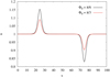Fig. 2. Profiles of density n(x) calculated for Φ0 = π/6 (black line) and Φ0 = π/3 (red line) in the uniform oblique B case.

The profiles of the bulk velocity components u_i(x) = ∫v_if_Φ0(x, v)d³v/n(x), i = y, z are plotted in Fig. 3 for Φ₀ = π/6. We notice that u is not exactly in the y direction, as in the local approximation case. However, |u_z| is about two orders of magnitude smaller than |u_y|, while |u_x|∼10⁻¹² (not shown). Therefore, the condition that u(x) and B form a constant angle θ = (π/2 − Φ₀) is well satisfied. The largest deviations from this condition are localized at the shear layers. Moreover, the profile of u_z(x) is qualitatively similar to −d²E(x)/dx²; this is not surprising, since for a linear electric field profile (15), it is u_z(x) = 0.

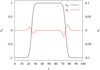Fig. 3. Profiles of bulk velocity components uy(x) (black line) and uz(x) (red line) calculated for Φ0 = π/6 in the uniform oblique B case. Different scales are used for uy and uz.

In the shear regions, the DF deviates from a Maxwellian. In particular, a temperature anisotropy develops that can be quantitatively evaluated by calculating the variance matrix. This has been done in the reference frame S′ where B is along the z′ axis. We refer to S′ as “local B frame” (LBF). The corresponding variance matrix is

$$\begin{array}{c}\hfill {\sigma }_{\mathit{ij}}^{\mathrm{LBF}}(x)=\frac{1}{n(x)}\int [v_i-u_i(x)][v_j-u_j(x)]f_{{\mathrm{\Phi }}_0}(x,\mathit{v})d^3\mathit{v},\end{array}$$(20)

with i, j = x′,y′,z′. Normalized parallel and perpendicular temperatures are given by $T_{||}={\sigma }_{z\prime z\prime }^{\mathrm{LBF}}$ and $T_{\perp }=({\sigma }_{x\prime x\prime }^{\mathit{LBF}}+{\sigma }_{y\prime y\prime }^{\mathit{LBF}})/2$, respectively, while the anisotropy and agyrotropy indexes are η^* = T_⊥/T_|| and ${\zeta }^{\ast }=min({\sigma }_{x\prime x\prime }^{\mathrm{LBF}},{\sigma }_{y\prime y\prime }^{\mathrm{LBF}})/max({\sigma }_{x\prime x\prime }^{\mathrm{LBF}},{\sigma }_{y\prime y\prime }^{\mathrm{LBF}})$, respectively (a gyrotropic DF corresponds to ζ^* = 1, otherwise it is ζ^* <  1). Since the variance matrix is symmetric, a reference frame exists (denoted as the minimum variance frame, MVF) where it is diagonal. Therefore, the eigenvalues λ⁽³⁾ <  λ⁽²⁾ <  λ⁽¹⁾ of σ_ij give the temperatures along the MVF axes. The corresponding anisotropy and agyrotropy indexes are defined by η = (λ⁽²⁾ + λ⁽³⁾)/(2λ⁽¹⁾) and ζ = λ⁽³⁾/λ⁽²⁾, respectively. In Fig. 4, the profiles of η, η^*, ζ, and ζ^* are plotted as functions of x, for Φ₀ = π/6. In the shear layers, the DF is both anisotropic and agyrotropic. Anisotropy is larger in the MVF than in the LBF in both shear layers. Agyrotropy is larger in the LBF than in the MVF in the shear layer at x = L/4, the reverse holds at x = 3L/4, owing to a different orientation between Ω_p and ∇ × u at each shear. A similar behavior holds also for ϕ₀ = π/3, except for a larger agyrotropy in the MVF in both shears (not shown).

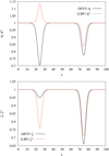Fig. 4. Upper panel: profiles of anisotropy parameters η (black line) and η* (red line); lower panel: profiles of agyrotropy parameters ζ (black line) and ζ* (red line). Both panels refer to Φ0 = π/6 in the uniform oblique B case.

Finally, we calculated the heat flux q, defined by

$$\begin{array}{c}\hfill \mathit{q}(x)=\frac{1}{2}\int [\mathit{v}-\mathit{u}(x)]{|[\mathit{v}-\mathit{u}(x)]|}^2{f}_{{\mathrm{\Phi }}_0}(x,\mathit{v})d^3\mathit{v}.\end{array}$$(21)

The components q_y and q_z are plotted in Fig. 5 as functions of x, for Φ₀ = π/6 and Φ₀ = π/3, while q_x is null for all x values. We see that q_y and q_z are not vanishing in the shear layers, where they have opposite behaviors. However, the average of both q_y and q_z across each shear layer is null.

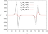Fig. 5. Profiles of heat flux components qy (black lines) and qz (red lines) for Φ0 = π/6 (full lines) and Φ0 = π/3 (dashed lines) in the uniform oblique B case.

4.4. Numerical simulation

Although the above-described configuration is, in principle, exactly stationary, since it has been derived through a numerical procedure it is necessarily affected by errors that arise during the time integration of single particle motion. Moreover, in the perspective of applying such results in numerical simulations, other errors would appear related to discretization in the phase space and time that is inherent to numerical codes. Therefore, it is interesting to study the time behavior of the above-described stationary state when it is used as initial condition in a HVM numerical simulation. This has the purpose to find a quantitative evaluation of departure from stationarity due to numerical errors.

A simulation was performed using a HVM numerical code, where periodic boundary conditions are applied in the physical space while it is assumed that the DF vanishes at the boundaries of the domain in the velocity space (|v_x, y, z|≥v_max = 7v_th, p). Details on the code can be found in Valentini et al. (2007). The simulation lasts up to the time t = 40 in normalized units. We calculated the time evolution of density and bulk velocity components, evaluating the departures from their initial profiles. In particular, for a given moment M(x, t), we calculated the corresponding L₂-norm departure with respect to the initial profile M(x, 0):

$$\begin{array}{c}\hfill L_2(\delta M)(t)={\left\{\frac{1}{L}{\int }_0^L{[M(x,t)-M(x,0)]}^{2}dx\right\}}^{1/2}.\end{array}$$(22)

In Fig. 6, the density L₂(δn) and bulk velocity L₂(δu_i) (i = x, y, z) departures are plotted as functions of t, as they result from the simulation. As expected, such departures do not remain null. However, after a fast increase lasting few time units, both L₂(δn) and L₂(δu_i) saturate at a level that has an order of magnitude between 10⁻⁴ and 10⁻³. In Fig. 7 the profiles u_y(x) calculated at the initial and at the final time are plotted. The two profiles are practically superimposed; therefore, the width of shear layers remains essentially unchanged during the considered time evolution. To visualize variations of the profile u_y(x) during the time evolution; in the same figure, we superimposed the difference, Δu_y(x) = u_y(x, t = 40)−u_y(x, t = 0) (using a different scale). It can be seen that max|Δu_y| is of the order of 0.001 and variations are essentially confined within the two shear layers. We conclude that numerical errors affect the stationarity of the solution to a low extent.

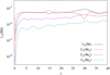Fig. 6. Profiles of L2(δn) (black line), L2(δux) (red line), L2(δuy) (purple line), and L2(δuz) (green line) as functions of time, as they result from the HVM simulation.

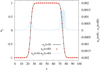Fig. 7. Profiles of uy(x) calculated at the initial (black solid line) and final (red balls) time of the simulation. The difference between the two curves Δuy is also plotted (blue solid line).

5. B with uniform intensity and variable direction

The second configuration, corresponds to a nonuniform magnetic field, B, whose direction changes in space, but keeping |B| uniform. This kind of configuration is more realistic for the magnetopause than the previous case where B had a constant direction. In fact, in many circumstances the magnetic field direction on the solar wind side is different from that on the magnetosphere side (see, e.g., Faganello & Califano 2017). The present case corresponds to a configuration described by Eq. (5), where the angle Φ(x) between B(x) and the z-axis is not constant. In this case, particle trajectories are not planar curves.

To have an indication to how to find an appropriate stationary solution, we first examined a local approximation. We consider electric and magnetic field varying linearly with x, assuming the form (15) for E(x) and the equations:

$$\begin{array}{c}\hfill B_y(x)=B_0[b_{0y}+{\gamma }_y(x-x_0)],\end{array}$$(23)

$$\begin{array}{c}\hfill B_z(x)=B_0[b_{0z}-{\gamma }_z(x-x_0)],\end{array}$$(24)

where b_0y, 0z and γ_y, z are constants and |x − x₀| ≪ |b_0y, 0z/γ_y, z|. In studying the particle dynamics, all terms that are quadratic or of higher order in the ratios |γ_y, z(x − x₀)/b_0y, 0z| will be neglected. Here, we give only the main results of the procedure, while details can be found in the Appendix B. The particle motion along x corresponds to a harmonic oscillator x(t) = R₀sin(ωt + φ)+x_c, where the R₀ is amplitude, φ is the phase, the frequency is

$$\begin{array}{c}\hfill \omega ={[{\mathrm{\Omega }}_p^2+{\mathrm{\Omega }}_p(w_y{\gamma }_z+w_z{\gamma }_y)-\frac{e{\alpha }_0}{m}]}^{1/2},\end{array}$$(25)

and x_c is the center of the oscillation, corresponding to the guiding center position (the expression of x_c is given in Appendix B). This solution holds if ${\alpha }_0<(m/e)\left[{\mathrm{\Omega }}_p^2+{\mathrm{\Omega }}_p\left(w_y{\gamma }_z+w_z{\gamma }_y\right)\right]$, otherwise the local approximation breaks down. Coordinates y(t) and z(t) can be calculated using the Eq. (7). Due to the quadratic form of a_y(x) and a_z(x), the coordinates y(t) and z(t) as well as the velocity components v_y(t) and v_z(t) are no longer harmonic functions of time. This implies that the closed trajectory in the velocity space is not an ellipse, as in the previous configuration and, in general, it is not planar. However, the following simple relation holds for the components v_cy = ⟨v_y⟩ and v_cz = ⟨v_z⟩ of the guiding center velocity: v_czB_y(x_c)−v_cyB_z(x_c) = cE(x_c), which implies that the guiding center velocity component perpendicular to B(x_c) is equal to the local E × B drift velocity:

$$\begin{array}{c}\hfill v_{c\perp }=c\frac{\mathit{E}(x_c)\times \mathit{B}(x_c)}{B_0^2}.\end{array}$$(26)

This same property of the guiding center velocity was found in the oblique B configuration. This analogy will be exploited to generalize the DF found in the case of oblique uniform B to the present case of non-uniform B. For this purpose, we go back to the uniform-B case and re-write the argument of the exponential in Eq. (14) (valid in the former case) in the following form:

$$\begin{array}{c}\hfill F_{{\mathrm{\Phi }}_0}=-\frac{2\mathcal{E}/m-v_{z\prime }^2+{(v_{z\prime }-v_{c\perp }tan{\mathrm{\Phi }}_0)}^2-v_{c\perp }^2}{2v_{\mathrm{th},\mathrm{p}}^2}.\end{array}$$(27)

The velocity component v_z′ in this expression can be interpreted as the guiding center velocity component parallel to B: v_z′ = v_c||. Therefore, we write

$$\begin{array}{c}\hfill F_{{\mathrm{\Phi }}_0}=-\frac{2\mathcal{E}/m-v_{c||}^2+{[v_{c||}-U_{||}(v_{c\perp })]}^2-v_{c\perp }^2}{2v_{\mathrm{th},\mathrm{p}}^2},\end{array}$$(28)

where U_||(v_c⊥) = v_c⊥tanΦ₀. Expression (28) is valid in any reference frame and, therefore, it is suitable to be generalized as per the nonuniform-B case. Indeed, to obtain such a generalization, we have only to specify another form for the function U_||(v_c⊥), which has the role of generating a bulk velocity component parallel to B. In the case of nonuniform B, the magnetic field changes direction with x while the bulk velocity u must keep parallel to the y axis for any x. Indicating by e_|| = B/B and e_⊥ = e_|| × e_x the unit vectors parallel and perpendicular to B, we can assume that u ∼ U_||e_|| + v_c⊥e_⊥. Imposing u_z = 0 in the previous expression we derive the relation U_|| = (B_y/B_z)v_c⊥ = v_c⊥tanΦ. On the base of the above considerations, we assume the following form for the DF in the general case:

$$\begin{array}{cc}\hfill f_{\mathrm{\Phi }(x)}(x,\mathit{v})& =Cexp\{-\frac{1}{2v_{\mathrm{th},\mathrm{p}}^2}\{v_x^2+v_y^2+v_z^2+\hfill \\ \hfill & (2e/m)\varphi (x;x_c(x,\mathit{v}))-{\left[v_{c||}(x,\mathit{v})\right]}^2-{\left[v_{c\perp }(x,\mathit{v})\right]}^2\hfill \\ \hfill & +{[v_{c||}(x,\mathit{v})-v_{c\perp }(x,\mathit{v})tan\mathrm{\Phi }(x_c(x,\mathit{v}))]}^2\}\}.\hfill \end{array}$$(29)

The associated electron pressure, p_e, is calculated by Eq. (4). We show that the bulk velocity component u_x is vanishing; moreover, it is j × B = 0. Therefore, the only nonvanishing component of Eq. (4) is reduced to

$$\begin{array}{c}\hfill \frac{\mathrm{d}{p}_{\mathrm{e}}}{\mathrm{d}x}=-en(x)\{E(x)+\frac{B_0}{c}[u_y(x)cos\mathrm{\Phi }(x)\\ \hfill -u_z(x)sin\mathrm{\Phi }(x)]\},\end{array}$$(30)

which determines the profile p_e(x).

We observe that f_Φ(x)(x, v) is expressed only in terms of the constants of motion: total energy, ℰ, guiding center position, x_c, and velocity, v_c. Therefore, the DF (29) is a stationary solution of the Vlasov Eq. (1), provided that the electric and magnetic field remain constant in time. Indeed, using the same arguments as in the case of uniform B, it can be shown that ∂E/∂t = ∂B/∂t = ∂p_e/∂t = 0. We conclude that the considered configuration is a stationary solution of the whole set of Eqs. (1)–(4). We also note that expression (29) is reduced to the form (14) when Φ(x) = Φ₀ = const.

For general profiles of E(x) and Φ(x), an explicit evaluation of the DF (29) can be obtained using the same numerical procedure as in the case when Φ(x) = Φ₀ = const, which determines f_Φ(x) on a 4D grid in the {x,v} phase space. In particular, for the sake of illustration we consider a particular case where E(x) is given by Eq. (19) and

$$\begin{array}{c}\hfill \mathrm{\Phi }(x)=\mathrm{\Delta }\mathrm{\Phi }[tanh\left(\frac{x-L/4}{\mathrm{\Delta }x}\right)-tanh\left(\frac{x-3L/4}{\mathrm{\Delta }x}\right)-1].\end{array}$$(31)

In this configuration, B rotates by an angle ±2ΔΦ across the shear layers, while it is essentially uniform away from the shear layers. The B_y component changes sign across the shear layers, while B is in the z direction at the center of each shear layer, x = L/4 and x = 3L/4, where Φ = 0. The width Δx of the magnetic shears is the same as that of the velocity shears.

Numerical results are presented for L = 100, Δx = 2.5 (in normalized units) and for various values of ΔΦ. In Fig. 8, we plot the trajectory of a particle in the velocity space. The curve is more complex than those typically found in the case of uniform B and is not planar. We have calculated the moments of the DF (29) for this configuration. In Fig. 9, the density profile n(x) is plotted; as for the uniform-B case, n(x) has a local maximum or minimum at shear layers, according to the sign of (∇×u)⋅Ω_p at shear layers. This asymmetry tends to increase and the profile n(x) becomes more complex for increasing ΔΦ. For all the values of ΔΦ, the DF has been normalized by imposing that ${\int }_0^{L}n(x)\text{d}x/L=1$.

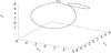Fig. 8. Trajectory in the velocity space of a particle starting from x = 75, vx = −1, vy = 0.5, vz = 6.5.

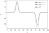Fig. 9. Profiles of density n as a function of x calculated for ΔΦ = π/6 (black line), ΔΦ = π/4 (blue line), and ΔΦ = π/3 (red line) in the case of nonuniform B.

In Fig. 10, the profiles of the bulk velocity components u_y(x) and u_z(x) are plotted, using different scales for the two profiles (u_x is vanishing). The bulk velocity is not exactly aligned along y; however, it is |u_z(x)| ≪ |u_y(x)|. Therefore, the desired condition that u is along the same direction in the whole domain is reasonably well satisfied by the DF (29). In Fig. 11, the anisotropy η, η^* and agyrotropy ζ, ζ^* parameters are plotted in the case ΔΦ = π/4. The DF is anisotropic and agyrotropic at the shear layers, with respect to both the MVF and LBF. The profiles of heat flux components q_y and q_z are plotted in Fig. 12 in the case ΔΦ = π/4 (it is q_x = 0). A peculiar feature is that the q_z component averaged across one shear layer ⟨q_z⟩_sl is no longer vanishing; this holds for both shear layers where a net heat flux directed opposite to the mean magnetic field ⟨B⟩_sl has been found. A similar behaviour has been found also for other values of ΔΦ (not shown). Finally, in Fig. 13, 3D contour plots of the DF in the velocity space are plotted at three different positions across one shear layer. Blue arrows indicate the local direction of B. Lack of both isotropy and gyrotropy is clearly visible. Moreover, in the position x = L/4 corresponding to the shear layer center (middle panel), an asymmetry with respect to the exchange v_z ⇌ ( − v_z) is evident. Such a feature is responsible for the net heat flux in the −z direction.

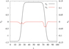Fig. 10. Profiles of bulk velocity components uy (black line) and uz (red line) as functions of x calculated for ΔΦ = π/4 in the case of nonuniform B. Different scales are used for uy and uz.

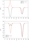Fig. 11. Upper panel: profiles of anisotropy parameters η (black line) and η* (red line); lower panel: profiles of agyrotropy parameters ζ (black line) and ζ* (red line). Both panels refer to ΔΦ = π/4 in the nonuniform B case.

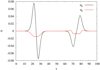Fig. 12. Profiles of heat flux components qy (black line) and qz (red line) are plotted as functions of x, calculated for ΔΦ = π/4 in the case of nonuniform B.

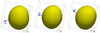Fig. 13. Iso-surface plots of proton DFs in three different positions along the x-axis: x = L/4 − 2.34 (left panel),x = L/4 (middle panel), x = L/4 + 2.34 (right panel). The blue arrow indicates the direction of the background magnetic field (B0).

6. Conclusions

In this paper, we derive exact solutions for the system of HVM equations representing a stationary shearing flow in collisionless magnetized plasmas. In many natural contexts, there are configurations where a plasma is characterized by shearing flows. A kinetic description is necessary whenever the shear width is of the order of kinetics scales, as, for instance, in the case of Earth’s magnetophause (Sckopke et al. 1981; Kivelson & Chen 1995; Faganello & Califano 2017).

The interest of building up stationary solutions can be related to the problem of describing the propagation and evolution of waves in a plasma with a stable shearing flow. The interaction between waves and the background inhomogeneity associated with the shearing flow moves the wave energy toward small scales, where kinetic effects are more effective. Moreover, the presence of a shearing flow can generate wave coupling, with an energy transfer among different wave modes. It is clear that in order to properly study wave propagation, it is necessary for the background structure to remain stationary; otherwise, a time evolution intrinsic of the background state would superpose onto the waves, making it difficult to single out the wave contribution in the overall time evolution. Another possible application of exact shearing flow solutions can be found in the study of KHI, which takes place in unstable shearing velocity configurations. In fact, only a stationary, unperturbed configuration allows us to properly describe both linear and nonlinear stages of the instability, as shown by Settino et al. (2020). Therefore, in both cases, it is crucial to use an exact stationary distribution function.

Stationary solutions in various configurations have been derived in previous studies of the fully kinetic case, that is, involving the full set of ion and electron Vlasov-Maxwell equations (Ganguli et al. 1988; Nishikawa et al. 1988; Cai et al. 1990; Mahajan & Hazeltine 2000). Allanson et al. (2016) have studied stationary DFs as products of a Maxwellian multiplied by a combination of Hermite expansions depending on canonical momenta that are constants of motions. Similarly, our most general expression (29) can be factorized as a product of a Maxwellian by a factor that is dependent only on constants of motions. However, our approach presents several differences with respect to that of Allanson et al. (2016). First, our results are relative to the HVM theory, while in the approach by Allanson et al., ions and electrons are both kinetically represented. Moreover, in our case, charge neutrality is only approximately satisfied and an electric field is present that is responsible for plasma drift motion. In contrast, Allanson et al. (2016) consider perfect charge neutrality and null electric field, while the method is applied to calculate equilibria without a bulk velocity. The fully kinetic treatment is quite complex and such solutions have rarely been employed in numerical simulations as, for instance, in investigations of KHI. In this respect, the set of HVM equations represents a good compromise because it correctly describes a plasma at scales of the order of or larger than ion scales but while avoiding the complexity of a fully kinetic treatment.

Within this framework, the exact stationary solutions of Paper I have been set into the special cases where the magnetic field is uniform and either parallel or perpendicular to the bulk velocity. In the present paper, we extend these previous results to more general magnetized shearing flow configurations, namely: (1) uniform obliquely-directed magnetic field; and (2) variable-directed uniform-intensity magnetic field. In the first configuration, the magnetic field, B, is uniform and forms a constant angle with the bulk velocity, u. In the second configuration the angle between B and u is not constant and changes along the direction perpendicular to u and B. Such configurations are more general than those considered in Paper I and they can more realistically represent the magnetic configuration across the magnetopause (e.g., Faganello & Califano 2017). Therefore, they can be employed as a background state in future studies of KHI in the magnetopause in various magnetic configurations, as we are planning to do.

Stationary DFs have been built up as appropriate combinations of single-particle constants of motions, that have been derived through successive generalizations of those found in Paper I. Stationarity with respect to the whole set of HVM equations has been verified. Explicit analytical forms for the DFs has been derived within the local approximation where both E(x) and B(x) have linear profiles. For more general profiles, a numerical procedure has been set up to integrate single-particle motion, to calculate the corresponding values of involved constants of motions, and to derive the DF on a grid in the phase space. We characterize our results by calculating profiles of moments such as density, bulk velocity, and heat flux. Solving the extended two-fluid model equations, Cerri et al. (2013) found that, starting from an MHD equilibrium with uniform density, the density profile tends to a shape qualitatively similar to that shown in Figs. 2 and 9; namely, a maximum and a minimum located at the shear layer where (∇×u)⋅Ω_p is negative or positive, respectively. However, the amplitude of density variation is ∼3 − 4% in Cerri et al. (2013), while it is ∼10 − 15% in our case. This discrepancy could be partially due to a slightly different shear width (Δx = 3 in Cerri et al. 2013, Δx = 2.5 in our case) and to the fact that the extended two-fluid model is not exactly equivalent to the HVM model.

We also calculated quantities quantifying departures of the DF from Maxwellianity. In particular, we found that in the shear layers, the DF is characterized by a marked anisotropy and agyrotropy. A peculiar property found in the shear regions is a net heat flux in the direction antiparallel to the mean B due to an asymmetry of the DF. We also verified that the obtained bulk velocity presents the desired orientation and planarity to a very good extent in both cases. A numerical simulation performed by means of the HVM code has allowed us to verify that departures from stationarity due to numerical errors remain at a low level, at least in the uniform B case. In particular, the width Δx of both shear layers remains essentially unchanged. This aspect is particularly relevant in the perspective of using the present stationary solutions to study the KHI. In fact, the growth rate as well as the wavelength of the fastest growing mode are affected by the value of the shear layer width, Δx. For instance, Nakamura et al. (2010) and Henri et al. (2013) showed that initializing a kinetic code with a shifted Maxwellian not only produces spurious oscillations but also a widening or thinning of the shear layer, depending on the relative orientation of ∇ × u and B. Our solution should allow future studies to overcome such a problem.

Further possible developments of the present work that we are planning to carry out involve the inclusion of inhomogeneities of magnetic field intensity |B|. This would allow us to perform a further step towards a more realistic representation of configurations, such as those found around the magnetopause. We also plan to use the configurations considered here to simulate the development of KHI in situations where kinetic effects at ion scales can play an important role.

Acknowledgments

Numerical simulations have been run on Marconi supercomputer at CINECA (Italy) within the ISCRA projects: IsC68_TURB-KHI and IsB19_6DVLAIDA. This work has received funding from the European Unions Horizon 2020 research and innovation programme under grant agreement no. 776262 (AIDA, www.aida-space.eu).

References

Appendix A: Local approximation for uniform oblique B

In this appendix, we focus a more detailed study on a configuration where the electric field has the linear profile of (15), which can be considered as a local approximation for a general profile E(x) around the position x₀. In particular, we derive the expressions for the guiding center velocity and for the DF (Eq. (16)). The form for the magnetic field is given by Eq. (5) with Φ(x) = Φ₀ = const. With respect to the reference frame S′, the normalized vector potential has the form a(x) = xe_y′. In this case, Eq. (8) becomes d²x/dt² + ω²x = (e/m)(E₀−α₀x₀) + Ω_pw_y′ where ${\omega }^2={\mathrm{\Omega }}_p^2-e{\alpha }_0/m$ and $w_{y^{\prime }}=v_{y^{\prime }}+{\mathrm{\Omega }}_{p}x$ is a constant of motion. If ${\alpha }_0<m{\mathrm{\Omega }}_p^2/m$, the above equation describes an harmonic oscillator of solution

$$\begin{array}{c}\hfill x(t)=R_{0}sin(\omega t+\phi )+x_c,\end{array}$$(A.1)

where R₀ and φ are the amplitude and the phase of the oscillation.

The guiding center position is given by the constant term:

$$\begin{array}{c}\hfill x_c={⟨x⟩}_{\tau }=\frac{1}{{\omega }^2}[\frac{e}{m}(E_0-{\alpha }_0{x}_0)+{\mathrm{\Omega }}_p{w}_{y\prime }],\end{array}$$(A.2)

that can be expressed as a function of x and v_y′:

$$\begin{array}{c}\hfill x_c=\frac{1}{1-c{\alpha }_0/({\mathrm{\Omega }}_p{B}_0)}[x-\frac{v_{y\prime }}{{\mathrm{\Omega }}_p}+\frac{c}{{\mathrm{\Omega }}_p{B}_0}(E_0-{\alpha }_0{x}_0)].\end{array}$$(A.3)

The velocity components are given by

$$\begin{array}{c}\hfill v_x(t)=R_0\omega cos(\omega t+\phi ),\end{array}$$(A.4)

$$\begin{array}{c}\hfill v_{y\prime }(t)=-{\mathrm{\Omega }}_{p}x(t)+w_{y\prime }=-R_0{\mathrm{\Omega }}_{p}sin(\omega t+\phi )+v_{c\perp },\end{array}$$(A.5)

and v_z′(t) = const, where v_c⊥ = ⟨v_y′(t)⟩_τ = −Ω_px_c + w_y′. By inserting Eq. (A.2) into this expression, we obtain v_c⊥ = −[e/(mω²)](Ω_pE₀+α₀v_0y′), where v_0y′ = −Ω_px₀ + w_y′ is the value of v_y′ at the position x₀. On the other hand, with w_y′ as a constant of motion, it is v_0y′ = v_c⊥ + Ω_p(x_c − x₀) (see Eq. (7)). Using this relation, from the above equations, we derive:

$$\begin{array}{c}\hfill v_{c\perp }=-\frac{e}{m\omega }[E_0+{\alpha }_0(x_c-x_0)]=-c\frac{E(x_c)}{B_0},\end{array}$$(A.6)

indicating that the guiding center velocity component perpendicular to B is given by the E × B drift velocity calculated at the guiding center position x_c.

The argument of the exponential in Eq. (14) contains the constant of motion $2{\mathcal{E}}_{\perp }/m-v_{c\perp }^2=v_x^2+v_{y^{\prime }}^2+(2e/m)\varphi -v_{c\perp }^2$. Such a constant can be evaluated at x = x_c, where the potential is ϕ = 0; at that position, it is sin(ωt + φ) = 0 and then v_x(x = x_c) = ± R₀ω and v_y′(x = x_c) = v_c⊥ (see Eqs. (A.4) and (A.5)). As a consequence, it is $2{\mathcal{E}}_{\perp }/m-v_{c\perp }^2=R_0^2{\omega }^2$ and, thus, Eq. (14) can be written as:

$$\begin{array}{c}\hfill f_{{\mathrm{\Phi }}_0}^{\mathit{la}}=Cexp[-\frac{R_0^2{\omega }^2+{(v_{z\prime }-v_{c\perp }tan{\mathrm{\Phi }}_0)}^2}{2v_{\mathrm{th},\mathrm{p}}^2}].\end{array}$$(A.7)

Using Eqs. (A.4), (A.5), and (A.6), the constant $R_0^2{\omega }^2$ can be expressed as a function of x , v_x and v_y′ in the following form:

$$\begin{array}{c}\hfill R_0^2{\omega }^2=v_x^2+\frac{{\omega }^2}{{({\mathrm{\Omega }}_p-c{\alpha }_0/B_0)}^2}{(v_{y\prime }+\frac{cE(x)}{B_0})}^2.\end{array}$$(A.8)

From Eqs. (A.6) and (A.3), we can express v_c⊥ as a function of x and v_y′:

$$\begin{array}{c}\hfill v_{c\perp }=v_{d0}-\frac{c{\alpha }_0}{{\mathrm{\Omega }}_p{B}_0-c{\alpha }_0}[{\mathrm{\Omega }}_p(x-x_0)+v_y-v_{d0}],\end{array}$$(A.9)

where v_d0 = −cE₀/B₀ is the drift velocity at the position x₀. By inserting Eqs. (A.8) and (A.9) into Eq. (A.7), this can be manipulated and, finally, written in the form of (16), where the normalization constant C has been determined by imposing $\int f_{{\Phi }_0}^{la}{d}^3\mathit{v}=n_0$. A straightforward calculation allows us to find Eq. (17).

Appendix B: Local approximation for uniform-intensity variable-direction B

In this appendix, we derive the form for the DF in the case of the local approximation for a magnetic field with uniform intensity and variable direction. The electric field takes the form of Eq. (15) and the magnetic field components have linear profiles given by Eqs. (23) and (24), where x₀ represents the center of the Taylor expansion. The corresponding potentials are

$$\begin{array}{c}\hfill \varphi (x)=-E_0(x-x_0)-\frac{{\alpha }_0}{2}{(x-x_0)}^2+{\varphi }_0,\end{array}$$(B.1)

$$\begin{array}{c}\hfill a_y(x)=b_{0z}(x-x_0)-\frac{{\gamma }_z}{2}{(x-x_0)}^2,a_z(x)=-b_{0y}(x-x_0)-\frac{{\gamma }_y}{2}{(x-x_0)}^2,\end{array}$$(B.2)

with ϕ₀ = const. Imposing the |B(x)| = B₀ = uniform, at the linear order we obtain the relations:

$$\begin{array}{c}\hfill b_{0y}^2+b_{0z}^2=1,b_{0y}{\gamma }_y=b_{0z}{\gamma }_z.\end{array}$$(B.3)

In coherence with the local approximation, in what follows, we neglect all terms cubic or of higher order in the ratios |α₀(x − x₀)/E₀| and |γ_y, z(x − x₀)/b_0y, 0z|. The single particle equation of motion in the x direction takes the form d²x/dt² + ω²x = (e/m)(E₀ − α₀x₀)+Ω_pW₀, where ω is given by Eq. (25) and

$$\begin{array}{c}\hfill W_0=(w_y{\gamma }_z+w_z{\gamma }_y)x_0+w_y{b}_{0z}-w_z{b}_{0y}+{\mathrm{\Omega }}_p{x}_0.\end{array}$$(B.4)

If ${\alpha }_0<(m/e)\left[{\mathrm{\Omega }}_p^2+{\mathrm{\Omega }}_p\left(w_y{\gamma }_z+w_z{\gamma }_y\right)\right]$ it is ω² >  0 and the particle motion along x is that of an harmonic oscillator,

$$\begin{array}{c}\hfill x(t)=R_{0}sin(\omega t+\phi )+x_c,v_x(t)=R_0\omega cos(\omega t+\phi ),\end{array}$$(B.5)

where R₀ is the amplitude, φ is the phase and x_c is the center of motion,

$$\begin{array}{cc}& x_c=\frac{1}{{\omega }^2}\{\frac{e}{m}(E_0+{\alpha }_0{x}_0)+\hfill \\ \hfill & +{\mathrm{\Omega }}_p[w_y(b_{0z}+{\gamma }_z{x}_0)-w_z(b_{0y}-{\gamma }_y{x}_0)+\mathrm{\Omega }{x}_0]\},\hfill \end{array}$$(B.6)

corresponding to the x position of the guiding center. Otherwise, if ${\alpha }_0\ge (m/e)\left[{\mathrm{\Omega }}_p^2+{\mathrm{\Omega }}_p\left(w_y{\gamma }_z+w_z{\gamma }_y\right)\right]$ the motion along x is not bounded and the local approximation breaks down. On the other hand, the motion equation along x can be re-written in the form dv_x(t)/dt = (e/m)E(x(t)) + Ω_p{v_y[da_y(x(t))/dx]+v_z[da_z(x(t))/dx]}. By inserting Eq. (B.5) into both sides and neglecting third-order terms, we obtain the following relation:

$$\begin{array}{c}\hfill -cE(x_c)=w_y{B}_z(x_c)-w_z{B}_y(x_c)-{\mathrm{\Omega }}_p{B}_0(x_c-x_0).\end{array}$$(B.7)

Using Eqs. (7), (B.2), and (B.5), we derive expressions for v_y and v_z:

$$\begin{array}{c}\hfill v_y(t)=w_y-{\mathrm{\Omega }}_p{a}_y(x_c)-\frac{{\mathrm{\Omega }}_p{B}_z(x_c)}{B_0}{R}_{0}sin(\omega t+\phi )+\frac{{\mathrm{\Omega }}_p{\gamma }_z}{2}{R}_0^2{sin}^2(\omega t+\phi ),\end{array}$$(B.8)

$$\begin{array}{c}\hfill v_z(t)=w_z-{\mathrm{\Omega }}_p{a}_z(x_c)+\frac{{\mathrm{\Omega }}_p{B}_y(x_c)}{B_0}{R}_{0}sin(\omega t+\phi )+\frac{{\mathrm{\Omega }}_p{\gamma }_y}{2}{R}_0^2{sin}^2(\omega t+\phi ).\end{array}$$(B.9)

We observe that, as a consequence of the dependence on sin²(ωt + φ) in v_y(t) and v_z(t), particle trajectories in the velocity space are no longer ellipses but have a more complex form. The y and z components of the guiding center velocity are

$$\begin{array}{c}\hfill v_{\mathit{cy}}={⟨v_y⟩}_{\tau }=\frac{{\mathrm{\Omega }}_p{\gamma }_z}{2}{(x_c-x_0)}^2-{\mathrm{\Omega }}_p{b}_{0z}(x_c-x_0)+\frac{{\mathrm{\Omega }}_p{R}_0^2{\gamma }_z}{4}+w_y,\end{array}$$(B.10)

References

- Allanson, O., Neukirch, T., Troscheit, S., & Wilson, F. 2016, J. Plasma Phys., 82, 905820306 [CrossRef] [Google Scholar]
- Axford, W. I. 1960, QJMAM, 8, 314 [Google Scholar]
- Bruno, R., & Carbone, V. 2013, Liv. Rev. Sol. Phys., 10, 2 [Google Scholar]
- Cai, D., Storey, L. R. O., & Neubert, T. 1990, PhFlB, 2, 75 [Google Scholar]
- Califano, F., Chiuderi, C., & Einaudi, G. 1990, ApJ, 365, 757 [NASA ADS] [CrossRef] [Google Scholar]
- Califano, F., Chiuderi, C., & Einaudi, G. 1992, ApJ, 390, 560 [NASA ADS] [CrossRef] [Google Scholar]
- Cerri, S. S., Henri, P., Califano, F., et al. 2013, Phys. Plasmas, 20, 112112 [NASA ADS] [CrossRef] [Google Scholar]
- Cerri, S. S., Pegoraro, F., Califano, F., Del Sarto, D., & Jenko, F. 2014, PhPl, 21, 112109 [CrossRef] [Google Scholar]
- Cerri, S. S., Califano, F., Jenko, F., Told, D., & Rincon, F. 2016, ApJ, 822, L12 [CrossRef] [Google Scholar]
- Cerri, S. S., Servidio, S., & Califano, F. 2017, ApJ, 846, L18 [CrossRef] [Google Scholar]
- Chandrasekhar, S. 1961, Hydrodynamic and Hydromagnetic Stability (Oxford University Press) [Google Scholar]
- Contin, J. E., Gratton, F. T., & Farrugia, C. J. 2003, JGRA, 108, 1227 [CrossRef] [Google Scholar]
- Cowee, M. M., & Winske, D., & Gary, S. P., 2009, JGRA, 4, A10209 [Google Scholar]
- Del Sarto, D., Pegoraro, F., & Califano, F. 2016, PhRvE, 93, 053203 [Google Scholar]
- Eriksson, S., Lavraud, B., Wilder, F. D., et al. 2016, GeoRL, 43, 5606 [Google Scholar]
- Ershkovich, A. I., & Mendis, D. A. 1983, ApJ, 269, 743 [CrossRef] [Google Scholar]
- Faganello, M., & Califano, F. 2017, JPlPh, 83, 535830601 [Google Scholar]
- Faganello, M., Califano, F., & Pegoraro, F. 2008, PhRvL, 100, 015001 [Google Scholar]
- Fairfield, D. H., Otto, A., Mukai, T., et al. 2000, JGRA, 105, 21159 [CrossRef] [Google Scholar]
- Fairfield, D. H., Farrugia, C. J., Mukai, T., Nagai, T., & Fedorov, A. 2003, JGRA, 108, 1460 [CrossRef] [Google Scholar]
- Foullon, C., Verwichtel, E., Nakariakov, V. M., Nykyri, K., & Farrugia, C. J. 2011, ApJ, 729, L8 [NASA ADS] [CrossRef] [Google Scholar]
- Franci, L., Verdini, A., Matteini, L., Landi, S., & Hellinger, P. 2015, ApJ, 804, L39 [NASA ADS] [CrossRef] [Google Scholar]
- Fujimoto, M., Terasawa, T., Mukai, T., et al. 1998, J. Geophys. Res., 103, 4391 [CrossRef] [Google Scholar]
- Ganguli, G., Lee, Y. C., & Palmadesso, P. J. 1988, PhFl, 31, 823 [Google Scholar]
- Hamlin, N. D., & Newman, W. I. 2013, Phys. Rev. E, 87, 043101 [NASA ADS] [CrossRef] [Google Scholar]
- Hasegawa, H., Fujimoto, M., Phan, T.-D., et al. 2004, Nature, 430, 755 [NASA ADS] [CrossRef] [Google Scholar]
- Hasegawa, H., Fujimoto, M., Takagi, K., et al. 2006, JGRA, 111, 9203 [CrossRef] [Google Scholar]
- Henri, P., Cerri, S. S., Califano, F., et al. 2013, PhPl, 20, 102118 [CrossRef] [Google Scholar]
- Hollweg, J. V. 1987, ApJ, 312, 880 [NASA ADS] [CrossRef] [Google Scholar]
- Kaghashvili, E. K. 1999, ApJ, 512, 969 [NASA ADS] [CrossRef] [Google Scholar]
- Kaghashvili, E. K., Raeder, J., Webb, G. M., & Zank, G. P. 2006, Phys. Plasmas, 13, 112107 [CrossRef] [Google Scholar]
- Kaghashvili, E. K. 2007, Phys. Plasmas, 14, 044502 [CrossRef] [Google Scholar]
- Karimabadi, H., Roytershteyn, V., Wan, M., et al. 2013, JPlPh, 20, 012303 [Google Scholar]
- Kivelson, M. G., & Chen, S. 1995, in Physics of the Magnetopause (Washington, DC: AGU), Geophys. Monogr. Ser., 90 [Google Scholar]
- Landi, S., Velli, M., & Einaudi, G. 2005, ApJ, 624, 392 [NASA ADS] [CrossRef] [Google Scholar]
- Lee, M., & Roberts, B. 1986, ApJ, 301, 430 [NASA ADS] [CrossRef] [Google Scholar]
- Mahajan, S. M., & Hazeltine, R. D. 2000, PhPl, 7, 1287 [CrossRef] [Google Scholar]
- Maiorano, T., Settino, A., Malara, F., et al. 2020, J. Plasma Phys., 86, 825860202 [CrossRef] [Google Scholar]
- Malara, F., Einaudi, G., & Mangeney, A. 1989, J. Geophys. Res., 94, 11805 [NASA ADS] [CrossRef] [Google Scholar]
- Malara, F., Veltri, P., Chiuderi, C., & Einaudi, G. 1992, ApJ, 396, 297 [NASA ADS] [CrossRef] [Google Scholar]
- Malara, F., Primavera, L., & Veltri, P. 1996a, ApJ, 459, 347 [NASA ADS] [CrossRef] [Google Scholar]
- Malara, F., Primavera, L., & Veltri, P. 1996b, J. Geophys. Res., 101, 21597 [CrossRef] [Google Scholar]
- Malara, F., Petkaki, P., & Veltri, P. 2000, ApJ, 533, 523 [NASA ADS] [CrossRef] [Google Scholar]
- Malara, F., De Franceschis, M. F., & Veltri, P. 2003, A&A, 412, 529 [NASA ADS] [CrossRef] [EDP Sciences] [Google Scholar]
- Malara, F., De Franceschis, M. F., & Veltri, P. 2005, A&A, 443, 1033 [NASA ADS] [CrossRef] [EDP Sciences] [Google Scholar]
- Malara, F., De Franceschis, M. F., & Veltri, P. 2007, A&A, 467, 1275 [NASA ADS] [CrossRef] [EDP Sciences] [Google Scholar]
- Malara, F., Pezzi, O., & Valentini, F. 2018, Phys. Rev. E, 97, 053212 [CrossRef] [Google Scholar]
- Marsch, E. 2006, Liv. Rev. Solar Phys., 3, 1 [Google Scholar]
- Matsumoto, Y., & Hoshino, M. 2004, GeoRL, 31, L02807 [Google Scholar]
- Matsumoto, Y., & Hoshino, M. 2006, JGRA, 111, A05213 [CrossRef] [Google Scholar]
- Matsumoto, Y., & Seki, K. 2010, JGRA, 115, A10231 [Google Scholar]
- Matthaeus, W. H., Oughton, S., Osman, K. T., et al. 2014, APJ, 790, 155 [NASA ADS] [CrossRef] [Google Scholar]
- McComas, D. J., Gosling, J. T., Bame, S. J., et al. 1987, J. Geophys. Res., 92, 1139 [NASA ADS] [CrossRef] [Google Scholar]
- Miura, A. 1982, PhRvL, 19, 779 [Google Scholar]
- Miura, A. 1990, Geophys. Res. Lett., 17, 749 [CrossRef] [Google Scholar]
- Mok, Y., & Einaudi, G. 1985, J. Plasma Phys., 33, 199 [NASA ADS] [CrossRef] [Google Scholar]
- Nakamura, T. K. M., Hayashi, D., Fujimoto, M., & Shinohara, I. 2004, PhRvL, 92, 145001 [Google Scholar]
- Nakamura, T. K. M., Hasegawa, H., & Shinohara, I. 2010, PhPl, 17, 042119 [CrossRef] [Google Scholar]
- Nakamura, T. K. M., Hasegawa, H., Shinohara, I., & Fujimoto, M. 2011, JGRA, 116, A03227 [Google Scholar]
- Nakamura, T. K. M., Daughton, W., Karimabadi, H., & Eriksson, S. 2013, JGRA, 118, 5742 [Google Scholar]
- Nakamura, T. K. M., Hasegawa, H., Daughton, W., et al. 2017, NatCo, 8, 1582 [Google Scholar]
- Nishikawa, K.-I., Ganguli, G., Lee, Y. C., & Palmadesso, P. J. 1988, PhFl, 31, 1568 [Google Scholar]
- Nykyri, K., Otto, A., Lavraud, B., et al. 2006, AnGeo, 24, 2619 [Google Scholar]
- Petkaki, P., Malara, F., & Veltri, P. 1998, ApJ, 500, 483 [NASA ADS] [CrossRef] [Google Scholar]
- Pezzi, O., Parashar, T. N., Servidio, S., et al. 2017a, J. Plasma Phys., 83, 1 [Google Scholar]
- Pezzi, O., Parashar, T. N., Servidio, S., et al. 2017b, ApJ, 834, 166 [CrossRef] [Google Scholar]
- Pezzi, O., Servidio, S., Perrone, D., et al. 2018, Phys. Plasmas, 25, 060704 [CrossRef] [Google Scholar]
- Pritchett, P. L., & Coroniti, F. V. 1984, JGR, 89, 168 [CrossRef] [Google Scholar]
- Pucci, F., Onofri, M., & Malara, F. 2014, ApJ, 796, 43 [NASA ADS] [CrossRef] [Google Scholar]
- Pucci, F., Vàsconez, C. L., Pezzi, O., et al. 2016, J. Geophys. Res., 121, 1024 [NASA ADS] [CrossRef] [Google Scholar]
- Roberts, D. A., Goldstein, M. L., Matthaeus, W. H., & Ghosh, S. 1992, J. Geophys. Res., 97, 17115 [CrossRef] [Google Scholar]
- Roytershteyn, V., & Daughton, W. 2008, PhPl, 15, 082901 [CrossRef] [Google Scholar]
- Sckopke, N., Paschmann, G., Haerendel, G., et al. 1981, J. Geophys. Res., 86, 2099 [CrossRef] [Google Scholar]
- Seon, J., Frank, L. A., Lazarus, A. J., & Lepping, R. P. 1995, J. Geophys. Res., 100, 11907 [CrossRef] [Google Scholar]
- Servidio, S., Valentini, F., Califano, F., & Veltri, P. 2012, PhRvL, 108, 045001 [Google Scholar]
- Servidio, S., Valentini, F., Perrone, D., et al. 2015, JPlPh, 81, 325810107 [Google Scholar]
- Settino, A., Malara, F., Pezzi, O., et al. 2020, ApJ, 901, 17 [CrossRef] [Google Scholar]
- Sisti, M., Faganello, M., Califano, F., et al. 2019, GeoRL, 46(11), 597 [Google Scholar]
- Tsiklauri, D., Nakariakov, V., & Rowlands, G. 2002, A&A, 393, 321 [NASA ADS] [CrossRef] [EDP Sciences] [Google Scholar]
- Valentini, F., Trávníček, F., Califano, P., et al. 2007, ApJ, 770, 225 [Google Scholar]
- Valentini, F., Perrone, D., & Veltri, P. 2011, ApJ, 739, 54 [NASA ADS] [CrossRef] [Google Scholar]
- Valentini, F., Perrone, D., Stabile, S., et al. 2016, NJPh, 18, 125001 [NASA ADS] [CrossRef] [Google Scholar]
- Valentini, F., Vàsconez, C. L., Pezzi, O., et al. 2017, A&A, 599, A8 [CrossRef] [EDP Sciences] [Google Scholar]
- Vàsconez, C. L., Pucci, F., Valentini, F., et al. 2015, ApJ, 815, 7 [NASA ADS] [CrossRef] [Google Scholar]
- Walker, A. D. M. 1981, P&SS, 29, 1119 [CrossRef] [Google Scholar]