| Issue |
A&A
Volume 645, January 2021
|
|
|---|---|---|
| Article Number | A76 | |
| Number of page(s) | 9 | |
| Section | Celestial mechanics and astrometry | |
| DOI | https://doi.org/10.1051/0004-6361/202039119 | |
| Published online | 15 January 2021 | |
Astrometric measurement and reduction of Pulkovo photographic observations of the main Saturnian satellites from 1972 to 2007 in the Gaia reference frame★
1
Central Astronomical Observatory, Russian Academy of Sciences,
65/1 Pulkovskoye Chaussee,
St. Petersburg 196140,
Russia
e-mail: deimos@gaoran.ru
2
Institut Polytechnique des Sciences Avancées IPSA,
63 bis boulevard de Brandebourg,
94200 Ivry-sur-Seine, France
3
Institut de Mécanique Céleste et de Calcul des Éphémérides IMCCE, Observatoire de Paris, PSL Research University, CNRS, Sorbonne Universités,
UPMC Univ. Paris 06, Univ. Lille 1, 77 Av. Denfert-Rochereau,
75014 Paris, France
Received:
6
August
2020
Accepted:
4
December
2020
Context. We present a remeasurement of old photographic plates, providing important raw data for dynamical studies of the Saturnian satellite system. The unprecedentedly accurate realization of the Gaia reference frame allows us to make a precise calibration of digitized astronegatives of the Saturnian satellite images.
Aims. We reprocessed 357 astronegatives taken with the 26-inch refractor and the normal astrograph of the Pulkovo Observatory between 1972 and 2007 to obtain the positions of the main Saturnian moons in the second Gaia data release (Gaia DR2) system.
Methods. Photographic plates were digitized with the Pulkovo Mobile Digitizing Device scanner. The New Astrometric Reduction of Old Observations digitizer at the Paris Observatory was used to calibrate the scanned images. Satellite image centering and astrometric reduction were performed.
Results. In total, 6487 positions (equatorial coordinates) have been determined with an accuracy of 50 mas. This is confirmed by a comparison of our data with modern ephemerides. The verification of the results was performed using data from past close approaches by Saturnian satellites to Gaia reference stars, showing the adequacy of the current residual analysis. A joint review of the Pulkovo and the United States Naval Observatory intersatellite positions allows us to conclude about the existence of faint systematic effects in the satellite theories of motions at the 10 mas level.
Key words: astrometry / ephemerides / planets and satellites: individual: Saturn / techniques: image processing
Full Tables 3 and 7 are only available at the CDS via anonymous ftp to cdsarc.u-strasbg.fr (130.79.128.5) or via http://cdsarc.u-strasbg.fr/viz-bin/cat/J/A+A/645/A76
© ESO 2021
1 Introduction
There are two main motivational factors for performing digitization and astrometric processing of relatively large samples of old astrophotographic plates containing the main Saturnian satellite images. First is the opportunity to investigate phenomena in the dynamical evolution of the giant planet satellite systems, using positional data gathered over several decades. The second is more traditional for ground-based astrometry: the construction and improvement of accurate dynamical models.
The successful and relatively long-lasting Cassini-Huygens space-research mission (2004 to 2017) drew extra attention to the Saturnian satellites. Cassini’s positional data of the Saturnian moons are unprecedentedly accurate and became the source for the newest dynamical investigations and improvements of the corresponding ephemerides. This is covered in a series of papers on the resonance locking and migrations of Titan and other satellites (Lainey et al. 2012, 2017, 2020). However, the satellite positional data obtained with old astrometric observations and converted to the modern reference frame are still relevant in investigations of the satellite dynamics.
The results of astrophotographic observations performed during the 20th century are crucial as they may contain information about dynamical effects appearing over a large time span. Hence, the astronegatives obtained through the United States Naval Observatory (USNO) program of the Saturnian satellites investigation became an important source of data (Pascu & Schmidt 1990). The digitization and astrometric calibration of this material were performed successfully (Robert et al. 2016). A similar observation project was executed at the Pulkovo Observatory from 1972 to 2007. A small sample of the Pulkovo photographic plate collection related to this program was measured and the results were published in a series of papers (Kiseleva et al. 2010, 2015, 2016). This work contains the results of the digitization, image processing, and astrometric reduction to the Gaia (Gaia Collaboration 2018) reference frame of the complete astronegative collection.
Details of the observations, scanning procedures, and data reduction processes are described in Sect. 2. Verification of the results was provided with the modern ephemerides and a comparison with similar available data (results of the remeasurement of the USNO astrographic plates with the Saturnian satellites). The corresponding analysis can be found in Sect. 3. An additional overview of the data quality presented in Sect. 4 is based on the analysis of the close approaches of the Saturnian satellites to Gaia reference stars. Section 5 contains a brief description of the final results and conclusions.
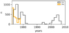 |
Fig. 1 Distribution of observations over the years. |
2 Observations, scanning, and data reduction
2.1 Brief description of the photographic plates used
Photographic observations of the main Saturnian satellites were performed at Pulkovo Observatory with the 26-inch refractor (hereafter P26; D = 0.65 m, F = 10.413 m) and the normal astrograph (hereafter PNA; D = 0.33 m, F = 3.463 m). Photographic plates of 13 × 18 cm and 16 × 16 cm in size were used for these astrographs, respectively. Hence, the effective field of view (FOV) is 30 × 30 arcmins for the P26 and 2 × 2 degrees for the PNA. The corresponding angular scales of the astronegatives are 19.8078 arcsec mm−1 and 59.56 arcsec mm−1.
These telescopes are located in Saint Petersburg (latitude 59°46′). Hence, the effective photographic observations of the Saturnian satellites with the PNA and P26 were limited to the declination (Dec) of − 10°. Therefore, Pulkovo astronomers organized observations of the Saturn system using telescopes in the Soviet Union’s more southern observatories. Unfortunately, only a limited number of these plates are available now. The results obtained with a small set of 14 of those plates are included in this paper. These plates were obtained with the Zeiss Double Astrograph (ZDA; D = 0.4 m, F = 3.024 m, FOV = 3.5 × 4.5 degrees, angular scale 68 arcsec mm−1) of the Abastumani Astrophysical Observatory in Georgia (Kiseleva et al. 2012) in 1984.
Regular observations of the Saturnian system were made from 1972 to 1984 when the declination of the planet was larger than −10 degrees. After a relatively long break, the observations resumed in the late 1990s and the last plate was taken in 2007. Figures 1 and 2 show the distribution of the observations in time and over the celestial sphere.
The total number of digitized photographic plates is 357. The number of exposures per astronegative varies from two to nine, with a shift of the plate cassette or the telescope between the exposures. Exposure times are distributed as shown in Table 1. It can be seen that 1-min and 3-min exposure times dominate in the P26 material, and the PNA sample manly contains images taken with 0.5-min, 1-min, and 2-min exposure times. The ZDA allowed us to take two plates at the same time. Exposure times of 1 min and 5 min were usually used for this telescope. Filters or coatings of the photographic plates for dimming the Saturn images were not applied.
Manual measurements of parts of these plates were performed with the Ascorecord measuring machine, and the equatorial and intersatellite coordinates were published with respect to the reference frames of various catalogs (from the third version of the Astronomische Gesellschaft Katalog (AGK3; Heckmann 1975) to the Positions and Proper Mothion Catalog (PPM; Roeser & Bastian 1988). The set of plates taken with the P26 between 1972 and 1974 was digitized with the Pulkovo Mobile Digitizing Device (MDD) digitizer (Izmailov et al. 2016), and the satellite positions were computed in the fourth USNO CCD Astrograph Catalog (UCAC4; Zacharias et al. 2013) frame (Kiseleva et al. 2015). This paper presents the results of the digitization and remeasurement of all plates with the Saturnian satellites (225 plates) from 1972 to 2007, the plates taken with the PNA from 1972 to 1977 (118), and 14 Georgian plates.
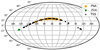 |
Fig. 2 Distribution of observations over the celestial sphere in equatorial coordinates. |
Number of exposures as a function of exposure time and instrument.
2.2 Digitization details
All measurements were performed with the Mobile Digitizing Device (MDD). This system allows us to scan a 12 cm × 12 cm area of each photographic plate. The image of the Saturn system fits this FOV for the P26, PNA, and ZDA astronegatives with a sufficient number of the second Gaia data release (Gaia DR2) stars. It is thereby possible to scan all the necessary parts of the photographic plate in one shot. We were able to set up the level of back illumination for the correct representation of the satellite images. Examples of scans are shown in Fig. 3. An opportunity to analyze all target images in one FOV of the camera is an advantage of the MDD. Relatively low resolution (MDD scale = 26 μm pix−1, P26 scale = 0.5 arcsec pix−1, PNA scale =1.6 arcsec pix−1) limits the astrometric quality. Moreover, the lens system has significant and unknown distortion for this FOV.
Thus, the success of the MDD scan calibration and the taking of systematic errors into account depended on the geometric stability of the device parts. The MDD digitizer was not equipped with a moving table or a rotator. The lens and astronegative frame were in rigid connection. These MDD features allowed us to solve the scan-to-scan stability problem.
The field distortion pattern of the MDD lens was investigated by comparing scans of the same plate taken with the MDD and the New Astrometric Reduction of Old Observations (NAROO1) digitizer located at the Paris Observatory (Robert et al. 2019). The NAROO digitizer scanning pipeline is based on the digitization of small overlapped sub-images (16.7 mm × 14 mm) with the scale ≈ 6.5 μm pix−1. The source images (stars and plate artifacts) were automatically detected with the Source Extracor (SExtractor; Bertin & Arnouts 1996) software. The cross-identification procedure was performed using the Delaunay triangulation algorithm (Delaunay 1934) and a search for the same triangles for each pair of the sub-images. Finally, an image merging procedure was followed. The transformation constants were calculated with the Nelder-Mead algorithm (Nelder & Mead 1965) to minimize the sum of squares of pixel-to-pixel signal differences of the overlapped parts of the images. Figure 4 shows the quality of the merging procedure. The constructed image is shown in Fig. 5. As a result, the template astronegative guarantees an accuracy of about ± 0.32 μm, which is sufficient for the MDD digitizer calibration.
Astronegative No. 43, with the image of Caldwell 14 filmed with the P26 (Fig. 5), was used as a “reference scan” for the MDD calibration. Scanning of this plate was performed twice in each digitizing session. Thus, the parameters of the transformation from each MDD distorted scan to the accurate reference NAROO scan were calculated for tens of MDD working sessions. Analysis of the residuals allowed us to construct the corresponding field distortion pattern (Fig. 6). As a result, the MDD-caused positional systematic errors were taken into account. The typical unit weight error of the MDD calibration is about 1 μm.
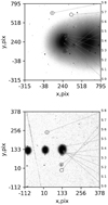 |
Fig. 3 Parts of astronegatives used in this paper. Upper panel: P26 plate No. 6035 taken at UTC = 1972-12-28T22:02:57. Bottom panel: extraction of ZDA astronegative No. 01655 filmed at UTC = 1984-06-15T18:37:38. The satellites designationsare S0 - Saturn, S1 - Mimas, S2 - Enceladus, S3 - Tethys, S4 - Dione, S5 - Rhea, S6 - Titan, S7 - Hyperion, and S8 - Iapetus. |
Number of Gaia reference stars per plate used for the astrometric reductions.
2.3 Stellar image centering and astrometric reduction
All of the Gaia DR2 reference stars and the satellite images were centered using the shapelet method (Refregier 2003; Khovrichev et al. 2018). The bright planet produced a huge scattered-light background gradient at the satellite image locations. A multi-scale median filter algorithm was applied to remove the background gradient. An example of the original image and the result of the gradient removal are displayed in Fig. 7.
Further astrometric calibration was performed with the linear model using the Gaia DR2 catalog as a reference. The number of reference stars depends on the exposure time, α, δ, and the telescope. The corresponding ranges of the reference star numbers are presented in Table 2. To avoid significant systematic errors, only stellar images located in the central part of the astronegatives were used for the ZDA. The positional residuals were analyzed to represent the averaged field distortion patterns for the P26 and PNA in various magnitude intervals. About 86 000 and 180 000 separate residuals for the Gaia stars were calculated for the P26 and PNA, respectively. In the case of the ZDA, a small number of astronegatives were available, not enough for an adequate investigation of the positional systematic errors. The vector fields for the P26 and PNA are displayed in Fig. 8. As can be seen, the distortion pattern depends on the magnitude. In some cases, the vector length achieves 0.1 arcsec. The area of the typical Saturnian satellite image locations is shown in Fig. 8 as a color map. Analysis of the Fig. 8 data shows that the positional systematic corrections are significant for the Saturnian satellite coordinate measurements. The field distortion patterns allow us to take x-dependant, y-dependent, and magnitude-dependent systematic errors into account through the interpolation of these vector fields. The color-dependent systematic errors are shown in Fig. 9. The Δα, Δδ residuals are shown for the central part of the plates where the satellite images are located. It can be seen that significant color-dependent correction with the value Δδ = −0.025 arcsec should be applied to the Titan positions that were measured with the PNA. As a result, the necessary corrections were applied and the final equatorial coordinates of the satellites were determined. We note that hereafter designations such as Δα, (O–C)α, σα, and εα are reduced values (multiplied by cosine δ).
An electronic table containing the equatorial coordinates of the main Saturnian satellites calculated in this study is available at the CDS.Table 3 is an extract.
 |
Fig. 4 Demonstration of the quality of the sub-image merging procedure. Images I1 and I2 are the same part of two different overlapped sub-images. I2-I1 is a result of subtraction. |
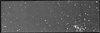 |
Fig. 5 Template scan constructed on the base of 30 sub-images taken with the NAROO digitizer. This is a part of plate No. 43 with the image of Caldwell 14 filmed with the P26 on October 16, 1957. |
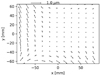 |
Fig. 6 Field distortion pattern for the NAROO-MDD template astronegative. |
 |
Fig. 7 Example of the Tethys (top peak), Dione (central peak), and Rhea (bottom peak) images, as well as the background brightness gradient structure. Left-hand panel: original image. The result of the subtraction of the gradient is presented in the right-hand panel. |
Extract from the CDS table that contains the equatorial coordinates of the main Saturnian satellites calculated in this study.
2.4 Statistical remarks and internal positional errors
Table 4 contains data regarding the number of observations for each satellite and the internal error values (ε). As described in Sect. 2.2, each plate was scanned four times and rotated by 90 degrees between scans. Measurement and astrometric reduction procedures give us four separate positions in equatorial coordinates for each exposure per satellite. The final α, δ of the satellite is the mean of the set of the four separate measurements. Naturally, we calculated standard deviations εα, εδ over the considered set. It appears that the mean values of the standard deviations are the same for both coordinates, and they are presented as ε values in Table 4.
The ε values independently characterize the quality of the digitization and image calibration. As mentioned in Sect. 2.2, the accuracy of the calibration of the MDD-scanned astronegatives is about 1 μm. For the P26, 1 μm corresponds to 20 mas. As can be seen from Table 4, accuracy is ≈1.5 times worse than expected, while the accuracy of the PNA and ZDA is at the predicted level (the PNA scale corresponds to 60 mas μm−1). As a result, the described approach of digitization and calibration allows us to reach a 1–1.5 μm accuracy level for the positional measurements of the satellite images on the photographic plates.
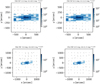 |
Fig. 8 Field distortion patterns for the P26 and PNA in different magnitude intervals. Each vector is an average of more than 100 separate residuals. Colored areas show the distribution of the satellite positions over the photographic plate. Color bars show the number of satellite images in a corresponding location. Top and bottom diagrams: results from the P26 and PNA, respectively, for bright (left) and faint (right) stars. |
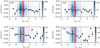 |
Fig. 9 Residuals for the Gaia stars as a function of color indices for the P26 and PNA satellite location areas. Red semi-transparent spans show the color indices of the main Saturnian satellites (the thin band at the GBP − GRP ≈ 1.9 mag represents Titan’s color). The (B–V) values for the Saturnian satellites were taken from Cruikshank (1978). They were converted to the Gaia color system according to Jordi et al. (2010). Color maps show the distribution of the differences over the color. Blue represents the number of differences in each bin, as indicated by the color bar. |
Number of observations and internal errors per coordinate (ε).
3 Comparison with the satellite ephemerides
A comparison of the resulted coordinates with the current version of the ephemerides and a search for possible trends that could potentially show ephemerides and/or observation imperfection are natural ways to understand the quality of the observational data. The natural satellites ephemerides facility MULTI-SAT (Emel’Yanov & Arlot 2008) was used to provide those comparisons. A combination of the planetary theory EPM-2017 (Pitjeva & Pitjev 2014) and satellite theory (Lainey et al. 2017) was adopted as the ephemeris source.
The results of the overall data comparison are presented in Tables 5 and 6. Table 5 shows that the mean residuals in both coordinates vary mostly within ± 25 mas from satellite to satellite for both telescopes, excluding the Hyperion (O–C)α for the PNA. This demonstrates a possible level of mutual systematic effects between the P26, the PNA, and the theories. The positional standard errors are in the 70–80 mas range, which is typical of similar studies (i.e., Robert et al. 2016). Table 6 shows preliminary estimates since only 14 plates were available.
3.1 Comparison between the 26-inch refractor and the normal astrograph results
As already mentioned, the P26 and PNA photographic plates were taken in a parallel mode on practically the same nights over five years. Hence, a mutual comparison of the (O–C) between the P26 and the PNA could reveal the telescope-dependent monotonic trends in the behavior of the residuals.
The images of the first four of the main Saturnian satellites were usually located within oversaturated areas caused by Saturn, due to the relatively short focal length of the PNA. Hence, the Rhea, Titan, and Iapetus positions form the main part of the PNA results.
Figure 10 provides examples of the (O–C) residual variations over time for Rhea and Iapetus. The (O–C) values for these satellites aremore suitable for comparison between the P26 and PNA data. It can be seen that the seasonal mean (O–C) values mostly lie within ±50 mas for both coordinates, and the results of both telescopes are usually overlapped within a 1-σ - 2-σ range, with the exception of several points. We believe that the P26 and PNA data contain a common part of the (O–C) trend over time.
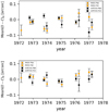 |
Fig. 10 Rhea and Iapetus mean RA, Dec residual variations vs. time for the P26 and the PNA. Each point is a result of averaging within the time intervals that correspond to the seasons of the observations. Error bars correspond to SEMs. |
3.2 Satellite minus Titan (O–C)
Traditionally, “satellite minus satellite” relative positions are calculated to eliminate the trends caused by planetary theory imperfections from the analysis. To avoid too many similar details, satellite minus Titan positional residuals for the P26 data are discussed below.
As expected, the positional accuracy for various satellites depends on an image’s signal-to-noise ratio. It should be looked at as a linear trend of the root mean square (RMS) residuals in the satellite minus Titan separations versus magnitude difference. The corresponding plot is presented in Fig. 11. As can be seen, such a trend does appear in the real data. It can be concluded that the accuracy of the P26 coordinates is higher than the accuracy of the PNA data because of the angular scale of the photographic plates.
Figure 12 displays the behavior of the seasonal mean values of satellite minus Titan (O–C) for both coordinates for the P26 data. The standard errors of the mean (SEMs) of those seasonal mean valuesare shown as an error bar. The SEM values are usually in the range of 20 to 50 mas. There are no significant systematic trends in this representation of (O–C) values. Almost all residuals are within the ± 50 mas limits (about ±300 km at Saturn). This supports the conclusion that the results are in agreement with the satellite motion theory at the level of positional accuracy for considered sets of observations. Small deviations of a group of points from zero that are seen for both coordinates have a very low level of significance and can be explained by both ephemeris and observation imperfections.
Residual magnitude-dependent systematic errors can be revealed in the analysis of the satellite minus Titan (O–C) as a function of the satellite minus Titan magnitude difference. The corresponding plots are shown in Fig. 13. It can be seen that all (O–C) values are close to zero except for Rhea (O–C)α and Tethys (O–C)δ. All (O–C)α values are positive. There is no evident (O–C) trend with a magnitude difference that can be explained by the presence of a significant residual magnitude equation. The variations may be caused by both residual observational systematic effects and the real systematic imperfections of the ephemerides.
Mean (O–C) values in equatorial coordinates and error budget for the P26 and PNA.
Mean (O–C) values in equatorial coordinates and error budget for the ZDA.
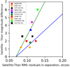 |
Fig. 11 RMS residuals in separation from Titan. The green line shows RMS increasing with magnitude for the P26 measurements. The blue line shows the same for the PNA. |
3.3 Comparison of the P26 data with the USNO photographic plate measurement results
A full series of photographic plates of the main Saturnian satellites taken with the USNO 26-inch refractor between 1974 and 1998 have been digitized with the Royal Observatory of Belgium (ROB) digitizer (De Cuyper et al. 2012); the remeasured and equatorial coordinates have been published (Robert et al. 2016). The USNO Saturnian satellite astrometric observations program was similar to the Pulkovo observations described above. Therefore, a comparison between the Pulkovo and USNO results should give us more information about the quality of both data sets.
Analysis of the Table 5 data and the results of Robert et al. (2016) show that the mean residuals differ slightly from each other. This can be explained by mutual systematic effects and possible biases between the UCAC4, which was a reference in Robert et al. (2016), and the Gaia DR2 system.
Hence, a mutual analysis of the relative satellite minus satellite positions could show the presence of common trends in residuals variations. This comparison requires a representative number of points in bins for both data sets. The Iapetus-Titan pair data satisfy this requirement. Figure 14 contains two plots with the (O–C) of the Iapetus minus Titan positions as a function of the sidereal planetocentric longitude difference. The size of the bin was adopted according to the condition of a representative data sample forming. It can be concluded that both the P26 and USNO residuals change with longitude in a very similar manner in the case of a sufficient number of points. Therefore, it is most probable that both data sets contain a common part that comes from ephemerides.
4 Saturnian satellite close approaches to the Gaia stars
There is a well-known way to improve the accuracy of the astrometric data of Solar System bodies: using observations of their close approaches to the stars of fundamental catalogs (Kovalevsky 2009) or other satellites (Pascu 1994; Morgado et al. 2016). Gaia DR2 is characterized by unprecedentedly high positional accuracy and a relatively dense distribution of stars over the celestial sphere, which makes this type of astrometry particularly effective (Bikulova 2019). Therefore, a search for this event was included in our scan processing procedure.
Information about 51 events is available at the CDS. An extraction of this data set is presented in Table 7. An event was considered a close approach if the angular distance (ρ) between the star and the satellite was less than 1 arcmin. The minimal value of ρ is 10.6 arcsec, and the mean is 40 arcsec. In most cases, several exposures were analyzed. As a result, the mean internal errors of the determination of the relative position (Δα, Δδ) were estimated. The overall mean RMS events are 70 mas in both coordinates. Residuals means and SEMs are − 14± 23 mas in right ascension (RA) and 50 ± 23 mas in declination (Dec).
Unfortunately, the event sample is too small to form a satisfactory conclusion. However, our results show the potential of this method in improving the astrometric accuracy of old observations.
 |
Fig. 12 Satellite minus Titan positional residuals as a function of time. Each point is a result of averaging over the corresponding seasons of observations. The ephemerides of the main Saturnian satellites used in the calculations are from Lainey et al. (2017). |
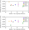 |
Fig. 13 Satellite minus Titan positional residuals as a function of magnitude difference. |
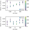 |
Fig. 14 P26 and USNO residuals variations for the Iapetus minus Titan positions vs. the sidereal planetocentric longitude difference. Each point is a result of averaging within the same longitude intervals. The colors indicate the number of separate residuals used to form mean values. Error bars show the SEMs. RA residuals are on top and Dec residuals are at the bottom. |
5 Conclusions
The results of the digitization and remeasurement of astrographic plates with the images of the main Saturnian satellites taken with the P26 and PNA at the Pulkovo observatory from 1972 to 2007 are presented in this paper. Data obtained by analyzing a small number of plates (14 astronegatives) filmed with the Abastumani ZDA are included.
The Pulkovo MDD digitizer was used to scan 357 photographic plates. The template astronegative was digitized by NAROO (Paris Observatory). A sub-image merging pipeline was developed and successively applied to calibrate the field distortion patterns of the MDD. A multi-scale median filter was implemented to remove scattered-light gradients in the images. The MDD accuracy of pixel x, y coordinate determination is 1–1.5 μm. As a result, equatorial coordinates of the main Saturnian satellites were calculated in the Gaia DR2 reference frame with an internal error of 30 mas for the P26 and 65 to 70 mas for the PNA and ZDA.
The electronic tables that contain the equatorial coordinates of the main Saturnian satellites and the parameters of the close approaches of the satellites to the Gaia DR2 stars are available online. A comparison of the satellite positions with the present-day ephemerides (EPM-2017+, Lainey et al. 2017) shows that the mean residuals are within ± 50 mas in the overwhelming number of cases. We can conclude that the observations are in good agreement with the theories on satellite motion. Coherent variations of the residuals revealed in the comparisons of our data with the USNO Saturnian photographic plate analysis results led to the estimation of systematic trends in the ephemerides that appeared in several decades of observations. The level of this systematic deviation is approximately 10 mas (about 60 km).
The results of the analysis of the close approaches of the Saturnian satellites to the Gaia stars are presented. They do not contradict the conclusions that are based on the main data (equatorial coordinates). Further analysis of these past events using old astrographic plates can be considered as a prospective method for future investigations.
Extract from the CDS table that contains the results of observations of Saturnian satellites’ close approaches to the Gaia stars.
Acknowledgements
The reported study was funded by RFBR according to the research projects No 19-02-00843 A and No 19-32-90175 (Sect. 4) and with partial support of the grant 075-15-2020-780 of the Government of the Russian Federation and the Ministry of Higher Education and Science. The NAROO program was supported by the DIM-ACAV of Ile-de-France region, PSL Research University, the Programme National GRAM and the Programme National de Planétologie (PNP) of CNRS/INSU with INP and IN2P3, co-funded by CNES. This work has made use of data from the European Space Agency (ESA) mission Gaia (https://www.cosmos.esa.int/gaia), processed by the Gaia Data Processing and Analysis Consortium (DPAC, https://www.cosmos.esa.int/web/gaia/dpac/consortium). Funding for the DPAC has been provided by national institutions, in particular the institutions participating in the Gaia Multilateral Agreement. Authors express their thanks to MULTI-SAT (http://nsdb.imcce.fr/multisat/) service developers. The authors are grateful to the referee for critical remarks, which led to improvements in the paper.
References
- Bertin, E., & Arnouts, S. 1996, A&AS, 117, 393 [NASA ADS] [CrossRef] [EDP Sciences] [Google Scholar]
- Bikulova, D. A. 2019, Contrib. Astron. Observ. Skalnate Pleso, 49, 459 [Google Scholar]
- Cruikshank, D. P. 1978, NASA Conf. Pub., 2068, 217 [Google Scholar]
- De Cuyper, J., de Decker, G., Laux, U., Winter, L., & Zacharias, N. 2012, ASP Conf. Ser., 461, 315 [Google Scholar]
- Delaunay, B. 1934, Bull. Acad. Sci. dURSS, 6, 793 [Google Scholar]
- Emel’Yanov, N. V., & Arlot, J. E. 2008, A&A, 487, 759 [NASA ADS] [CrossRef] [EDP Sciences] [Google Scholar]
- Gaia Collaboration (Brown, A. G. A., et al.) 2018, A&A, 616, A1 [NASA ADS] [CrossRef] [EDP Sciences] [Google Scholar]
- Heckmann, O. 1975, AGK 3. Star catalogue of positions and proper motions north of -2.5 deg. declination, ed. W. Dieckvoss (Hamburg-Bergedorf: Hamburger Sternwarte) [Google Scholar]
- Izmailov, I. S., Roshchina, E. A., Kiselev, A. A., et al. 2016, Astron. Lett., 42, 41 [CrossRef] [Google Scholar]
- Jordi, C., Gebran, M., Carrasco, J. M., et al. 2010, A&A, 523, A48 [NASA ADS] [CrossRef] [EDP Sciences] [Google Scholar]
- Khovrichev, M. Y., Apetyan, A. A., Roshchina, E. A., et al. 2018, Astron. Lett., 44, 103 [CrossRef] [Google Scholar]
- Kiseleva, T. P., Izmailov, I. S., Kalinichenko, O. A., & Vasilieva, T. A. 2010, Sol. Syst. Res., 44, 60 [CrossRef] [Google Scholar]
- Kiseleva, T. P., Chanturiya, S. M., Vasil’eva, T. A., & Kalinichenko, O. A. 2012, Sol. Syst. Res., 46, 436 [CrossRef] [Google Scholar]
- Kiseleva, T. P., Vasil’eva, T. A., Izmailov, I. S., & Roshchina, E. A. 2015, Sol. Syst. Res., 49, 72 [NASA ADS] [CrossRef] [Google Scholar]
- Kiseleva, T. P., Vasil’eva, T. A., Roshchina, E. A., & Izmailov, I. S. 2016, Sol. Syst. Res., 50, 402 [CrossRef] [Google Scholar]
- Kovalevsky, J. 2009, Celest. Mech. Dyn. Astron., 104, 403 [CrossRef] [Google Scholar]
- Lainey, V., Karatekin, Ö., Desmars, J., et al. 2012, ApJ, 752, 14 [Google Scholar]
- Lainey, V., Jacobson, R. A., Tajeddine, R., et al. 2017, Icarus, 281, 286 [NASA ADS] [CrossRef] [Google Scholar]
- Lainey, V., Casajus, L. G., Fuller, J., et al. 2020, Nat. Astron., 4, 1053 [CrossRef] [Google Scholar]
- Morgado, B., Assafin, M., Vieira-Martins, R., et al. 2016, MNRAS, 460, 4086 [NASA ADS] [CrossRef] [Google Scholar]
- Nelder, J. A., & Mead, R. 1965, Comput. J., 7, 308 [Google Scholar]
- Pascu, D. 1994, Galactic and Solar System Optical Astrometry, eds. L. V. Morrison, & G. F. Gilmore (Cambridge: Cambridge University Press), 304 [Google Scholar]
- Pascu, D., & Schmidt, R. E. 1990, AJ, 99, 1974 [NASA ADS] [CrossRef] [Google Scholar]
- Pitjeva, E. V., & Pitjev, N. P. 2014, Celest. Mech. Dyn. Astron., 119, 237 [Google Scholar]
- Refregier, A. 2003, MNRAS, 338, 35 [NASA ADS] [CrossRef] [Google Scholar]
- Robert, V., Pascu, D., Lainey, V., et al. 2016, A&A, 596, A37 [CrossRef] [EDP Sciences] [Google Scholar]
- Robert, V., Desmars, J., & Arlot, J. E. 2019, SF2A-2019: Proceedings of the Annual meeting of the French Society of Astronomy and Astrophysics [Google Scholar]
- Roeser, S., & Bastian, U. 1988, A&AS, 74, 449 [NASA ADS] [Google Scholar]
- Zacharias, N., Finch, C. T., Girard, T. M., et al. 2013, AJ, 145, 44 [NASA ADS] [CrossRef] [EDP Sciences] [Google Scholar]
NAROO webpage https://omekas.obspm.fr/s/naroo-project/page/home
All Tables
Extract from the CDS table that contains the equatorial coordinates of the main Saturnian satellites calculated in this study.
Mean (O–C) values in equatorial coordinates and error budget for the P26 and PNA.
Extract from the CDS table that contains the results of observations of Saturnian satellites’ close approaches to the Gaia stars.
All Figures
|
Fig. 1 Distribution of observations over the years. |
| In the text | |
|
Fig. 2 Distribution of observations over the celestial sphere in equatorial coordinates. |
| In the text | |
|
Fig. 3 Parts of astronegatives used in this paper. Upper panel: P26 plate No. 6035 taken at UTC = 1972-12-28T22:02:57. Bottom panel: extraction of ZDA astronegative No. 01655 filmed at UTC = 1984-06-15T18:37:38. The satellites designationsare S0 - Saturn, S1 - Mimas, S2 - Enceladus, S3 - Tethys, S4 - Dione, S5 - Rhea, S6 - Titan, S7 - Hyperion, and S8 - Iapetus. |
| In the text | |
|
Fig. 4 Demonstration of the quality of the sub-image merging procedure. Images I1 and I2 are the same part of two different overlapped sub-images. I2-I1 is a result of subtraction. |
| In the text | |
|
Fig. 5 Template scan constructed on the base of 30 sub-images taken with the NAROO digitizer. This is a part of plate No. 43 with the image of Caldwell 14 filmed with the P26 on October 16, 1957. |
| In the text | |
|
Fig. 6 Field distortion pattern for the NAROO-MDD template astronegative. |
| In the text | |
|
Fig. 7 Example of the Tethys (top peak), Dione (central peak), and Rhea (bottom peak) images, as well as the background brightness gradient structure. Left-hand panel: original image. The result of the subtraction of the gradient is presented in the right-hand panel. |
| In the text | |
|
Fig. 8 Field distortion patterns for the P26 and PNA in different magnitude intervals. Each vector is an average of more than 100 separate residuals. Colored areas show the distribution of the satellite positions over the photographic plate. Color bars show the number of satellite images in a corresponding location. Top and bottom diagrams: results from the P26 and PNA, respectively, for bright (left) and faint (right) stars. |
| In the text | |
|
Fig. 9 Residuals for the Gaia stars as a function of color indices for the P26 and PNA satellite location areas. Red semi-transparent spans show the color indices of the main Saturnian satellites (the thin band at the GBP − GRP ≈ 1.9 mag represents Titan’s color). The (B–V) values for the Saturnian satellites were taken from Cruikshank (1978). They were converted to the Gaia color system according to Jordi et al. (2010). Color maps show the distribution of the differences over the color. Blue represents the number of differences in each bin, as indicated by the color bar. |
| In the text | |
|
Fig. 10 Rhea and Iapetus mean RA, Dec residual variations vs. time for the P26 and the PNA. Each point is a result of averaging within the time intervals that correspond to the seasons of the observations. Error bars correspond to SEMs. |
| In the text | |
|
Fig. 11 RMS residuals in separation from Titan. The green line shows RMS increasing with magnitude for the P26 measurements. The blue line shows the same for the PNA. |
| In the text | |
|
Fig. 12 Satellite minus Titan positional residuals as a function of time. Each point is a result of averaging over the corresponding seasons of observations. The ephemerides of the main Saturnian satellites used in the calculations are from Lainey et al. (2017). |
| In the text | |
|
Fig. 13 Satellite minus Titan positional residuals as a function of magnitude difference. |
| In the text | |
|
Fig. 14 P26 and USNO residuals variations for the Iapetus minus Titan positions vs. the sidereal planetocentric longitude difference. Each point is a result of averaging within the same longitude intervals. The colors indicate the number of separate residuals used to form mean values. Error bars show the SEMs. RA residuals are on top and Dec residuals are at the bottom. |
| In the text | |
Current usage metrics show cumulative count of Article Views (full-text article views including HTML views, PDF and ePub downloads, according to the available data) and Abstracts Views on Vision4Press platform.
Data correspond to usage on the plateform after 2015. The current usage metrics is available 48-96 hours after online publication and is updated daily on week days.
Initial download of the metrics may take a while.