| Issue |
A&A
Volume 645, January 2021
|
|
|---|---|---|
| Article Number | A16 | |
| Number of page(s) | 12 | |
| Section | Planets and planetary systems | |
| DOI | https://doi.org/10.1051/0004-6361/202038934 | |
| Published online | 21 December 2020 | |
TOI-519 b: A short-period substellar object around an M dwarf validated using multicolour photometry and phase curve analysis
1
Instituto de Astrofísica de Canarias (IAC),
38200 La Laguna,
Tenerife,
Spain
e-mail: This email address is being protected from spambots. You need JavaScript enabled to view it.
2
Department Astrofísica, Universidad de La Laguna (ULL),
38206
La Laguna,
Tenerife, Spain
3
Centro de Astrobiologia (CSIC-INTA),
Carretera de Ajalvir km 4,
28850
Torrejon de Ardoz,
Madrid, Spain
4
Department of Earth and Planetary Science, The University of Tokyo,
Tokyo,
Japan
5
Komaba Institute for Science, The University of Tokyo,
3-8-1 Komaba,
Meguro,
Tokyo
153-8902, Japan
6
Japan Science and Technology Agency, PRESTO,
3-8-1 Komaba,
Meguro,
Tokyo
153-8902, Japan
7
Astrobiology Center,
2-21-1 Osawa,
Mitaka,
Tokyo
181-8588, Japan
8
National Astronomical Observatory of Japan,
2-21-1 Osawa,
Mitaka,
Tokyo
181-8588, Japan
9
Department of Physics and Astronomy, Vanderbilt University,
Nashville,
TN
37235, USA
10
Department of Astronomy, The University of Tokyo,
7-3-1 Hongo,
Bunkyo-ku,
Tokyo
113-0033, Japan
11
Center for Astrophysics, Harvard & Smithsonian,
60 Garden Street,
Cambridge,
MA
02138,
USA
12
Rheinisches Institut für Umweltforschung an der Universität zu Köln, Abteilung Planetenforschung,
Aachener Str. 209,
50931
Köln, Germany
13
Key Laboratory of Planetary Sciences, Purple Mountain Observatory, Chinese Academy of Sciences,
Nanjing
210023, PR China
14
European Space Agency (ESA), European Space Research and Technology Centre (ESTEC),
Keplerlaan 1,
2201 AZ
Noordwijk,
The Netherlands
15
Institute of Planetary research, German Aerospace Center,
Rutherfordstrasse 2,
12489
Berlin, Germany
16
Department of Astronomical Science, The Graduated University of Advanced Studies,
SOKENDAI, 2-21-1, Osawa,
Mitaka,
Tokyo
181-8588, Japan
17
Department of Astronomy and Tsinghua Centre for Astrophysics, Tsinghua University,
Beijing
100084,
PR China
18
George Mason University, 4400 University Drive,
Fairfax,
VA
22030,
USA
19
Department of Physics & Astronomy,
Swarthmore College,
Swarthmore
PA
19081, USA
20
University of Maryland,
Baltimore County, 1000 Hilltop Circle,
Baltimore,
MD
21250, USA
21
NASA Ames Research Center,
Moffett Field,
CA
94035, USA
22
SETI Institute,
189 Bernardo Avenue, Suite 100,
Mountain View,
CA
94043, USA
23
Noqsi Aerospace Ltd.,
15 Blanchard Avenue,
Billerica,
MA
01821, USA
24
Harvard-Smithsonian Center for Astrophysics,
60 Garden St.,
Cambridge,
MA
02138,
USA
25
Department of Physics and Kavli Institute for Astrophysics and Space Research, Massachusetts Institute of Technology,
Cambridge,
MA
02139,
USA
26
Space Telescope Science Institute,
3700 San Martin Drive,
Baltimore,
MD
21218, USA
27
Department of Aeronautics and Astronautics, Massachusetts Institute of Technology,
Cambridge,
MA
02139,
USA
28
Department of Earth, Atmospheric, and Planetary Sciences, Massachusetts Institute of Technology,
Cambridge,
MA
02139, USA
29
Department of Astrophysical Sciences, Princeton University,
Princeton,
NJ
08544, USA
Received:
15
July
2020
Accepted:
19
November
2020
Abstract
Context. We report the discovery of TOI-519 b (TIC 218795833), a transiting substellar object (R = 1.07 RJup) orbiting a faint M dwarf (V = 17.35) on a 1.26 d orbit. Brown dwarfs and massive planets orbiting M dwarfs on short-period orbits are rare, but more have already been discovered than expected from planet formation models. TOI-519 is a valuable addition to this group of unlikely systems, and it adds towards our understanding of the boundaries of planet formation.
Aims. We set out to determine the nature of the Transiting Exoplanet Survey Satellite (TESS) object of interest TOI-519 b.
Methods. Our analysis uses a SPOC-pipeline TESS light curve from Sector 7, multicolour transit photometry observed with MuSCAT2 and MuSCAT, and transit photometry observed with the LCOGT telescopes. We estimated the radius of the transiting object using multicolour transit modelling, and we set upper limits for its mass, effective temperature, and Bond albedo using a phase curve model that includes Doppler boosting, ellipsoidal variations, thermal emission, and reflected light components.
Results. TOI-519 b is a substellar object with a radius posterior median of 1.07 RJup and 5th and 95th percentiles of 0.66 and 1.20 RJup, respectively, where most of the uncertainty comes from the uncertainty in the stellar radius. The phase curve analysis sets an upper effective temperature limit of 1800 K, an upper Bond albedo limit of 0.49, and a companion mass upper limit of 14 MJup. The companion radius estimate combined with the Teff and mass limits suggests that the companion is more likely a planet than a brown dwarf, but a brown-dwarf scenario is a priori more likely given the lack of known massive planets in ≈ 1 day orbits around M dwarfs with Teff < 3800 K, and given the existence of some (but few) brown dwarfs.
Key words: stars: individual: TIC 218 795 833 / planets and satellites: general / methods: statistical / techniques: photometric
51 Pegasi b Fellow.
© ESO 2020
1 Introduction
Current planet formation models predict a very low probability for a low-mass star to harbour a brown dwarf or a massive planet on a short-period orbit (Mordasini et al. 2012), and M dwarf planet occurrence rate studies based on the Kepler data have corroborated this paucity (Dressing & Charbonneau 2015). However, contrary to expectations, a set of such objects have been discovered in recent years. Five brown dwarfs1 and four gas-giant planets2 are currently known to orbit M dwarf hosts cooler than 4000 K with orbital periods smaller than five days. The formation and subsequent evolution of these systems is an open question, as is their actual prevalence. A larger sample is required to find out whether the currently known systems are all rare objects, born from random formation accidents, or whether these systems belong to a family with a common formation path.
The Transiting Exoplanet Survey Satellite (TESS; Ricker et al. 2014) recently completed the second half of its two-year primary mission, and has discovered over two thousand transiting planet candidates (TESS objects of interest, or TOIs) to date. However, since various astrophysical phenomena can lead to a photometric signal mimicking an exoplanet transit (Cameron 2012), only a fraction of the candidates are legitimate planets (Moutou et al. 2009; Almenara et al. 2009; Santerne et al. 2012; Fressin et al. 2013), and the true nature of each individual candidate needs to be resolved by follow-up observations (Cabrera et al. 2017; Mullally et al. 2018). A mass estimate based on radial velocity (RV) measurements is the most reliable way to confirm a planet candidate, but RV observations are only practical for a subset of candidates (Parviainen et al. 2019).
We have recently reported the validation of TOI-263.01, which is a substellar companion orbiting an M dwarf on an extremely short-period orbit of 0.56 days (Parviainen et al. 2020). The validation was based on ground-based multicolour photometry following a multicolour transit modelling approach described in Parviainen et al. (2019). This approach models transit light curves observed in different passbands (filters) jointly, and yields posterior estimates for the usual quantities of interest (QOIs) in transiting planet light curve analysis, such as the orbital period, impact parameter, stellar density, andan estimate for the true companion radius ratio. The true radius ratio is a conservative radius ratio estimate3 that accounts for possible light contamination from unresolved objects inside the photometry aperture. The true radius ratio combined with a stellar radius estimate gives the absolute (conservative) radius of the companion, and if this is securely below the theoretical lower radius limit for a brown dwarf (~ 0.8 RJup, Burrows et al. 2011), the candidate can be considered to be a validated planet. If the true radius is ~ 1 RJup, the nature of the companion is ambiguous due to the mass-radius degeneracy for objects with masses in a gas giant planet and brown dwarf regime, and for radii larger than 1 RJup the probability that the object is a brown dwarf or a low-mass star increases rapidly.
We report the discovery of TOI-519 b, a transiting substellar object (0.66 RJup < R < 1.20 RJup, where the lower and upper limits correspond to the 5th and 95th percentiles, respectively) orbiting a faint M dwarf (TIC 218795833, see Table 1) on a 1.27 d orbit. The object was originally identified in the TESS Sector 7 photometry by the TESS Science Processing Operations Center (SPOC) pipeline (Jenkins et al. 2016), and was later followed up from the ground using multicolour transit photometry and low-resolution spectroscopy. The planet candidate passes all the SPOC data validation tests (Twicken et al. 2018), but the faint host star (V =17.35) makes radial velocity follow-up challenging. However, the large transit depth makes the system amenable to validation using multicolour transit photometry, although the uncertainties in estimating M dwarf radii complicate the situation by allowing solutions with R > 1.2 RJup. In this case, a radius estimate is not sufficient for validation, and we turned to phase-curve modelling to further constrain the companion’smass and effective temperature.
TOI-519 identifiers, coordinates, properties, and magnitudes.
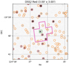 |
Fig. 1 TOI-519 and its surroundings observed by DSS with the TESS aperture used by the SPOC pipeline is shown in pink and TOI-519 is marked with a square. The nearest star, which is to the lower right of TOI-519, introduces a significant amount of flux contamination in the TOI-519 light curve. |
2 Observations
2.1 TESS photometry
TESS observed TOI-519 b during Sectors 7 and 8. Sector 7 was observed for 24.4 days covering 18 transits with a two-minute cadence. Sector 8 was observed for 24.6 days covering 13 transits (some of the transits occur during useless sections of the light curve), but the two-minute time cadence is not available, and the light curve must be created from the full frame image (FFI) data.
We chose to use the Sector 7 presearch data conditioning (PDC) light curve (Stumpe et al. 2014, 2012; Smith et al. 2012), produced by the SPOC pipeline, for the analysis. We added the crowding correction (“CROWDSAP”)4 back, which was removed by the pipeline, since the crowding correction can introduce a bias into our parameter estimation if the crowding is overestimated by the SPOC pipeline5. The TOI-519 light curve can be expected to contain a significant amount of flux contamination from a nearby star with a similar brightness (see Fig. 1), and our parameter estimation approach leads to an independent TESS contamination estimate based on the differences in transit depths between the TESS and ground-based transit observations.
The TESS photometry used in the transit analysis consists of 18, 3.6 h-long windows of SPOC data from Sector 7 centred around eachtransit based on the linear ephemeris, and each subset was normalised to its median out-of-transit (OOT) levelassuming a transit duration of 2.4 h. The photometry has an average point-to-point (ptp) scatter of 18.7 parts per thousand (ppt). We did not detrend the photometry, but modelled the baseline in the transit analysis.
The phase curve analysis uses all the SPOC Sector 7 data, except for the transits. We also created long-cadence light curves for Sectors 7 and 8 using the ELEANOR package (Feinstein et al. 2019), since while the short transit duration makes long-cadence less-than-optimal for transit modelling, having two sectors of data instead of one could still be beneficial for the phase curve modelling. However, we were not able to produce light curves with ELEANOR that would have matched the SPOC-produced light curve in quality. The long-cadence light curves show significantly higher systematics, which made them useless in the phase curve analysis.
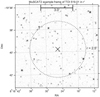 |
Fig. 2 MuSCAT2 field observed in r band. TOI-519 is marked with a cross, and the dotted circle marks the 2.5′ -radius region centred around TOI-519. |
2.2 MuSCAT2 photometry
We observed four full transits of TOI-519 b simultaneously in the g, r, i, and zs bands with the MuSCAT2 multicolour imager (Narita et al. 2019) installed at the 1.52 m Telescopio Carlos Sánchez (TCS) in the Teide Observatory, Spain, on the nights of 22 November 2019, 8 January 2020, 13 January 2020, and 29 February 2020. The exposure times were optimised on a per-night and per-CCD basis, but they were generally between 60 and 90 s. The observing conditions were excellent for all the nights (see Fig. 2 for an example frame).
The photometry was carried out using standard aperture photometry calibration and reduction steps with a dedicated MuSCAT2 photometry pipeline, as described in Parviainen et al. (2020). The pipeline calculates aperture photometry for the target and a set of comparison stars and aperture sizes, and it creates the final relative light curves via global optimisation of a model that aims to find the optimal comparison stars and aperture size, while simultaneously modelling the transit and baseline variations modelled as a linear combination of a set of covariates.
2.3 MuSCAT photometry
We also observed one full transit of TOI-519 b simultaneously in the g, r, and zs bands with the multicolour imager MuSCAT (Narita et al. 2015) mounted on the 1.88 m telescope at Okayama Astro-Complex on Mt. Chikurinji, Japan, on 30 November 2019. The observation was conducted for 3.4 h covering the transit, during which the sky condition was excellent. The telescope focus was slightly defocused so that the full width at half maximum (FWHM) of stellar point-spread function (PSF) was around 3′′. The exposure times were set at 60, 40, and 60 s in the g, r, and zs bands, respectively.
Image calibration (dark correction and flat fielding) and standard aperture photometry were performed using a custom pipeline (Fukui et al. 2011), with which the aperture size and comparison stars were optimised so that the point-to-point dispersion of the final light curve was minimised. The adopted aperture radius was 10 pixels (3.6′′) for all bands.
2.4 LCOGT photometry
Three full transits of TOI-519 b were observed using the Las Cumbres Observatory Global Telescope (LCOGT) 1 m network (Brown et al. 2013) in the g, i, and zs bands on the nights of 29 March 2019, 01 April 2019, and 16 April 2019, respectively. We used the TESS Transit Finder, which is a customised version of the Tapir software package (Jensen 2013), to schedule our transit observations. The g and zs transits were observed from the LCOGT node at Cerro Tololo Inter-American Observatory, Chile, and we used 60 and 150 s exposures, respectively. The i transit was observed from the LCOGT node at South Africa Astronomical Observatory, South Africa, and we used 150 s exposures. The 1 m telescopes are equipped with 4096 × 4096 pixel LCO SINISTRO cameras having an image scale of 0.′′389 pixel−1, resulting in a 26′ ×26′ field of view.
The images were calibrated by the standard LCOGT BANZAI pipeline (McCully et al. 2018) and the photometric data were extracted using the AstroImageJ (AIJ) software package (Collins et al. 2017). The g and zs images have PSFs with FWHM~1.′′8, and the i images were defocused resulting in FWHMs~3.′′2. Circular apertures with a radius of 11, 15, and 10 pixels were used to extract differential photometry in the g, i, and zs bands, respectively.
2.5 Spectroscopy
On 16 March 2020, we obtained the optical low-resolution spectrum of TOI-519 with the Alhambra Faint Object Spectrograph and Camera (ALFOSC) mounted at the 2.56 m Nordic Optical Telescope (NOT) on the Roque de los Muchachos Observatory. ALFOSC is equipped with a 2048×2064 CCD detector with a pixel scale of 0.2138′′ pixel−1. We used grism number 5 and a horizontal long slit with a width of 1.0′′, which yield a nominal spectral dispersion of 3.53 Å pixel−1 and a usable wavelength space coverage between 5000 and 9400 Å. Two spectra of 1800 s each were acquired at the parallactic angle and airmass of 1.51. ALFOSC observations of the white dwarf G191–B2B were acquired with the same instrumental setup as TOI-519, with an exposure time of 120 s, and at an airmass of 1.65. Raw images were reduced following standard procedures at optical wavelengths: bias subtraction, flat-fielding using dome flats, and optimal extraction using appropriate packages within the IRAF6 environment. Wavelength calibration was performed with a precision of 0.65 Å using He I and Ne I arc lines observed on the same night. The instrumental response was corrected using observations of the spectrophotometric standard star G191–B2B. Because the primary target and the standard star were observed close in time and at a similar airmass, we corrected for the absorption of telluric linesby dividing the target data by the spectrum of the standard, normalised to the continuum. The two individual spectra of TOI-519 were combined and the final spectrum, which has a spectral resolution of 16 Å (R ≈450 at 7100 Å), is depicted in Fig. 3.
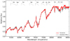 |
Fig. 3 Low-resolution spectrum observed with ALFOSC. The telluric-free optical spectrum of TOI-519 is shown in red (spectral resolution of 16 Å), and a solar-metallicity M4.0 spectral standard template from Kesseli et al. (2017) is plotted as the grey line (this spectrum has been degraded to the resolution of our target and it is also corrected for the telluric lines absorption). The most significant spectral features are labelled. The spectra are normalised to unity at around 7500 Å. |
3 Stellar characterisation
3.1 Low-resolution spectroscopy
We used the ALFOSC telluric-free spectrum to determine the spectral type of TOI-519 by measuring various spectroscopic indices, or colour ratios, that are suitable for M dwarfs. Some of these indices are nearly insensitive to the instrumental correction errors and their sensitivity to low and moderate extinction is also reduced, which makes them reliable indicators of spectral type. Other indices are useful as luminosity and metallicity discriminants. We obtained the flux ratios A, B/A, D/A, and TiO5 defined by Kirkpatrick et al. (1991) and Gizis (1997), all of which explore strong atomic lines and molecular bands present in M-type stars. Derived values and a short description of the features covered by the flux ratios are given in Table 2. All of these indices show very little dispersion in terms of spectral type and indicate that TOI-519 is an M3.0–M3.5 dwarf. This spectral type is fully consistent with the absolute magnitudes of TOI-519 in the optical through mid-infrared wavelengths (see next subsection).
However, spectral indices covering widely separated pseudo-continuum and feature regions yield later spectral types. The PC3 index defined by Martin et al. (1996), which measures the spectroscopic slope between two pseudo-continuum points of the optical data, delivers an M5 spectral type (Table 2). The best match to the ALFOSC spectrum among the data set of spectroscopic templates of Kesseli et al. (2017) is provided by the M4.0 spectral type as illustrated in Fig. 3. This discrepancy of about one spectral type may be explained by the presence of a moderate extinction or a higher metallicity. The former scenario, although feasible given the low Galactic latitude of our target (b ≈ +9 deg), is less likely because of the close distance to TOI-519. Also, GJHK and WISE colours are compatible with one single spectral type, which is a signpost of no or very little extinction towards TOI-519. Nevertheless, to explore the high metallicity scenario in detail, higher resolution spectra would be needed. To be conservative, we adopt a spectral type of M3.0–M4.5 for TOI-519.
From the ALFOSC spectrum, Hα is not seen in emission and we can impose a lower limit of 0.5 Å to the pseudo-equivalent width of any emission feature around 6563 Å. Potassium and sodium atomic lines, which are features that are rather sensitive to temperature and surface gravity, are seen in absorption with strengths similar to those of the M3.0–M4.5 standard stars. This suggests that TOI-519 has a high surface gravity, thus discarding the idea that our target is a very young or a giant star (and the atomic and molecular indices of Table 2 also reject the idea of our target being a giant or a subdwarf star).
From the spectral type – Teff relationship given in Houdebine et al. (2019), we derived 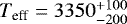 K for TOI-519, where the quoted errors account for spectral types in the interval of M3–M4.5. Houdebine et al. (2019) claim that their temperature calibration is valid for solar and near-solar metallicities; only strongly metal-depleted M dwarfs deviate from this calibration. TOI-519 does not show obvious absorption features due to hydrides (e.g. CaH) in the optical spectrum, which indicates that it is not a subdwarf (Kirkpatrick et al. 2014). Using various Teff -mass-stellar radii relationships available in the literature (e.g. Schweitzer et al. 2019; Houdebine et al. 2019; Cifuentes et al. 2020), we obtained that TOI-519 has a radius of
  R⊙ and a mass of
  M⊙. This mass determination is only slightly larger than that derived from Mann et al. (2019) relations, M⋆ = 0.36 ± 0.03 M⊙, and both values are consistent at the 1 σ level.
Spectroscopic indices and colour ratios.
3.2 Spectral energy distribution
As an independent determination of the stellar parameters, in particular the stellar radius, we performed an analysis of the broadband spectral energy distribution (SED) together with the Gaia DR2 parallax following the procedures described in Stassun & Torres (2016) and Stassun et al. (2017a,b). We used the grizy magnitudes from the Pan-Starrs database, the JHKS magnitudes from 2MASS, and the W1–W3 magnitudes from WISE. Together, the available photometry spans the full stellar SED over the wavelength range of 0.4–10 μm (see Fig. 4).
We performed a fit using NextGen stellar atmosphere models, adopting the effective temperature from the spectroscopically determined value. The extinction (AV) was set to zero due to the star being very close. The metallicity was left as a free parameter. The resulting fit, shown in Fig. 4, has a reduced χ2 of 2.5 and a best-fit metallicity of 0.0 ±0.5. Integrating the model SED gives the bolometric flux at Earth of Fbol = (3.20 ± 0.11) × 10−11 erg s−1 cm−2. Taking the Fbol and Teff together with the Gaia DR2 parallax, adjusted by + 0.08 mas in order to account for the systematic offset reported by Stassun & Torres (2018), gives the stellar radius of 0.342± 0.031 R⊙. Finally, we estimate a mass of 0.36 ± 0.03 M⊙ via Mann et al. (2019) empirical M-dwarf relations based on the absolute K-band magnitude. These values are in agreement with the values estimated from the low-resolution spectrum.
 |
Fig. 4 Spectral energy distribution of TOI 519. Red symbols represent the observed photometric measurements, where the horizontal bars represent the effective width of the passband. Blue symbols are the model fluxes from the best-fit NextGen atmosphere model (black). |
4 Light curve analysis
4.1 Overview
We modelled the TESS light curves simultaneously with the MuSCAT2, MuSCAT, and LCOGT light curves following the approach described in Parviainen et al. (2019, 2020) to characterise the system and obtain a robust “true radius ratio” estimate for the companion. Next, we carried out a phase curve analysis using the TESS light curve to constrain the companion’s effective temperature and mass. As a double check, we also carried out separate analyses using only the TESS or the ground-based data, but we do not detail those here. We have assumed zero eccentricity in all the analyses given the short circularisation time scales for a one-day period (Dawson & Johnson 2018).
The analyses were carried out with a custom Python code based on PYTRANSIT v27 (Parviainen 2015; Parviainen et al. 2019), which includes a physics-based contamination model based on the PHOENIX-calculated stellar spectrum library by Husser et al. (2013). The limb darkening computations were carried out with LDTK 8 (Parviainen & Aigrain 2015), and Markov chain Monte Carlo (MCMC) sampling was carried out with EMCEE (Foreman-Mackey et al. 2013; Goodman & Weare 2010). The code relies on the following PYTHON packages for scientific computing and astrophysics: SCIPY, NUMPY (van der Walt et al. 2011), ASTROPY (Astropy Collaboration 2013, 2018), PHOTUTILS (Bradley et al. 2019), ASTROMETRY.NET (Lang et al. 2010), IPYTHON (Perez & Granger 2007), PANDAS (Mckinney 2010), XARRAY (Hoyer & Hamman 2017), MATPLOTLIB (Hunter 2007), and SEABORN. The analyses are publicly available from GitHub9 as Jupyter notebooks.
4.2 Multicolour transit analysis
The final multicolour photometry dataset consists of the 18 transits in the TESS data from Sector 7; four transits observed simultaneously in four passbands (g, r, i, and zs) with MuSCAT2, one transit observed in three passbands (g, r, and zs) with MuSCAT, and two transits observed in two passbands (i and z) with the LCOGT telescopes. This sums up to five passbands (we consider z and zs to be the same), 25 transits, and 39 light curves.
The analysis followed standard steps for Bayesian parameter estimation (Parviainen 2018). First, we constructed a flux model that aims to reproduce the transits and the light curve systematics. Next, we defined a noise model to explain the stochastic variability in the observations not explained by the deterministic flux model. Combining the flux model, the noise model, and the observations gave us the likelihood. Finally, we defined the priors on the model parameters, after which we estimated the joint parameter posterior distribution using MCMC sampling.
The posterior estimation begins with a global optimisation run using differential evolution (Storn & Price 1997; Price et al. 2005) that results with a population of parameter vectors clumped close to the global posterior mode. This parameter vector population was then used as a starting population for the MCMC sampling with EMCEE, and the sampling was carried out until a suitable posterior sample was obtained (Parviainen 2018). The model parametrisation, priors, and the construction of the posterior function directly followed Parviainen et al. (2020).
4.3 Phase curve analysis
While multicolour transit analysis allowed us to securely estimate the companion’s radius ratio, modelling variations in the TESS light curve over its orbital phase gave us a tool to estimate the companion’s effective temperature, Bond albedo, and mass (Loeb & Gaudi 2003; Mislis et al. 2012; Shporer 2017; Shporer et al. 2019). Phase curve modelling is a well-established method for companion mass estimation, and it has been widely used to study planets and brown dwarfs found by the CoRoT and Kepler missions (i.e. CoRoT-3b Mazeh & Faigler 2010; TrES-2b Barclay et al. 2012; Kepler-13b Shporer et al. 2011 and Mislis & Hodgkin 2012; Kepler-91b Lillo-Box et al. 2014 and Barclay et al. 2015; and Kepler-41b Quintana et al. 2013, to name a few, and homogeneous phase-curve studies have been also reported by Esteves et al. 2013; Angerhausen et al. 2015; and Esteves et al. 2015).
The main four components contributing to the phase curve are Doppler boosting, ellipsoidal variations, reflection, and thermal emission, as illustrated in Fig. 5. The relative importance of the different effects depends on the orbital geometry, the host star, and the companion properties. For example, the effects of Doppler boosting (Loeb & Gaudi 2003) are expected to be significantly more important than ellipsoidal variations for TOI-519 b, as visible from Fig. 6 depicting the peak-to-peak expected amplitudes for TOI-519 b.
Phase curve analysis can be useful in distinguishing between low-mass stars and substellar objects orbiting low-mass stars on short-periodorbits, and it can also be used to distinguish between brown dwarfs and planets if the photometric precision is sufficiently high. In our case, the host star is faint by TESS standards, and we do not expect to detect significant phase variability if the companion is a planet or a low-mass brown dwarf. If the companion were a low-mass star, however, Doppler boosting should give rise to a clearly detectable signal. Here, our goal is to derive upper limits for the amplitudes of the different components, which can then be translated into upper limits for the effective temperature, companion mass, and Bond albedo.
We modelled the TESS out-of-transit light curve with a phase curve model combining reflection, thermal emission, Doppler boosting, and ellipsoidal variations. The TESS data were prepared the same way as for the main transit light curve analysis, but we excluded the transits from the light curve. We also simplified the model slightly and fixed the radius ratio, zero epoch, orbital period, orbital inclination, and semi-major axis to their median posterior values derived by the multicolour transit analysis (the uncertainties left in these quantities after the multicolour modelling have a very minor effect on the phase curve model), and we assumed a circular orbit.
The phase curve model is parameterised by the companion’s Bond albedo, AB, log companion mass, log Mp, host star mass, M⋆, and the effective temperatures of the host andthe companion, T⋆ and Tc, respectively.In its most abstract form, the model is a sum of a constant baseline level C (≈ 1) and the fourcomponents multiplied by their amplitudes
 (1)
(1)
where ϕ ∈ [0, 2π] is the orbital phase (ϕ = 0 for a transit), Ar Fr is the reflected light, At Ft is thermal emission, Ab Fb is the Doppler boosting, and AeFe is the ellipsoidal variation signal.
We approximated the planet as a Lambertian sphere10 (Russell 1916; Madhusudhan & Burrows 2012), for which the phase function is given as
 (2)
(2)
where k is the planet-star radius ratio, as is the scaled semi-major axis, α is the phase angle α = |ϕ − π|, and  is the eclipse function that is modelled as a transit over a uniform disk but with a depth scaled from 0 (full eclipse) to 1 (out of eclipse).
The thermal emission was simplified to give a constant contribution to the observed flux over the whole orbital phase except when the companion was occulted by the star. The contribution was a product of the planet-star area ratio and the planet-star flux ratio calculated by approximating the host star and the companion as black bodies,
 (3)
(3)
where T is the TESS passband transmission, P is Planck’s law, and λ is the wavelength.
The expected Doppler boosting was calculated following Loeb & Gaudi (2003)
 (4)
(4)
where c is the speed of light, G is the gravitation constant, p is the orbital period, and β is the photon-weighted passband-integrated beaming factor (Bloemen et al. 2010), described as
 (5)
(5)
where Fλ is the stellar flux at wavelength λ, and B = 5 + d logFλ∕d logλ is the beaming factor (Loeb & Gaudi 2003)11. The beaming factor was calculated based on a stellar spectrum modelled by Husser et al. (2013), rather than a black body approximation.
The ellipsoidal variation model follows that of Pfahl et al. (2008), assuming a circular orbit, and it is
 (6)
(6)
where u is the linear limb darkening coefficient, g is the gravity darkening coefficient, a is the semi-major axis, and R⋆ is the stellarradius.
We modelled the correlated noise in the light curve as a Gaussian process (GP) following an approximate Matérn 3/2 kernel using the celerite package (Foreman-Mackey et al. 2017). This is because the expected phase curve signal amplitudes are very small, and correlated noise could either lead to a false detection or mask an existing real signal and, especially, affect the posterior density tails. The flexibility from a GP model leads to a conservative analysis where we can be sure that we do not underestimate the component amplitudes allowed by the data, and that the derived upper limits are robust. The GP noise model is parametrised by log whitenoise, the log input scale, and the log output scale, all of which were kept free in the optimisation and posterior estimation.
We set a normal prior on the host star effective temperature of 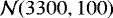 K and uniform priors on the log companion mass (from 0.3 to 300 MJup, also see the discussion about the posterior sensitivity on the prior and parametrisation in Sect. 6), effective temperature (from 500 to 3000 K), and Bond albedo (from 0 to 1). We set a normal prior on the log white noise standard deviation,
  , where ŝ is a white noise estimate calculated from the flux point-to-point scatter. The log GP input scale has a uniform prior
  , and the log output scale has a wide normal prior
  .
.
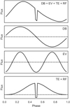 |
Fig. 5 Schematic showing Doppler boosting (DB), ellipsoidal variations (EV), thermal emission (TE), and reflection (RF) and all the phase curve components combined as a function of the orbital phase. |
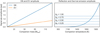 |
Fig. 6 Amplitudes of the four phase curve components for TOI-519 b as a function of the unknown companion mass, Bond albedo (Ab), and effective temperature. |
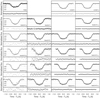 |
Fig. 7 Phase folded and binned TESS light curve, MuSCAT2 light curves, MuSCAT light curves, and LCOGT light curves together with the posterior median models and the residuals. The median baseline model was removed from the observed and modelled photometry for clarity. |
 |
Fig. 8 Marginal and joint posterior distributions for a set of parameters of interest from the joint light curve analysis. |
Relative and absolute estimates for the stellar and companion parameters derived from the multicolour transit analysis.
5 Results
We list the final parameter estimate in Table 3, and show the photometry used in the multicolour analysis with the transit model in Fig. 7; the posterior densities for the true radius ratio, the contaminant effective temperature, the impact parameter, and the stellar density in Fig. 8; and the final marginal posterior densities for the apparent and true radius ratio, and the apparent and true absolute radius in Fig. 9. The multicolour analysis gives a TESS contamination estimate of  , which allowed us to exclude significant flux contamination from sources of a different spectral type than the host in the ground-based photometry. This also allowed us to constrain the contamination from sources with the same spectral type as the host star to < 15% in the ground-based photometry. This leads to a median true radius ratio of 0.298 with a 5th percentile posterior lower limit of 0.290 and a 95th percentile posterior upper limit of 0.315.
The posterior densities for the companion mass, effective temperature, and Bond albedo from the phase curve analysis are shown in Fig. 10. The phase curve analysis leads to a Teff,C posterior that is uniform between 0 and 1750 K and then quickly slopes to zero. A tentative mode can be seen near 1700 K, but this is not statistically significant, and both the companion mass and Bond albedo have their modes at lower prior limit. The analysis allowed us to set an upper limit of 1800 K (corresponding to the 95th posterior percentile) for the companion Teff, an upper albedo limit of 0.49, and upper companion mass limit of 14 MJup. The companion mass posterior has a long tail, with a 99th percentile at ~ 22 MJup.
The companion mass posterior derived from the Doppler boosting and ellipsoidal variation signals can be sensitive to the prior set on the mass. We parameterised the companion mass using log mass on which we set a uniform prior, which translates to a non-uniform prior on the mass, since the companion mass is a “scale” parameter with an unknown magnitude (Gelman et al. 2013; Parviainen 2018). We tested the posterior sensitivity on the parameterisation, and while the body of the posterior changes, the95th posterior percentile is not affected significantly.
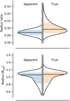 |
Fig. 9 Marginal posterior distributions for the apparent and true radius ratios (top), and the apparent and true absolute planet radii (bottom). The true radius ratio posterior has a long tail towards large values due to possible flux contamination. However, its effect on the absolute radius estimate is minor due to the large uncertainties in the stellar radius estimate. |
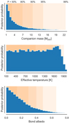 |
Fig. 10 Marginal posterior distributions for the companion mass, effective temperature, and Bond albedo. The orange-shaded areas shows a set of posterior percentile limits. |
6 Discussion and conclusions
The reliability of transiting planet candidate validation based on constraining the size of the transiting object crucially depends on the reliability of the stellar radius estimate. Large (~ 1 RJup) companions around low-mass stars are especially problematic due to the mass-radius degeneracy for objects in this radius regime and uncertainties in the low-mass star radii. For TOI-519 b, while the radius ratio is well-constrained, the companion’sabsolute radius depends on the stellar radius estimate based on M dwarf mass-radius relations and stellar classification based on low-resolution spectroscopy template matching. The companion radius posterior ranges from 0.66 RJup (certainly a planet) to 1.20 RJup (low-mass star or young brown dwarf). Only with the effective temperature and companion mass limits from the phase curve analysis canwe assess if the object is substellar.
The radius, effective temperature, and mass constraints from the multicolour and phase curve analyses validate TOI-519 b as a substellar object. That is, with R ~ 1 RJup, M < 14 MJup, and Tp < 1800 K, TOI-519 b is either a very low mass brown dwarf or a massive planet located in a very sparsely populated region in the period-radius space for substellar objects around M dwarfs. Here, the mass limit from the Doppler boosting creates a stronger constraint on the nature of the companion than the temperature limit, since the system is likely old enough that even a low-mass star could have cooled down below our detection threshold. Further, the upper mass limit favours the hypothesis that TOI-519 b is a planet rather than a brown dwarf, but a brown dwarf scenario is a priori strongly favoured. The currently known hot Jupiters around M dwarfs generally orbit hosts hotter than 3700 K with periods that are longer than 2 days, with the exception of Kepler-45b (see Fig. 11), and the (period, radius, host Teff) space that TOI-519 b falls in is dominated by brown dwarfs.
We caution that, in the case of TOI-519, the TESS crowding metric appears to be overestimated by the PDC pipeline. The CROWDSAP value that corresponds to the “ratio of target flux to the total flux in optimal aperture” is 0.51, corresponding to a contamination of 0.49, while our derived TESS contamination posterior median is 0.31. Our TESS contamination estimate can be considered secure since it is directly related to the differences in the apparent transit depths measured from the TESS and ground-based light curves. The ground-based transits are shallower than expected based on the crowding-corrected (PDC) TESS -observations, and this can only happen if the crowding is overestimated. Overestimated crowding leads to an overestimated radius ratio and, thus, an overestimated absolute radius. While this may be a rare occurrence, it is recommended to check for discrepancies between the TESS and ground-based photometry when carrying out a transit analysis and to include a free contamination factor for the TESS photometry if a joint transit analysis can be carried out with ground-based photometry.
Figure 11 shows TOI-519 b in the context of all currently known planets and brown dwarfs transiting cool host stars, and Fig. 12 extends these to include eclipsing M dwarf binaries. While the small number of objects does not allow us to make any statistically significant inferences, we can recognise some curious features whose significance will be uncovered in the future. First, all large (R > 0.5 RJup) objects, orbiting cool (Teff < 4000 K) dwarfs with periods shorter than 2 d are brown dwarfs. If TOI-519 b is confirmed to be a planet, it will be the only inhabitant of this parameter space. However, this feature is not very significant in the current context of low-number statistics, since all four of the known hot Jupiters orbiting M dwarfs have periods from 2 to 4 d (i.e. also relatively short). The lack of large objects around cool dwarfs in the period range of 4 to 200 d is more significant, but this can be largely due to observational biases; the figure includes only transiting objects with measured radii.
The lower panel of Fig. 11 shows a radius versus host stellar temperature. We note that giant planets and brown dwarfs seem to be found orbiting distinct spectral types. All large objects (R > 0.5 RJup) around the coolest dwarfs (Teff < 3400 K) are brown dwarfs, except for HATS-71 A b, and these transiting brown dwarfs seem to be clustered orbiting cool dwarfs with Teff~ 3100−3400 K. On the contrary, giant planets are found around spectral types with Teff> 3700 K. For the spectral types with Teff ~ 3400−3700 K, there is a desert of any companions with a R > 0.5 RJup. Whether this apparent clustering is of any significance needs to be verified by more hot Jupiter and brown dwarf discoveries around cool dwarfs.
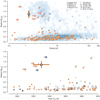 |
Fig. 11 TOI-519 b in the context of currently known transiting planet and brown dwarf systems. First (top), we show the radius as a function of the orbital period for transiting planets and brown dwarfs (BDs) with a focus on companions around cool (Teff <4000 K) host stars. Transiting planets around cool hosts are shown as orange-rimmed stars, transiting BDs around cool hosts as orange-rimmed circles, transiting BDs around hot hosts (Teff >4000 K) as dark-blue-rimmed circles, and transiting planets around hot hosts as blue-shaded areas. Next (bottom), we show the radius as a function of the effective temperature of the host star for transiting planets (stars) and brown dwarfs (circles). Objects with P < 1 d are coloured in dark blue, 1 < P < 5 d in orange, and P > 5 d in light grey. |
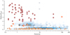 |
Fig. 12 TOI-519 b in the context of currently known transiting planet and brown dwarf systems and eclipsing M dwarf binaries marked as dark red circles. Otherwise as in Fig. 11. |
Acknowledgements
We thank the anonymous referee for their helpful and constructive comments. We acknowledge financial support from the Agencia Estatal de Investigación of the Ministerio de Ciencia, Innovación y Universidades and the European FEDER/ERF funds through projects ESP2013-48391-C4-2-R, AYA2016-79425-C3-2-P, AYA2015-69350-C3-2-P, and PID2019-109522GB-C53, and PGC2018-098153-B-C31. This work is partly financed by the Spanish Ministry of Economics and Competitiveness through project ESP2016-80435-C2-2-R. We acknowledge supports by JSPS KAKENHI Grant Numbers JP17H04574, JP18H01265, and JP18H05439, and JST PRESTO Grant Number JPMJPR1775. J.K. acknowledges support by Deutsche Forschungsgemeinschaft (DFG) grants PA525/18-1 and PA525/19-1 within the DFG Schwerpunkt SPP 1992, Exploring the Diversity of Extra-solar Planets. M.T. is supported by JSPS KAKENHI grant Nos. 18H05442, 15H02063, and 22000005. This work was partly supported by Grant-in-Aid for JSPS Fellows, Grant Number JP20J21872. This article is partly based on observations made with the MuSCAT2 instrument, developed by ABC, at Telescopio Carlos Sánchez operated on the island of Tenerife by the IAC in the Spanish Observatorio del Teide. We acknowledge the use of public TESS Alert data from pipelines at the TESS Science Office and at the TESS Science Processing Operations Center. This work makes use of observations from the LCOGT network. Resources supporting this work were provided by the NASA High-End Computing (HEC) Program through the NASA Advanced Supercomputing (NAS) Division at Ames Research Center for the production of the SPOC data products. This work makes use of observations from the LCOGT network.
References
- Almenara, J. M., Deeg, H. J., Aigrain, S., et al. 2009, A&A, 506, 337 [NASA ADS] [CrossRef] [EDP Sciences] [Google Scholar]
- Angerhausen, D., DeLarme, E., & Morse, J. A. 2015, PASP, 127, 1113 [NASA ADS] [CrossRef] [Google Scholar]
- Astropy Collaboration (Robitaille, T. P., et al.) 2013, A&A, 33, A1 [Google Scholar]
- Astropy Collaboration (Price-Whelan, A. M., et al.) 2018, AJ, 156, 123 [Google Scholar]
- Bakos, G. Á., Bayliss, D., Bento, J., et al. 2018, ArXiv e-prints [arXiv:1812.09406] [Google Scholar]
- Barclay, T., Huber, D., Rowe, J. F., et al. 2012, ApJ, 761, 53 [NASA ADS] [CrossRef] [Google Scholar]
- Barclay, T., Endl, M., Huber, D., et al. 2015, ApJ, 800, 46 [NASA ADS] [CrossRef] [Google Scholar]
- Bayliss, D., Gillen, E., Eigmüller, P., et al. 2018, MNRAS, 475, 4467 [NASA ADS] [CrossRef] [Google Scholar]
- Bloemen, S., Marsh, T. R., Østensen, R. H., et al. 2010, MNRAS, 410, 1787 [Google Scholar]
- Bradley, L., Sipocz, B., Robitaille, T., et al. 2019, https://doi.org/10.5281/ZENODO.2533376 [Google Scholar]
- Brown, T. M., Baliber, N., Bianco, F. B., et al. 2013, PASP, 125, 1031 [NASA ADS] [CrossRef] [Google Scholar]
- Burrows, A. S., Heng, K., & Nampaisarn, T. 2011, ApJ, 736, 47 [NASA ADS] [CrossRef] [Google Scholar]
- Cabrera, J., Barros, S. C. C., Armstrong, D., et al. 2017, A&A, 606, A75 [NASA ADS] [CrossRef] [EDP Sciences] [Google Scholar]
- Cameron, A. C. 2012, Nature, 492, 48 [NASA ADS] [CrossRef] [Google Scholar]
- Cifuentes, C., Caballero, J. A., Cortés-Contreras, M., et al. 2020, A&A, 642, A115 [NASA ADS] [CrossRef] [EDP Sciences] [Google Scholar]
- Collins, K. A., Kielkopf, J. F., Stassun, K. G., & Hessman, F. V. 2017, AJ, 153, 77 [NASA ADS] [CrossRef] [Google Scholar]
- Dawson, R. I., & Johnson, J. A. 2018, ARA&A, 56, 175 [NASA ADS] [CrossRef] [Google Scholar]
- Dressing, C. D., & Charbonneau, D. 2015, ApJ, 807, 45 [NASA ADS] [CrossRef] [Google Scholar]
- Esteves, L. J., De Mooij, E. J. W., & Jayawardhana, R. 2013, ApJ, 772, 51 [NASA ADS] [CrossRef] [Google Scholar]
- Esteves, L. J., Mooij, E. J. W. D., & Jayawardhana, R. 2015, ApJ, 804, 150 [NASA ADS] [CrossRef] [Google Scholar]
- Feinstein, A. D., Montet, B. T., Foreman-Mackey, D., et al. 2019, PASP, 131, 094502 [Google Scholar]
- Foreman-Mackey, D., Hogg, D. W., Lang, D., & Goodman, J. 2013, Publ. Astron. Soc. Pacific, 125, 306 [NASA ADS] [CrossRef] [Google Scholar]
- Foreman-Mackey, D., Agol, E., Ambikasaran, S., & Angus, R. 2017, AJ, 154, 220 [NASA ADS] [CrossRef] [Google Scholar]
- Fressin, F., Torres, G., Charbonneau, D., et al. 2013, ApJ, 766, 81 [NASA ADS] [CrossRef] [Google Scholar]
- Fukui, A., Narita, N., Tristram, P. J., et al. 2011, PASJ, 63, 287 [NASA ADS] [Google Scholar]
- Gelman, A., Carlin, J. B., Stern, H. S., et al. 2013, Bayesian Data Analysis, 3rd edn. (BOca Raton: CRC Press), 1 [Google Scholar]
- Gillen, E., Hillenbrand, L. A., David, T. J., et al. 2017, ApJ, 849, 11 [NASA ADS] [CrossRef] [Google Scholar]
- Gizis, J. E. 1997, AJ, 113, 806 [NASA ADS] [CrossRef] [Google Scholar]
- Goodman, J., & Weare, J. 2010, Commun. Appl. Math. Comput. Sci., 5, 65 [Google Scholar]
- Hartman, J. D., Bayliss, D., Brahm, R., et al. 2015, AJ, 149, 166 [NASA ADS] [CrossRef] [Google Scholar]
- Houdebine, É. R., Mullan, D. J., Doyle, J. G., et al. 2019, AJ, 158, 56 [CrossRef] [Google Scholar]
- Hoyer, S., & Hamman, J. J. 2017, J. Open Res. Softw., 5, 1 [CrossRef] [Google Scholar]
- Hunter, J. D. 2007, Comput. Sci. Eng., 9, 90 [NASA ADS] [CrossRef] [Google Scholar]
- Husser, T.-O., Wende-von Berg, S., Dreizler, S., et al. 2013, A&A, 553, A6 [NASA ADS] [CrossRef] [EDP Sciences] [Google Scholar]
- Irwin, J., Buchhave, L., Berta, Z. K., et al. 2010, ApJ, 718, 1353 [NASA ADS] [CrossRef] [Google Scholar]
- Irwin, J. M., Charbonneau, D., Esquerdo, G. A., et al. 2018, AJ, 156, 140 [NASA ADS] [CrossRef] [Google Scholar]
- Jackman, J. A. G., Wheatley, P. J., Bayliss, D., et al. 2019, MNRAS, 489, 5146 [NASA ADS] [CrossRef] [Google Scholar]
- Jenkins, J. M., Twicken, J. D., McCauliff, S., et al. 2016, in Proc. SPIE, 99133, 99133E [Google Scholar]
- Jensen, E. 2013, Astrophysics Source Code Library [record ascl:1306.007] [Google Scholar]
- Johnson, J. A., Gazak, J. Z., Apps, K., et al. 2012, AJ, 143, 111 [NASA ADS] [CrossRef] [Google Scholar]
- Kesseli, A. Y., West, A. A., Veyette, M., et al. 2017, ApJS, 230, 16 [NASA ADS] [CrossRef] [Google Scholar]
- Kirkpatrick, J. D., Henry, T. J., & McCarthy, Donald W., J. 1991, ApJS, 77, 417 [NASA ADS] [CrossRef] [Google Scholar]
- Kirkpatrick, J. D., Schneider, A., Fajardo-Acosta, S., et al. 2014, ApJ, 783, 2 [NASA ADS] [CrossRef] [Google Scholar]
- Lang, D., Hogg, D. W., Mierle, K., Blanton, M., & Roweis, S. 2010, AJ, 139, 1782 [Google Scholar]
- Lillo-Box, J., Barrado, D., Moya, A., et al. 2014, A&A, 562, A109 [NASA ADS] [CrossRef] [EDP Sciences] [Google Scholar]
- Loeb, A., & Gaudi, B. S. 2003, ApJ, 588, L117 [Google Scholar]
- Madhusudhan, N., & Burrows, A. S. 2012, ApJ, 747, 1 [NASA ADS] [CrossRef] [Google Scholar]
- Mann, A. W., Dupuy, T., Kraus, A. L., et al. 2019, ApJ, 871, 63 [NASA ADS] [CrossRef] [Google Scholar]
- Martin, E. L., Rebolo, R., & Zapatero-Osorio, M. R. 1996, ApJ, 469, 706 [NASA ADS] [CrossRef] [Google Scholar]
- Mazeh, T., & Faigler, S. 2010, A&A, 521, L59 [NASA ADS] [CrossRef] [EDP Sciences] [Google Scholar]
- McCully, C., Volgenau, N. H., Harbeck, D.-R., et al. 2018, SPIE Conf. Ser., 10707, 107070K [Google Scholar]
- Mckinney, W. 2010, Scipy, 1697900, 51 [Google Scholar]
- Mislis, D., & Hodgkin, S. 2012, MNRAS, 422, 1512 [NASA ADS] [CrossRef] [Google Scholar]
- Mislis, D., Heller, R., Schmitt, J. H. M. M., & Hodgkin, S. 2012, A&A, 538, A4 [NASA ADS] [CrossRef] [EDP Sciences] [Google Scholar]
- Mordasini, C., Alibert, Y., Benz, W., Klahr, H., & Henning, T. 2012, A&A, 541, A97 [NASA ADS] [CrossRef] [EDP Sciences] [Google Scholar]
- Moutou, C., Pont, F., Bouchy, F., et al. 2009, A&A, 506, 321 [NASA ADS] [CrossRef] [EDP Sciences] [Google Scholar]
- Mullally, F., Thompson, S. E., Coughlin, J. L., Burke, C. J., & Rowe, J. F. 2018, AJ, 155, 210 [NASA ADS] [CrossRef] [Google Scholar]
- Narita, N., Fukui, A., Kusakabe, N., et al. 2015, J. Astron. Telesc. Instrum. Syst., 1, 045001 [Google Scholar]
- Narita, N., Fukui, A., Kusakabe, N., et al. 2019, J. Astron. Telesc. Instrum., Syst., 5, 015001 [Google Scholar]
- Parviainen, H. 2015, MNRAS, 450, 3233 [Google Scholar]
- Parviainen, H. 2018, Handbook of Exoplanets (Cham: Springer International Publishing), 1 [Google Scholar]
- Parviainen, H., & Aigrain, S. 2015, MNRAS, 453, 3822 [Google Scholar]
- Parviainen, H., Tingley, B., Deeg, H. J., et al. 2019, A&A, 630, A89 [NASA ADS] [CrossRef] [EDP Sciences] [Google Scholar]
- Parviainen, H., Palle, E., Zapatero-Osorio, M. R., et al. 2020, A&A, 633, A28 [NASA ADS] [CrossRef] [EDP Sciences] [Google Scholar]
- Perez, F., & Granger, B. 2007, Comput. Sci. Eng., 9, 21 [Google Scholar]
- Pfahl, E., Arras, P., & Paxton, B. 2008, ApJ, 679, 783 [Google Scholar]
- Price, K., Storn, R., & Lampinen, J. 2005, Differential Evolution (Berlin: Springer) [Google Scholar]
- Quintana, E. V., Rowe, J. F., Barclay, T., et al. 2013, ApJ, 767, 137 [Google Scholar]
- Ricker, G. R., Winn, J. N., Vanderspek, R., et al. 2014, J. Astron. Telesc. Instrum. Syst., 1, 014003 [Google Scholar]
- Russell, H. N. 1916, ApJ, 43, 173 [Google Scholar]
- Santerne, A., Díaz, R. F., Moutou, C., et al. 2012, A&A, 545, A76 [NASA ADS] [CrossRef] [EDP Sciences] [Google Scholar]
- Schweitzer, A., Passegger, V. M., Cifuentes, C., et al. 2019, A&A, 625, A68 [NASA ADS] [CrossRef] [EDP Sciences] [Google Scholar]
- Shporer, A. 2017, PASP, 129, 72001 [Google Scholar]
- Shporer, A., Jenkins, J. M., Rowe, J. F., et al. 2011, AJ, 142, 195 [Google Scholar]
- Shporer, A., Wong, I., Huang, C. X., et al. 2019, AJ, 157, 178 [Google Scholar]
- Smith, J. C., Stumpe, M. C., Van Cleve, J. E., et al. 2012, PASP, 124, 1000 [Google Scholar]
- Stassun, K. G., & Torres, G. 2016, AJ, 152, 180 [Google Scholar]
- Stassun, K. G., & Torres, G. 2018, ApJ, 862, 61 [Google Scholar]
- Stassun, K. G., Collins, K. A., & Gaudi, B. S. 2017a, AJ, 153, 136 [Google Scholar]
- Stassun, K. G., Corsaro, E., Pepper, J. A., & Gaudi, B. S. 2017b, AJ, 155, 22 [Google Scholar]
- Storn, R., & Price, K. 1997, J. Glob. Optim., 11, 341 [Google Scholar]
- Stumpe, M. C., Smith, J. C., Van Cleve, J. E., et al. 2012, PASP, 124, 919 [Google Scholar]
- Stumpe, M. C., Smith, J. C., Catanzarite, J. H., et al. 2014, PASP, 126, 100 [Google Scholar]
- Twicken, J. D., Catanzarite, J. H., Clarke, B. D., et al. 2018, PASP, 130, 064502 [Google Scholar]
- van der Walt, S., Colbert, S. C., & Varoquaux, G. 2011, Comput. Sci. Eng., 13, 22 [Google Scholar]
TOI 263.01 by Parviainen et al. (2020), NGTS-7 A b by Jackman et al. (2019), LP 261-75b by Irwin et al. (2018), AD 3116 by Gillen et al. (2017), and NLTT 41135 b by Irwin et al. (2010).
Kepler-45b by Johnson et al. (2012), HATS-6b by Hartman et al. (2015), HATS-71b by Bakos et al. (2018), and NGTS-1b by Bayliss et al. (2018).
Here a “conservative radius ratio estimate” means that it should not underestimate the radius ratio, but rather give its reliable upper limit when assuming complete ignorance about the possible third light contamination.
The PDC crowding metric, C, corresponds to the ratio of the target flux to the total aperture flux, and the contamination defined in this paper, c, corresponds to the ratio of the contaminating flux to the total flux. The two are related as c = 1 − C.
As is the case here, see the Discussion for details.
Image Reduction and Analysis Facility (IRAF) is distributed by the National Optical Astronomy Observatories, which are operated by the Association of Universities for Research in Astronomy, Inc., under contract with the National Science Foundation.
Lambertian reflectance is admittedly a rather poor reflectance model for a gas giant or a brown dwarf, but sufficient for our purposes here.
Methods to calculate the photon-weighted passband-integrated beaming factor and the different phase curve components can be found from PYTRANSIT.
All Tables
Relative and absolute estimates for the stellar and companion parameters derived from the multicolour transit analysis.
All Figures
|
Fig. 1 TOI-519 and its surroundings observed by DSS with the TESS aperture used by the SPOC pipeline is shown in pink and TOI-519 is marked with a square. The nearest star, which is to the lower right of TOI-519, introduces a significant amount of flux contamination in the TOI-519 light curve. |
| In the text | |
|
Fig. 2 MuSCAT2 field observed in r band. TOI-519 is marked with a cross, and the dotted circle marks the 2.5′ -radius region centred around TOI-519. |
| In the text | |
|
Fig. 3 Low-resolution spectrum observed with ALFOSC. The telluric-free optical spectrum of TOI-519 is shown in red (spectral resolution of 16 Å), and a solar-metallicity M4.0 spectral standard template from Kesseli et al. (2017) is plotted as the grey line (this spectrum has been degraded to the resolution of our target and it is also corrected for the telluric lines absorption). The most significant spectral features are labelled. The spectra are normalised to unity at around 7500 Å. |
| In the text | |
|
Fig. 4 Spectral energy distribution of TOI 519. Red symbols represent the observed photometric measurements, where the horizontal bars represent the effective width of the passband. Blue symbols are the model fluxes from the best-fit NextGen atmosphere model (black). |
| In the text | |
|
Fig. 5 Schematic showing Doppler boosting (DB), ellipsoidal variations (EV), thermal emission (TE), and reflection (RF) and all the phase curve components combined as a function of the orbital phase. |
| In the text | |
|
Fig. 6 Amplitudes of the four phase curve components for TOI-519 b as a function of the unknown companion mass, Bond albedo (Ab), and effective temperature. |
| In the text | |
|
Fig. 7 Phase folded and binned TESS light curve, MuSCAT2 light curves, MuSCAT light curves, and LCOGT light curves together with the posterior median models and the residuals. The median baseline model was removed from the observed and modelled photometry for clarity. |
| In the text | |
|
Fig. 8 Marginal and joint posterior distributions for a set of parameters of interest from the joint light curve analysis. |
| In the text | |
|
Fig. 9 Marginal posterior distributions for the apparent and true radius ratios (top), and the apparent and true absolute planet radii (bottom). The true radius ratio posterior has a long tail towards large values due to possible flux contamination. However, its effect on the absolute radius estimate is minor due to the large uncertainties in the stellar radius estimate. |
| In the text | |
|
Fig. 10 Marginal posterior distributions for the companion mass, effective temperature, and Bond albedo. The orange-shaded areas shows a set of posterior percentile limits. |
| In the text | |
|
Fig. 11 TOI-519 b in the context of currently known transiting planet and brown dwarf systems. First (top), we show the radius as a function of the orbital period for transiting planets and brown dwarfs (BDs) with a focus on companions around cool (Teff <4000 K) host stars. Transiting planets around cool hosts are shown as orange-rimmed stars, transiting BDs around cool hosts as orange-rimmed circles, transiting BDs around hot hosts (Teff >4000 K) as dark-blue-rimmed circles, and transiting planets around hot hosts as blue-shaded areas. Next (bottom), we show the radius as a function of the effective temperature of the host star for transiting planets (stars) and brown dwarfs (circles). Objects with P < 1 d are coloured in dark blue, 1 < P < 5 d in orange, and P > 5 d in light grey. |
| In the text | |
|
Fig. 12 TOI-519 b in the context of currently known transiting planet and brown dwarf systems and eclipsing M dwarf binaries marked as dark red circles. Otherwise as in Fig. 11. |
| In the text | |
Current usage metrics show cumulative count of Article Views (full-text article views including HTML views, PDF and ePub downloads, according to the available data) and Abstracts Views on Vision4Press platform.
Data correspond to usage on the plateform after 2015. The current usage metrics is available 48-96 hours after online publication and is updated daily on week days.
Initial download of the metrics may take a while.