| Issue |
A&A
Volume 644, December 2020
|
|
|---|---|---|
| Article Number | A49 | |
| Number of page(s) | 9 | |
| Section | Stellar structure and evolution | |
| DOI | https://doi.org/10.1051/0004-6361/202039132 | |
| Published online | 30 November 2020 | |
Gaia18aen: First symbiotic star discovered by Gaia⋆
1
Astronomical Institute, Faculty of Mathematics and Physics, Charles University, V Holešovičkách 2, 180 00 Prague, Czech Republic
2
Institute of Physics, Faculty of Science, P. J. Šafárik University, Park Angelinum 9, 040 01 Košice, Slovakia
e-mail: This email address is being protected from spambots. You need JavaScript enabled to view it.
3
Nicolaus Copernicus Astronomical Center, Polish Academy of Sciences, Bartycka 18, 00–716 Warsaw, Poland
4
Astronomical Observatory, University of Warsaw, Al. Ujazdowskie 4, 00-478 Warszaw, Poland
5
Department of Physics and Astronomy, Texas Tech University, Box 41051, Science Building, Lubbock, TX 79409-1051, USA
6
Institute of Astronomy, University of Cambridge, Madingley Road, CB3 0HA Cambridge, UK
7
ICAMER Observatory of NASU, 27 Acad. Zabolotnoho Str., Kyiv 03143, Ukraine
8
Faculty of Physics, Taras Shevchenko National University of Kyiv, 4 Glushkova Ave., Kyiv 03022, Ukraine
9
Faulkes Telescope Project, School of Physics, and Astronomy, Cardiff University, The Parade, Cardiff CF24 3AA, UK
10
Astrophysics Research Institute, Liverpool John Moores University, 146 Brownlow Hill, Liverpool L3 5RF, UK
11
School of Physical Sciences, The Open University, Walton Hall, Milton Keynes MK7 6AA, UK
12
National Astronomical Research Institute of Thailand, 260, Moo 4, T. Donkaew, A. Mae Rim, Chiang Mai 50180, Thailand
13
Department of Physics and Astronomy, University of North Carolina at Chapel Hill, Chapel Hill, NC 27599, USA
14
Eastbury Community School, Hulse Avenue, Barking IG11 9UW, UK
Received:
10
August
2020
Accepted:
28
September
2020
Abstract
Context. Besides the astrometric mission of the Gaia satellite, its repeated and high-precision measurements also serve as an all-sky photometric transient survey. The sudden brightenings of the sources are published as Gaia Photometric Science Alerts and are made publicly available, allowing the community to photometrically and spectroscopically follow up on the object.
Aims. The goal of this paper is to analyze the nature and derive the basic parameters of Gaia18aen, a transient detected at the beginning of 2018. This object coincides with the position of the emission-line star WRAY 15-136. The brightening was classified as a “nova?” on the basis of a subsequent spectroscopic observation.
Methods. We analyzed two spectra of Gaia18aen and collected the available photometry of the object covering the brightenings in 2018 and also the preceding and following periods of quiescence. Based on this observational data, we derived the parameters of Gaia18aen and discussed the nature of the object.
Results. Gaia18aen is the first symbiotic star discovered by Gaia satellite. The system is an S-type symbiotic star and consists of an M giant of a slightly super-solar metallicity, where Teff ∼ 3500 K, a radius of ∼230 R⊙, and a high luminosity L ∼ 7400 L⊙. The hot component is a hot white dwarf. We tentatively determined the orbital period of the system ∼487 d. The main outburst of Gaia18aen in 2018 was accompanied by a decrease in the temperature of the hot component. The first phase of the outburst was characterized by the high luminosity L ∼ 27 000 L⊙, which remained constant for about three weeks after the optical maximum, later followed by the gradual decline of luminosity and increase of temperature. Several re-brightenings have been detected on the timescales of hundreds of days.
Key words: binaries: symbiotic / techniques: photometric / techniques: spectroscopic / stars: individual: Gaia18aen
Full Tables 3 and A.1 are only available at the CDS via anonymous ftp to cdsarc.u-strasbg.fr (130.79.128.5) or via http://cdsarc.u-strasbg.fr/viz-bin/cat/J/A+A/644/A49
© ESO 2020
1. Introduction
Symbiotic stars are among the widest interacting binaries. These stars consist of a cool giant (or a supergiant) of a spectral type M (in yellow symbiotics K, rarely G) as the donor and a compact star; most commonly a hot white dwarf (∼105 K) is the accretor (Mikołajewska 2007). These binaries are usually embedded in the circumbinary nebula created by the winds of both components. Thanks to their properties, symbiotic stars can serve as unique astrophysical laboratories to study accretion processes, winds, or jets (for more information see, e.g., reviews by Mikołajewska 2012; Munari 2019).
Most of the symbiotic stars in the previous century were discovered serendipitously as a result of their strong outbursts or during the spectroscopic surveys based on their peculiar spectral appearance. In recent years, several surveys focused on looking for new symbiotic stars in the Milky Way (e.g., Miszalski et al. 2013; Miszalski & Mikołajewska 2014; Rodríguez-Flores et al. 2014) and in external galaxies (e.g., Gonçalves et al. 2008, 2012, 2015; Kniazev et al. 2009; Mikołajewska et al. 2014, 2017; Iłkiewicz et al. 2018a).
In this paper, we report on the first discovery of the symbiotic star, Gaia18aen, by the Gaia satellite. Gaia18aen (AT 2018id, WRAY 15-136) was previously classified as an emission-line star by Wray (1966). Its outburst was detected by the Gaia satellite and announced by the Gaia Science Alert1 (GSA; Wyrzykowski & Hodgkin 2012; Hodgkin et al. 2013; Wyrzykowski et al. 2014) on January 17, 2018 (Delgado et al. 2018), when the star had the magnitude G = 11.33. In the alert, the transient was described as a bright emission-line star in Galactic plane which brightened by 1 magnitude. Previous measurements of the Gaia satellite over the period from October 31, 2014 to November 3, 2017 show the average magnitude of the star was 12.31 ± 0.10 with no significant changes. According to Gaia data, the star started to increase its brightness at the turn of November and December 2017. An observation obtained on December 3, 2017 revealed the star at a magnitude of 12.07 and the object continued to brighten in the following weeks. Kruszyńska et al. (2018) suggested a “nova?” classification for the object based on the spectrum obtained by VLT/X-shooter as a part of the program focused on spectroscopic classification of candidates for microlensing events. As it is discussed in this paper, the observed event was not a nova outburst, but a Z And-type outburst of a classical symbiotic star.
This paper is organized as followed: in Sect. 2 we discuss observational data, which were used for the classification of the object and analysis of its behavior and parameters, in Sect. 3 we describe spectra and light curves of the object, parameters of the symbiotic components, and discuss its variability and outburst activity.
2. Observations
2.1. Spectroscopy
We collected two spectroscopic observations of Gaia18aen. The first is a sequence of three low-resolution spectra obtained with the SPectrograph for the Rapid Acquisition of Transients (SPRAT) mounted on the Liverpool Telescope at La Palma (Steele et al. 2004) on January 20, 2018, under the program XOL17B02 (PI: Hodgkin). The exposure time of each spectrum is 30 s. The spectra have a wavelength range of 4000−8000 Å and a resolution R ∼ 350. The spectra were extracted, wavelength calibrated, and flux calibrated via the SPRAT pipeline (Piascik et al. 2014). In our analysis we used averaged spectrum.
Another spectroscopic observation was obtained by VLT/X-shooter (Vernet et al. 2011). Two exposures were obtained in the A-B nodding mode on March 22, 2018, under the program 0100.D-0021 (PI: Wyrzykowski). We used slits width 1.0″, 0.7″, 0.6″, which produced resolutions of 4300, 11 000, 7900, single exposures times were 91, 120, 10 s in the UV-Blue (UVB; 2989−5560 Å), Visible (VIS; 5337−10 200 Å), and near-infrared (NIR; 9940−24 790 Å) arms, respectively. We reduced the spectra with the dedicated EsoReflex pipeline (v. 3.3.4). The spectrum was corrected for telluric features using the MolecFit package (Kausch et al. 2015; Smette et al. 2015). We found this tool the most efficient to work with VLT/X-shooter data (see Ulmer-Moll et al. 2019). The standard procedure was applied, similar to those described for the VLT/X-shooter observations by Kausch et al. (2015), through fitting to the atmospheric absorption features from molecules of H2O and O2 in the visual range, and additionally CO2 and CH4 in the NIR.
VLT/X-shooter spectrum of Gaia18aen is shown in Fig. 1. A comparison of VLT/X-shooter spectrum down-sampled to the resolution of the Liverpool Telescope spectrum is shown in Fig. 2. The identification of the most prominent emission lines visible in the spectra of Gaia18aen is also shown in this figure. Detailed discussion of the spectral features is in Sect. 3.1.
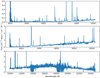 |
Fig. 1. VLT/X-shooter spectrum of Gaia18aen obtained on March 22, 2018. Upper panel: spectrum in the UBV arm, middle panel: in VIS arm, and bottom panel: spectrum obtained in the NIR arm. The spectrum was corrected for the telluric features (see the text). |
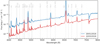 |
Fig. 2. Comparison of the two spectra of Gaia18aen obtained on January 20 and March 22, 2018 together with the identification of the major emission lines observed. |
2.2. Photometry
To study the photometric behavior of Gaia18aen before, during, and after its 2018 outburst, we collected all available photometric data from the databases of several surveys and from the literature to supplement the light curve in G filter obtained by Gaia. The data covering the active stage of Gaia18aen are collected by various telescopes participating in the follow-up network arranged under the time-domain work package of the European Commission’s Optical Infrared Coordination Network for Astronomy (OPTICON) grant2: Las Cumbres Observatory (LCO) 0.4 m, Panchromatic Robotic Optical Monitoring and Polarimetry Telescopes (PROMPT) 0.6 m, Terskol Observatory 0.6 m, and Physics Innovations Robotic Telescope Explorer (PIRATE) (Kolb et al. 2018). The data are available in B, V, R, i, g filters and were calibrated using the Cambridge Photometric Calibration Server (Zieliński et al. 2019, 2020). The calibration process is described in Sect. 2.1 of Wyrzykowski et al. (2020).
These data are supplemented by the data from the ASAS-SN survey (V and g filters; Shappee et al. 2014; Kochanek et al. 2017) and data in V and I from the OGLE IV survey (Udalski et al. 2015), covering mainly the pre-outburst phase (they are saturated during most of the outburst); ATLAS data in nonstandard orange and cyan filters (Tonry et al. 2018); and by the data from Bochum Survey of the Southern Galactic Disk (Haas et al. 2012; Hackstein et al. 2015) in r and i filters. All our photometric data are given in Table A.1.
Figure 7 shows the individual light curves of Gaia18aen obtained in various filters. We shifted the light curves to the same level for clarity; the values of these shifts are given in the figure legend. In Fig. 8, we show a section of the light curves showing the active stage of Gaia18aen in 2018.
3. Results and discussion
3.1. Spectral features and symbiotic classification
Spectroscopic observations of Gaia18aen revealed its symbiotic nature, satisfying the conditions of Belczyński et al. (2000), which are the presence of the absorption features of a late-type giant in the spectrum and of the emission lines of ions with an ionization potential (IP) of at least 35 eV. This classification is further confirmed by the presence of the O VI in the VLT/X-shooter spectrum (see Fig. 2).
Symbiotic classification of Gaia18aen is also supported by its position in diagnostic diagram using [O III] and Balmer lines fluxes and in the He I diagram (for more details, see, e.g., Iłkiewicz & Mikołajewska 2017; Iłkiewicz et al. 2018b). In both diagrams (see Figs. 1 and 4 in Iłkiewicz & Mikołajewska 2017), Gaia18aen is located in the region occupied solely by symbiotic stars ([O III] λ5006/Hβ = 0.04, [O III] λ4363/Hγ = 0.13; log(He Iλ6678/He Iλ5876) = −0.45, log(He Iλ7065/He Iλ5876) = −0.18).
In general, Gaia18aen shows an M-star continuum, superimposed with strong emission lines, mainly of H I and He I. A comparison of both our spectra shows significant changes in the intensity of the emission lines throughout the outbursts, for example, a significant decrease in the case of the high ionization lines of He II, [O III], [Fe VII], and O VI (see Sect. 3.4). For clarity of the comparison of both spectra (Fig. 2), we down-sampled the spectrum that was obtained by VLT/X-shooter to the resolution of the spectrum from the Liverpool Telescope (R ≈ 350). We also applied an absolute flux scale to the Liverpool Telescope spectrum using the average V = 12.8 mag such that convolution of the spectrum with the Johnson V filter agrees with the V mag. Table 2 gives the emission-line fluxes that were measured by fitting Gaussian profiles to the calibrated spectra.
3.2. Distance and reddening
Gaia DR2 gives for Gaia18aen a parallax 0.097 ± 0.054 mas yr−1 with goodness-of-fit statistic parameter gofAL ≈ 37, which indicates a very poor fit to the data. Bailer-Jones et al. (2018) inferred the distance to the sources from Gaia DR2 using the Bayesian approach, which is also suitable also for the objects with poor precision of the parallax and even for negative parallaxes. These authors obtained for Gaia18aen the distance 5.8 kpc placed in the asymmetric confidence interval from 4.6 kpc to 7.6 kpc.
The Na I D1, D2 interstellar line profiles reveal two distinct components that allowed us to assume a Doppler splitting caused by at least two diffuse ISM clouds, which may be present along the line of sight (see Siebenmorgen et al. 2020). In particular, radial velocities with respect to the local standard of rest (LSR), VLSR, derived from both Na I D1, D2 lines indicate a range of mean cloud velocities of ∼14 to 62 km s−1 (Fig. 3). If the velocity is due to Galactic rotation it can be used to derive a lower limit to distance. In particular, the component with the maximum velocity, VLSR = 62 km s−1, indicates d > ∼6 kpc. The radial velocity of the red giant component transformed to LSR, Vg, LSR ∼ 81 km s−1, would indicate a distance of ∼8 kpc. However, this estimate should be considered as an upper limit because the radial velocity of the giant can be affected by unknown orbital motion or pulsation.
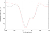 |
Fig. 3. Line profiles of the Na I D1 (black) and Na I D2 (red). |
As Gaia18aen is located in the Galactic disk (b = 0.314, Table 1), it is expected to be highly reddened. We estimate total Galactic extinction in its direction, E(B − V) = 1.17 using the maps of the Galactic extinction by Schlegel et al. (1998), and E(B − V) = 1.03 from those by Schlafly & Finkbeiner (2011), however, there are important caveats about unreliable extinction estimates for this position.
Basic properties of Gaia18aen.
Emission-line fluxes in 10−13 erg s−1 cm−2.
An independent reddening estimate can be derived from the emission-line ratios (Table 3). The H I Balmer lines are reliable reddening indicators only for negligible self-absorption in the lower series members (case B recombination; e.g., Cox & Mathews 1969; Netzer 1975). However, this is usually not the case for symbiotic stars (e.g., Mikołajewska et al. 1997), for which the reddening-free Hα/Hβ ratio is ∼5−10 (e.g., Mikołajewska & Kenyon 1992; Mikołajewska et al. 1995, 1997; Proga et al. 1994). The values of Hα:Hβ:Hγ:Hδ ratios measured in the spectrum of Gaia18aen, in fact, are inconsistent with case B recombination for any reddening. Fortunately, we can use He II lines, which are less prone to optical depth effects. The most useful for the reddening estimate He II Pickering line ratios (10124:5411:4542) and Pickering 10124 to Paschen 4686 ratio are consistent with case B and E(B − V) = 1.16 ± 0.01. A similar value, E(B − V) = 1.14, is indicated by the NIR H I Brγ:Paδ ratio, whereas a slightly higher E(B − V) = 1.25 provides a better match of the synthetic cool giant spectra to the observed NIR spectrum (see Sect. 3.3). We adopted d = 6 kpc and E(B − V) = 1.2 for the rest of this paper.
Positions, radial velocities, and fluxes of identified emission lines in the VLT/X-shooter spectrum of Gaia18aen obtained on March 22, 2018.
3.3. Cool component
The VLT/X-shooter spectrum of Gaia18aen was used to derive atmospheric parameters and the information about the chemical composition of the atmosphere of the cool component. In order to put constraints on the physical parameters of the atmosphere of the red giant, mainly its temperature and metallicity, we used the BT-NextGen grid of the theoretical spectra (Allard et al. 2011); these spectra are calculated using the solar abundances of Asplund et al. (2009), which are available from Theoretical spectra webserver at the SVO Theoretical Model Services3. Next, we used the 1D hydrostatic MARCS model atmospheres by Gustafsson et al. (2008) to perform a more detailed analysis of the chemical composition.
We searched among several hundreds of BT-NextGen models in the following range of parameters: Teff = 2900−4800 K, log g = −0.5 − 1.5, [M/H] = −2.5 to +0.5, and [α/H] = 0.0 to +0.4. All synthetic spectra were convolved with the Gaussian profile with the full width at half maximum corresponding to the velocity V = 149 km s−1 to achieve the final resolution R ∼ 2000. The VLT/X-shooter spectrum of Gaia18aen was heliocentric velocity corrected by −14.554 km s−1 and for the red giant velocity, Vg, hel = 99 km s−1, derived from the absorption lines in the NIR spectrum. This spectrum was then convolved with Gaussian profiles of v sin i = 145 km s−1 and v sin i = 147.5 km s−1 in the VIS and NIR ranges, respectively, to reduce its resolution to those adopted for the model spectra. The observed spectrum was de-reddened by EB − V = 1.25 using the Cardelli et al. (1989) reddening law and adopting total-to-selective absorption ratio R = 3.1 with the use of the VOSpec4 Virtual Observatory tool. The adopted initial value EB − V = 1.20 was replaced with EB − V = 1.25 to achieve better compliance in the J-band region.
Each spectrum was normalized with the flux value measured in a narrow (50 Å) range of the K-band region centered at 22 155 Å. The residuals were calculated for each pair of spectra (theoretical model and the observed spectrum) to obtain the χ2 value that characterizes the fit quality. Only selected ranges in the NIR of the H- and K-band regions were finally used in the residual calculations to exclude the areas disturbed by some artifacts. A shorter wavelength region was not taken into account because in the case of symbiotic systems the visual range is strongly dominated by the contribution from the hot component and the nebula, and there are numerous, strong emission lines present even in the J band (see Table 3).
The fit quality in the parameter space is illustrated in Fig. 4. We obtain the strongest dependence on temperature. The best solutions are obtained for Teff ∼ 3500 K. In the case of the remaining parameters, there is significant degeneration and the minimum is not clearly defined, however, in the case of metallicity the near solar values seem to be preferred. Taking into account the values of the scale factor (generally in the range Sf = 6.4 − 7.9 × 10⁻¹⁹ in the case of the best-matching models), we can limit the value of surface gravity log g ≈ 0.0 because the higher value could result in a mass of the giant that is too high. Figure 5 shows the comparison of the VLT/X-shooter spectrum with the synthetic model corresponding to the atmospheric parameters Teff = 3500 K, log g = 0.0, [M/H] = 0.0, and [α/H] = 0.0 close to those finally preferred from the spectral synthesis.
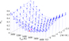 |
Fig. 4. Surface of χ2 in function of Teff and [M/H] parameters. Two selected cases are distinguished with red (the best match) and magenta (with atmospheric parameters close to those obtained via spectral synthesis fit; see Figs. 5 and 6). |
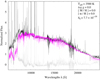 |
Fig. 5. Comparison of the VLT/X-shooter spectrum and the synthetic model. The VLT/X-shooter spectrum (black line) de-reddened by EB − V = 1.25 is compared with the synthetic model (magenta) corresponding to the following atmospheric parameters: Teff = 3500 K, log g = 0.0, [M/H] = 0.0, and [α/H] = 0.0. The residuals – observations minus calculations – are shown at the bottom with gray line. The spectra were normalized to the flux level at the narrow range (50 Å) centered at 22 155 Å. The scale factor is Sf = Fobs/Fmodel = 7.7 × 10⁻¹⁹. |
The elemental abundances of the particular elements were measured through the fit of the synthetic spectrum to the observed spectrum in the K-band region. The observed spectrum was normalized to the continuum level beforehand. We tested a number of the atmosphere models (MARCS; Gustafsson et al. 2008) with temperature and surface gravity set to constant values as follows: Teff = 3500 K, log g = 0.0. Various metallicities expressed in [Fe/H] were tested in the range −0.5 to +0.5 dex, including a sample of alpha-enhanced cases ([α/Fe] = +0.4 dex). The micro- (ξt) and macro- (ζt) turbulence velocities, were set to 2 km s−1 and 3 km s−1, respectively, which are the values typical for cool, Galactic red giants. The excitation potentials and gf values for transitions in the case of atomic lines were taken from the Vienna Atomic Line Database (Kupka et al. 1999). For the molecular data, we used line lists by Goorvitch (1994) for CO, R. L. Kurucz5 for OH, and Sneden et al. (2014) for CN. The spectrum synthesis was run using the WIDMO code (Schmidt et al. 2006) with the method as described by Gałan et al. (2017, and references therein). The best match was obtained for the model with slightly super-solar metallicity [Fe/H] = +0.25 dex and [α/Fe] = 0.0 dex with differences of abundances in relation to the model not larger than 0.11 dex in the case of elements that are best represented with atomic lines in the spectrum (i.e., Fe, Ti, Ca, and Na). The obtained abundances are listed in Table 4 and the synthetic fit to the observed spectrum is shown in Fig. 6.
Final values of abundances obtained from K-band region together with the formal fitting errors and 12C/13C isotopic ratio.
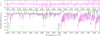 |
Fig. 6. VLT/X-shooter spectrum of Gaia18aen (black line) and synthetic spectrum (magenta line) calculated using the final abundances (Table 4). |
The relative [Ti/Fe] = −0.04 abundance compared to metallicity ([Fe/H] = 0.34) is consistent with the membership in Galactic disk (see Gałan et al. 2017, Fig. 7), whereas the [Ti/Fe] ratio in relation to [Ti/H] suggests that Gaia18aen belongs to the disk population < 7 Gyr in age (see Bensby et al. 2014). Practically all derived abundances in relation to iron ([Na/Fe], [Ca/Fe], [Ti/Fe], [Y/Fe]) are consistent with those expected for the disk population (Bensby et al. 2014). The only exceptions are [Mg/Fe] and [Si/Fe], which seems to indicate a large overabundance of these two elements. However, these abundances are less reliable because they are based on a few weak lines in the case of Si I or a single relatively strong feature, which is split into the number of lines in the case of Mg I. Our best solution for the model with [α/Fe] = 0.0 dex resulted in suspiciously low oxygen abundance ([O/H] = −0.66 ± 0.34); this is difficult to explain by the models of evolution in the symbiotic systems. The second best-fit model obtained for the same atmospheric parameters and enhanced [α/Fe] = 0.4 dex gives much more reliable value [O/H] = +0.06 ± 0.33 (Table 4). However, the abundances of oxygen and nitrogen as well as some other elements derived from atomic lines (e.g., Si, V, and Co) can be burdened with large errors that can account for some peculiarities of the obtained composition.
Skowron et al. (2019) mapped the shape of the Milky Way disk based on the distances to nearly 2500 classical Cepheids. In their coordinate system (R, ϕ, where R is the distance of the object from Galactic center and ϕ is the Galactocentric azimuth measured counterclockwise from l = 0°), Gaia18aen would be placed at R ∼ 11.5 kpc and ϕ ∼ 28°. At this location, the disk is bent south, however, the displacement of Gaia18aen away from the central disk surface is only ∼0.2 kpc north, that is, in agreement with its disk membership.
The NIR spectrum as well as 2MASS and WISE colors are all consistent with a non-dusty S-type symbiotic system. The scaling factor resulting from our best model fit combined with the distance to Gaia18aen implies a red giant radius of ∼230 R⊙ and luminosity of ∼7400 L⊙, which places Gaia18aen among the brightest symbiotic giants (e.g., Mikołajewska 2012).
The giants in S-type symbiotic systems often exhibit pulsations and, moreover, S-type systems have orbital periods on such timescales (∼300−600 d; Gromadzki et al. 2013), which should be detectable using the available data. We therefore used out-of-outburst data (OGLE I and GaiaG, with data from the period JD ∼ 2 458 000−2 458 500 excluded and ATLAS o and c, Bochum r, and (i) to search for any periodical changes. There are several clear minima in these quiescent light curves around JD ∼ 2 455 910, 2 456 355, 2 457 345 and 2 458 820, respectively. The periodicity that fits this data is written as
 (1)
(1)
ASAS-SN light curves were not used in this analysis because their coverage is insufficient (especially in g filter) or their scatter is larger than the amplitude in the best dataset (combined ATLAS o and GaiaG). The phased light curve in g, however, seems to show the same modulation, whereas it is less obvious in V. The phased light curve in selected filters is shown in Fig. 9.
We tentatively attributed the 487 d modulation to the orbital period of the system. Assuming the total mass of the system is ∼2−3 M⊙ (i.e., similar to other symbiotic stars; see, e.g., Mikołajewska 2003), we estimate the binary separation to be about 1.5−1.7 AU. The red giant with a radius of ∼230 R⊙ could then fill its Roche lobe. While there is some indication of a secondary minimum due to ellipsoidal variability in the phased light curve (Fig. 9), to fully confirm this finding and refine the period, a well-sampled, long-term light curve of Gaia18aen and measurements of radial velocities of the giant would be needed.
The large scatter in quiescent light curves may be due to additional short-term variations with timescales of 50−200 d caused by stellar pulsations of the red giant component of the binary system. This component can be either a semi-regular variable or a so-called OSARG (OGLE small amplitude red giant). Thus, the red giant in Gaia18aen would be very similar to red giants in S-type symbiotic systems from this point of view as well (see, e.g., Gromadzki et al. 2013, for more details about light curves of S-type symbiotics).
3.4. Hot component and outburst activity
The most prominent features in the light curves of Gaia18aen (Fig. 7) are the outbursts observed in 2018. In Fig. 8, the part of the light curve showing the active stage is depicted. For clarity, the light curves in various filters were shifted to the same level to study the structure of the active stage. Individual brightenings are labeled by the numbers 0−5.
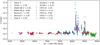 |
Fig. 7. Light curves of Gaia18aen. Individual light curves in various filters were shifted to the level in the OGLE V filter for clarity; values of shifts are shown in the figure legend. Different colors denote different filters. |
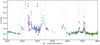 |
Fig. 8. Outbursts of Gaia18aen. The colors are the same as in Fig. 7. The vertical dotted lines indicate the individual brightenings (denoted by numbers 0−5). The arrows show the times when the two spectra were obtained. |
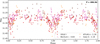 |
Fig. 9. Light curves in selected filters phased with the period of P = 486.9 d. Individual datasets were shifted to the level in the OGLE I filter. |
The first small pre-outburst of about 0.5 mag in V filter (denoted 0) was detected at JD 2 458 089. It was followed by more prominent outburst (1) after approximately 27 d (JD 2 458 116) of gradual decline. The maximal brightness during this outburst was ≈11.2 mag in V filter (JD 2 458 119), thus the amplitude was about 3.3 mag in comparison with the quiescent V magnitude (OGLE V ∼ 14.5). The analysis of the combined light curves constructed from the observations in various filters revealed the complex structure of this outburst with at least two another re-brightnenings that followed the first maximum. Approximately after 47 d (JD 2 458 163) after the first maximum Gaia18aen reached the magnitude similar to the brightness of the pre-outburst 0. The outburst denoted in this paper as 2 started after 57 d of a quasi-steady period (JD 2 458 220) and lasted for 35 d (until JD 2 458 255). The maximal brightness in V filter during this period was ≈12.5 mag.
A third, small-scale outburst was detected at JD 2 458 357. The amplitude of the outburst was much smaller than in the previous cases, however, the approximate duration was similar to the outburst 2. Up-to-now, the last two increases in brightness (denoted 4 and 5) were detected at JD 2 458 470 and JD 2 458 503. It is worth noting that both brightenings were much shorter than the previous events, at 12 and 15 d, respectively. Moreover, the shape of at least the first event (4) looks as thought it was suddenly interrupted, which may indicate that both brightenings are part of a single outburst that is apparently interrupted by some obscuration process. Since JD 2 458 518, there were no other significant brightenings detected in the case of Gaia18aen. The amplitude of the outbursts and their duration resemble the behavior of typical classical symbiotic stars (e.g., AG Dra, Z And; see, e.g., Mikołajewska et al. 1995; Mikołajewska & Kenyon 1996; Merc et al. 2019; Munari 2019). Multiple outbursts with timescales similar to those observed in Gaia18aen are also predicted by some nova models (Hillman et al. 2014).
In addition to photometric evolution of the brightenings, we analyzed two spectra of Gaia18aen, obtained during its activity. The first spectrum was obtained during a decline from the outburst 1, 20 d after the optical maximum when the optical brightness dropped by about 1.5 mag, whereas the second was obtained 81 d after this maximum when the optical brightness was in the period of low brightness (V ∼ 14.0) in the middle of the first outburst and the re-brightening observed after approximately 100 d (see the arrows in Fig. 8 which are showing the times when the spectra were obtained).
The comparison of the obtained spectra of Gaia18aen is shown in Fig. 2. In Table 2, we present the measured absolute fluxes of the most prominent emission lines detected in the optical part of the spectra. It is clear from the comparison that the outburst activity of Gaia18aen was accompanied by the significant changes in its spectra. In general, the fluxes of the emission lines of H I and He I decreased by a factor of ∼8 between the time when the first and spectrum were obtained in the period between the outbursts, especially as a result of the decreasing continuum. At the same time, fluxes of high ionization lines are either much lower in the first spectrum of Gaia18aen (He II), or the lines are even not detectable ([O III], [Fe VII], and O VI). Such behavior indicates increasing ionization as the system declines from the outburst maximum, similar to those observed during symbiotic star outbursts (e.g., Kenyon et al. 1991; Mikołajewska & Kenyon 1992; Mikołajewska et al. 1995; González-Riestra et al. 1999; Leedjärv et al. 2016; Merc et al. 2019).
The maximum optical magnitude recorded for Gaia18aen was V = 11.2 mag on JD 2 458 119. Assuming that most of the hot component continuum emission is shifted to the optical (a lower limit to L if not) and that during outburst mbol ∼ Vhot, we estimate the reddening corrected mbol, 0 ≈ 7.5, and the absolute bolometric magnitude Mbol ∼ −6.4 mag, which corresponds to L ∼ 28 000 L⊙. This approach assumes that in case of Gaia18aen, similar to other symbiotic stars, at the strong outburst maximum the optical bands are dominated by an A- or F-type photosphere (Teff ∼ 9000 K), rather than the nebular continuum that has been confirmed by spectroscopic observations (e.g., Kenyon 1986; Mikołajewska & Kenyon 1992).
To estimate the temperature and luminosity of the hot component during the decline, we make use of the emission-line fluxes. The minimum temperature is set by the maximum IP observed in the spectrum, and the relation T [103 K] ∼ IPmax [eV] found by Murset & Nussbaumer (1994), to give T ∼ 55 kK, and 114 kK, using the spectra obtained 20 and 81 d after the optical maximum, respectively. The upper limits for T of 80 kK and 155 kK for the first and second epoch, respectively, were derived from He IIλ4868, He Iλ5876, and Hβ emission-line ratios assuming a Case B recombination (Iijima 1981). We estimate the luminosity of the hot component to be L ∼ 21 000 L⊙ and 5200 L⊙, for the first and second epoch, respectively, using Eq. (8) of Kenyon et al. (1991). Similarly, Eqs. (6) and (7) of Mikołajewska et al. (1997) give L(He IIλ4868) ∼29 600 L⊙ and 5890 L⊙, and L(Hβ) ∼29 200 L⊙ and 5340 L⊙ for the two epochs, respectively.
All these estimates assume a blackbody spectrum for the hot component and case B recombination for the emission lines and are accurate to only a factor of ∼2. These estimates also assume d = 6 kpc and E(B − V) = 1.2.
The evolution of the hot component in the Hertzsprung-Russell (HR) diagram is shown in Fig. 10. During the first phase of the main outburst, the hot component luminosity remained almost constant (at least from the optical maximum until our spectrum obtained 21 d after maximum). The temperature increased ∼10 times in the same period. This was later followed by a slight increase in temperature and a decline of luminosity. The outbursts of the classical symbiotic stars such as Z And, CI Cyg, or AX Per are typically accompanied by a decrease in the temperature during the optical maxima, while the luminosity remains roughly constant throughout the outburst (see, e.g., Fig. 1 in Mikołajewska 2010). On the other hand, in case of AG Dra, the luminosity may increase by a factor of 5−10 throughout its outburst (Mikołajewska et al. 1995), that is, similar to the case of Gaia18aen when we compare the maximum phase with a period 81 d after maximum.
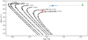 |
Fig. 10. Evolution of the hot component of Gaia18aen in the HR diagram throughout its outburst. The green symbol corresponds to the optical maximum; the blue and orange symbols represent the values calculated using the datasets obtained 20 and 81 d after the outburst maximum, respectively. The dotted solid curves are steady models of Nomoto et al. (2007). |
The high luminosity and temperature indicate that Gaia18aen could be detectable in soft X-rays. On the other hand, the object is highly reddened and therefore the source has probably not been reported in X-rays yet.
4. Conclusions
In this work, we analyzed the photometric and spectroscopic observations of Gaia18aen, a transient detected by the Gaia satellite at the beginning of the year 2018. Our main findings are as follows:
-
Gaia18aen is a classical symbiotic star, fulfilling the traditional criteria for symbiotic stars. Raman scattered O VI lines are observed in its spectra outside the outbursts.
-
The system is located at the distance ∼6 kpc, 0.2 kpc from the central disk surface.
-
The cool component of this symbiotic binary is an M giant with Teff ∼ 3500 K of a slightly super-solar metallicity, [Fe/H] = +0.25 dex, with a radius of ∼230 R⊙. Its luminosity, L ∼ 7400 L⊙, makes this system one of the brightest symbiotic giants. The NIR spectrum and IR photometry from 2MASS and WISE are consistent with a non-dusty S-type symbiotic star.
-
The system experienced an outburst of about 3.3 mag in 2018, followed by re-brightening detected approximately after 100, 240, and 350 d. At least the first outburst was accompanied by the increase of the hot component luminosity (Lh ∼ 28 000 L⊙ at the optical maximum) and the decrease in temperature (A or F-type photosphere), in comparison with temperature ∼68 kK and ∼135 kK, and luminosity of ∼26 600 and 5500 L⊙, corresponding to the observations obtained 20 and 81 d after the optical maximum, respectively.
-
The outburst was accompanied by the changes in emission spectral lines typical for classical symbiotic stars. In outburst, higher fluxes of lower ionization lines of H I and He I have been observed, together with the decrease of intensity of high ionization lines of He II, [O III], [Fe VII], and O VI.
-
The quiescent light curves of the object are characterized by a periodicity of approximately 487 d, which we tentatively attributed to the orbital modulation. The scatter in the light curves might be caused by stellar pulsations of the red giant with a period of 50−200 d, which are typical for cool components in S-type symbiotics.
These findings make Gaia18aen the first symbiotic star discovered by the Gaia satellite. This discovery proves the fact, that besides the astrometric mission of the Gaia, its repeated and high-precision observations can serve also as an photometric transient survey.
Acknowledgments
The research of JaM was supported by the Charles University, project GA UK No. 890120 and by internal grant VVGS-PF-2019-1047 of the Faculty of Science, P. J. Šafárik University in Košice. This research has been partly founded by the National Science Centre, Poland, through grant OPUS 2017/27/B/ST9/01940 to JM. MG and JS are supported by the Polish NCN MAESTRO grant 2014/14/A/ST9/00121. CG has been financed by Polish NCN grant SONATA No. DEC-2015/19/D/ST9/02974. ŁW acknowledges support from the Polish NCN grant Daina No. 2017/27/L/ST9/03221. ŁW and PZ acknowledge support from EC Horizon 2020 grant No 730890 (OPTICON). The Faulkes Telescope Project is an education partner of Las Cumbres Observatory (LCO). The Faulkes Telescopes are maintained and operated by LCO. We thank David Asher of Armagh Observatory for collecting part of the data. We acknowledge the use of the Cambridge Photometric Calibration Server (http://gsaweb.ast.cam.ac.uk/followup), developed by Sergey Koposov and maintained by Łukasz Wyrzykowski, Arancha Delgado, Paweł Zieliński, funded by the European Union’s Horizon 2020 research and innovation programme under grant agreement No 730890 (OPTICON). This work has made use of data from the European Space Agency (ESA) mission Gaia (https://www.cosmos.esa.int/gaia), processed by the Gaia Data Processing and Analysis Consortium (DPAC, https://www.cosmos.esa.int/web/gaia/dpac/consortium). Funding for the DPAC has been provided by national institutions, in particular the institutions participating in the Gaia Multilateral Agreement; the use of the SIMBAD and VIZIER databases, operated at CDS, Strasbourg, France; the data products from the Two Micron All Sky Survey, which is a joint project of the University of Massachusetts and the Infrared Processing and Analysis Center/California Institute of Technology, funded by the National Aeronautics and Space Administration and the National Science Foundation and the data products from the Wide-field Infrared Survey Explorer, which is a joint project of the University of California, Los Angeles, and the Jet Propulsion Laboratory/California Institute of Technology, funded by the National Aeronautics and Space Administration.
References
- Allard, F., Homeier, D., & Freytag, B. 2011, ASP Conf. Ser., 448, 91 [NASA ADS] [Google Scholar]
- Asplund, M., Grevesse, N., Sauval, A. J., & Scott, P. 2009, ARA&A, 47, 481 [NASA ADS] [CrossRef] [Google Scholar]
- Bailer-Jones, C. A. L., Rybizki, J., Fouesneau, M., Mantelet, G., & Andrae, R. 2018, AJ, 156, 58 [NASA ADS] [CrossRef] [Google Scholar]
- Belczyński, K., Mikołajewska, J., Munari, U., Ivison, R. J., & Friedjung, M. 2000, A&AS, 146, 407 [NASA ADS] [CrossRef] [EDP Sciences] [Google Scholar]
- Bensby, T., Feltzing, S., & Oey, M. S. 2014, A&A, 562, A71 [NASA ADS] [CrossRef] [EDP Sciences] [Google Scholar]
- Cardelli, J. A., Clayton, G. C., & Mathis, J. S. 1989, ApJ, 345, 245 [NASA ADS] [CrossRef] [Google Scholar]
- Cox, D. P., & Mathews, W. G. 1969, ApJ, 155, 859 [NASA ADS] [CrossRef] [Google Scholar]
- Delgado, A., Harrison, D., Hodgkin, S., et al. 2018, Transient Name Server Discovery Report, No. 2018-84 [Google Scholar]
- Gaia Collaboration (Brown, A. G. A., et al.) 2018, A&A, 616, A1 [NASA ADS] [CrossRef] [EDP Sciences] [Google Scholar]
- Gałan, C., Mikołajewska, J., Hinkle, K. H., & Joyce, R. R. 2017, MNRAS, 466, 2194 [NASA ADS] [CrossRef] [Google Scholar]
- Gonçalves, D. R., Magrini, L., Munari, U., Corradi, R. L. M., & Costa, R. D. D. 2008, MNRAS, 391, L84 [NASA ADS] [CrossRef] [Google Scholar]
- Gonçalves, D. R., Magrini, L., Martins, L. P., Teodorescu, A. M., & Quireza, C. 2012, MNRAS, 419, 854 [NASA ADS] [CrossRef] [Google Scholar]
- Gonçalves, D. R., Magrini, L., de la Rosa, I. G., & Akras, S. 2015, MNRAS, 447, 993 [NASA ADS] [CrossRef] [Google Scholar]
- González-Riestra, R., Viotti, R., Iijima, T., & Greiner, J. 1999, A&A, 347, 478 [NASA ADS] [Google Scholar]
- Goorvitch, D. 1994, ApJS, 95, 535 [NASA ADS] [CrossRef] [Google Scholar]
- Gromadzki, M., Mikołajewska, J., & Soszyński, I. 2013, Acta Astron., 63, 405 [NASA ADS] [Google Scholar]
- Gustafsson, B., Edvardsson, B., Eriksson, K., et al. 2008, A&A, 486, 951 [NASA ADS] [CrossRef] [EDP Sciences] [Google Scholar]
- Haas, M., Hackstein, M., Ramolla, M., et al. 2012, Astron. Nachr., 333, 706 [NASA ADS] [Google Scholar]
- Hackstein, M., Fein, C., Haas, M., et al. 2015, Astron. Nachr., 336, 590 [NASA ADS] [CrossRef] [Google Scholar]
- Hillman, Y., Prialnik, D., Kovetz, A., Shara, M. M., & Neill, J. D. 2014, MNRAS, 437, 1962 [CrossRef] [Google Scholar]
- Hodgkin, S. T., Wyrzykowski, Ł., Blagorodnova, N., & Koposov, S. 2013, Philos. Trans. R. Soc. London Ser. A, 371, 20120239 [Google Scholar]
- Iijima, T. 1981, Photometric and Spectroscopic Binary Systems (Dordrecht: Kluwer), 517 [CrossRef] [Google Scholar]
- Iłkiewicz, K., & Mikołajewska, J. 2017, A&A, 606, A110 [NASA ADS] [CrossRef] [EDP Sciences] [Google Scholar]
- Iłkiewicz, K., Mikołajewska, J., & Shara, M. M. 2018a, ApJ, submitted [arXiv:1811.06696] [Google Scholar]
- Iłkiewicz, K., Mikołajewska, J., Miszalski, B., Kozłowski, S., & Udalski, A. 2018b, MNRAS, 476, 2605 [NASA ADS] [CrossRef] [Google Scholar]
- Kausch, W., Noll, S., Smette, A., et al. 2015, A&A, 576, A78 [NASA ADS] [CrossRef] [EDP Sciences] [Google Scholar]
- Kenyon, S. J. 1986, The Symbiotic Stars (Cambridge: University Press) [CrossRef] [Google Scholar]
- Kenyon, S. J., Oliversen, N. A., Mikołajewska, J., et al. 1991, AJ, 101, 637 [NASA ADS] [CrossRef] [Google Scholar]
- Kniazev, A. Y., Väisänen, P., Whitelock, P. A., et al. 2009, MNRAS, 395, 1121 [NASA ADS] [CrossRef] [Google Scholar]
- Kochanek, C. S., Shappee, B. J., Stanek, K. Z., et al. 2017, PASP, 129, 104502 [Google Scholar]
- Kolb, U., Brodeur, M., Braithwaite, N., & Minocha, S. 2018, Robotic Telescope, Student Research and Education Proceedings, 1, 127 [CrossRef] [Google Scholar]
- Kruszyńska, K., Gromadzki, M., Wyrzykowski, Ł., et al. 2018, ATel, 11634, 1 [Google Scholar]
- Kupka, F., Piskunov, N., Ryabchikova, T. A., Stempels, H. C., & Weiss, W. W. 1999, A&AS, 138, 119 [NASA ADS] [CrossRef] [EDP Sciences] [MathSciNet] [PubMed] [Google Scholar]
- Leedjärv, L., Gális, R., Hric, L., Merc, J., & Burmeister, M. 2016, MNRAS, 456, 2558 [CrossRef] [Google Scholar]
- Merc, J., Gális, R., & Teyssier, F. 2019, Contrib. Astron. Obs. Skaln. Pleso, 49, 228 [Google Scholar]
- Mikołajewska, J. 2003, ASP Conf. Ser., 303, 9 [NASA ADS] [Google Scholar]
- Mikołajewska, J. 2007, Balt. Astron., 16, 1 [Google Scholar]
- Mikołajewska, J. 2010, ArXiv e-prints [arXiv:1011.5657] [Google Scholar]
- Mikołajewska, J. 2012, Balt. Astron., 21, 5 [NASA ADS] [Google Scholar]
- Mikołajewska, J., & Kenyon, S. J. 1992, AJ, 103, 579 [NASA ADS] [CrossRef] [Google Scholar]
- Mikołajewska, J., & Kenyon, S. J. 1996, AJ, 112, 1659 [NASA ADS] [CrossRef] [Google Scholar]
- Mikołajewska, J., Kenyon, S. J., Mikolajewski, M., Garcia, M. R., & Polidan, R. S. 1995, AJ, 109, 1289 [NASA ADS] [CrossRef] [Google Scholar]
- Mikołajewska, J., Acker, A., & Stenholm, B. 1997, A&A, 327, 191 [Google Scholar]
- Mikołajewska, J., Caldwell, N., & Shara, M. M. 2014, MNRAS, 444, 586 [NASA ADS] [CrossRef] [Google Scholar]
- Mikołajewska, J., Shara, M. M., Caldwell, N., Iłkiewicz, K., & Zurek, D. 2017, MNRAS, 465, 1699 [NASA ADS] [CrossRef] [Google Scholar]
- Miszalski, B., & Mikołajewska, J. 2014, MNRAS, 440, 1410 [NASA ADS] [CrossRef] [Google Scholar]
- Miszalski, B., Mikołajewska, J., & Udalski, A. 2013, MNRAS, 432, 3186 [NASA ADS] [CrossRef] [Google Scholar]
- Munari, U. 2019, Camb. Astrophys. Ser., 54, 77 [Google Scholar]
- Murset, U., & Nussbaumer, H. 1994, A&A, 282, 586 [Google Scholar]
- Netzer, H. 1975, MNRAS, 171, 395 [NASA ADS] [Google Scholar]
- Nomoto, K., Saio, H., Kato, M., & Hachisu, I. 2007, ApJ, 663, 1269 [NASA ADS] [CrossRef] [Google Scholar]
- Piascik, A. S., Steele, I. A., Bates, S. D., et al. 2014, Proc. SPIE, 9147, 91478H [Google Scholar]
- Proga, D., Mikołajewska, J., & Kenyon, S. J. 1994, MNRAS, 268, 213 [NASA ADS] [CrossRef] [Google Scholar]
- Rodríguez-Flores, E. R., Corradi, R. L. M., Mampaso, A., et al. 2014, A&A, 567, A49 [NASA ADS] [CrossRef] [EDP Sciences] [Google Scholar]
- Schlafly, E. F., & Finkbeiner, D. P. 2011, ApJ, 737, 103 [NASA ADS] [CrossRef] [Google Scholar]
- Schlegel, D. J., Finkbeiner, D. P., & Davis, M. 1998, ApJ, 500, 525 [NASA ADS] [CrossRef] [Google Scholar]
- Schmidt, M. R., Začs, L., Mikołajewska, J., & Hinkle, K. H. 2006, A&A, 446, 603 [NASA ADS] [CrossRef] [EDP Sciences] [Google Scholar]
- Scott, P., Asplund, M., Grevesse, N., Bergemann, M., & Sauval, A. J. 2015a, A&A, 573, A26 [NASA ADS] [CrossRef] [EDP Sciences] [Google Scholar]
- Scott, P., Grevesse, N., Asplund, M., et al. 2015b, A&A, 573, A25 [NASA ADS] [CrossRef] [EDP Sciences] [Google Scholar]
- Shappee, B. J., Prieto, J. L., Grupe, D., et al. 2014, ApJ, 788, 48 [NASA ADS] [CrossRef] [Google Scholar]
- Siebenmorgen, R., Krełowski, J., Smoker, J., Galazutdinov, G., & Bagnulo, S. 2020, A&A, 641, A35 [CrossRef] [EDP Sciences] [Google Scholar]
- Skowron, D. M., Skowron, J., Mróz, P., et al. 2019, Science, 365, 478 [Google Scholar]
- Skrutskie, M. F., Cutri, R. M., Stiening, R., et al. 2006, AJ, 131, 1163 [NASA ADS] [CrossRef] [Google Scholar]
- Smette, A., Sana, H., Noll, S., et al. 2015, A&A, 576, A77 [NASA ADS] [CrossRef] [EDP Sciences] [Google Scholar]
- Sneden, C., Lucatello, S., Ram, R. S., Brooke, J. S. A., & Bernath, P. 2014, ApJS, 214, 26 [Google Scholar]
- Steele, I. A., Smith, R. J., Rees, P. C., et al. 2004, SPIE Conf. Ser., 5489, 679 [Google Scholar]
- Tonry, J. L., Denneau, L., Heinze, A. N., et al. 2018, PASP, 130, 064505 [NASA ADS] [CrossRef] [Google Scholar]
- Udalski, A., Szymański, M. K., & Szymański, G. 2015, Acta Astron., 65, 1 [NASA ADS] [Google Scholar]
- Ulmer-Moll, S., Figueira, P., Neal, J. J., Santos, N. C., & Bonnefoy, M. 2019, A&A, 621, A79 [NASA ADS] [CrossRef] [EDP Sciences] [Google Scholar]
- Vernet, J., Dekker, H., D’Odorico, S., et al. 2011, A&A, 536, A105 [NASA ADS] [CrossRef] [EDP Sciences] [Google Scholar]
- Wray, J. D. 1966, PhD Thesis, Northwestern University, USA [Google Scholar]
- Wright, E. L., Eisenhardt, P. R. M., Mainzer, A. K., et al. 2010, AJ, 140, 1868 [Google Scholar]
- Wyrzykowski, Ł., & Hodgkin, S. 2012, IAU Symp., 285, 425 [NASA ADS] [Google Scholar]
- Wyrzykowski, Ł., Hodgkin, S., & Blagorodnova, N. 2014, Gaia-FUN-SSO-3, 31 [Google Scholar]
- Wyrzykowski, Ł., Mróz, P., Rybicki, K. A., et al. 2020, A&A, 633, A98 [NASA ADS] [CrossRef] [EDP Sciences] [Google Scholar]
- Zieliński, P., Wyrzykowski, Ł., Rybicki, K., et al. 2019, Contrib. Astron. Obs. Skaln. Pleso, 49, 125 [Google Scholar]
- Zieliński, P., Wyrzykowski, Ł., Mikolajczyk, P., Rybicki, K., & Kolaczkowski, Z. 2020, ArXiv e-prints [arXiv:2006.05160] [Google Scholar]
Appendix A: Photometrical observation
Photometrical observations of Gaia18aen.
All Tables
Positions, radial velocities, and fluxes of identified emission lines in the VLT/X-shooter spectrum of Gaia18aen obtained on March 22, 2018.
Final values of abundances obtained from K-band region together with the formal fitting errors and 12C/13C isotopic ratio.
All Figures
|
Fig. 1. VLT/X-shooter spectrum of Gaia18aen obtained on March 22, 2018. Upper panel: spectrum in the UBV arm, middle panel: in VIS arm, and bottom panel: spectrum obtained in the NIR arm. The spectrum was corrected for the telluric features (see the text). |
| In the text | |
|
Fig. 2. Comparison of the two spectra of Gaia18aen obtained on January 20 and March 22, 2018 together with the identification of the major emission lines observed. |
| In the text | |
|
Fig. 3. Line profiles of the Na I D1 (black) and Na I D2 (red). |
| In the text | |
|
Fig. 4. Surface of χ2 in function of Teff and [M/H] parameters. Two selected cases are distinguished with red (the best match) and magenta (with atmospheric parameters close to those obtained via spectral synthesis fit; see Figs. 5 and 6). |
| In the text | |
|
Fig. 5. Comparison of the VLT/X-shooter spectrum and the synthetic model. The VLT/X-shooter spectrum (black line) de-reddened by EB − V = 1.25 is compared with the synthetic model (magenta) corresponding to the following atmospheric parameters: Teff = 3500 K, log g = 0.0, [M/H] = 0.0, and [α/H] = 0.0. The residuals – observations minus calculations – are shown at the bottom with gray line. The spectra were normalized to the flux level at the narrow range (50 Å) centered at 22 155 Å. The scale factor is Sf = Fobs/Fmodel = 7.7 × 10⁻¹⁹. |
| In the text | |
|
Fig. 6. VLT/X-shooter spectrum of Gaia18aen (black line) and synthetic spectrum (magenta line) calculated using the final abundances (Table 4). |
| In the text | |
|
Fig. 7. Light curves of Gaia18aen. Individual light curves in various filters were shifted to the level in the OGLE V filter for clarity; values of shifts are shown in the figure legend. Different colors denote different filters. |
| In the text | |
|
Fig. 8. Outbursts of Gaia18aen. The colors are the same as in Fig. 7. The vertical dotted lines indicate the individual brightenings (denoted by numbers 0−5). The arrows show the times when the two spectra were obtained. |
| In the text | |
|
Fig. 9. Light curves in selected filters phased with the period of P = 486.9 d. Individual datasets were shifted to the level in the OGLE I filter. |
| In the text | |
|
Fig. 10. Evolution of the hot component of Gaia18aen in the HR diagram throughout its outburst. The green symbol corresponds to the optical maximum; the blue and orange symbols represent the values calculated using the datasets obtained 20 and 81 d after the outburst maximum, respectively. The dotted solid curves are steady models of Nomoto et al. (2007). |
| In the text | |
Current usage metrics show cumulative count of Article Views (full-text article views including HTML views, PDF and ePub downloads, according to the available data) and Abstracts Views on Vision4Press platform.
Data correspond to usage on the plateform after 2015. The current usage metrics is available 48-96 hours after online publication and is updated daily on week days.
Initial download of the metrics may take a while.