| Issue |
A&A
Volume 644, December 2020
|
|
|---|---|---|
| Article Number | A134 | |
| Number of page(s) | 22 | |
| Section | Extragalactic astronomy | |
| DOI | https://doi.org/10.1051/0004-6361/202039029 | |
| Published online | 11 December 2020 | |
The COld STream finder Algorithm (COSTA)
Searching for kinematical substructures in the phase space of discrete tracers
1
University of Naples Federico II, C.U. Monte SantAngelo, Via Cinthia, 80126 Naples, Italy
2
School of Physics and Astronomy, Sun Yat-sen University Zhuhai Campus, 2 Daxue Road, Tangjia, Zhuhai, Guangdong 519082, PR China
e-mail: This email address is being protected from spambots. You need JavaScript enabled to view it.
3
Sub-Department of Astrophysics, Department of Physics, University of Oxford, Denys Wilkinson Building, Keble Road, Oxford OX1 3RH, UK
4
INAF-Osservatorio Astronomico di Capodimonte, Via Moiariello 16, 80131 Naples, Italy
Received:
24
July
2020
Accepted:
2
October
2020
Abstract
Context. We present the COld STream finder Algorithm (COSTA), a novel algorithm used to search for cold kinematical substructures in the phase space of planetary nebulae (PNe) and globular clusters (GCs) in the halos of massive galaxies and intracluster regions.
Aims. The aim of COSTA is to detect small, low-velocity-dispersion streams, such as the ones produced in recent interactions of dwarf galaxies with the halos of more massive galaxies, including the ones sitting in the central regions of rich galaxy clusters.
Methods. We based COSTA on a deep friend-of-friend procedure that isolates groups of N particles with low velocity dispersion (between 10 km s−1 and ∼100 km s−1) using an iterative (n) sigma-clipping on a defined number of (k) neighbor particles. The algorithm has three parameters (k − n − N), plus a velocity dispersion cut-off that defines the “coldness” of the stream, which are set using Monte Carlo realizations of the sample in question.
Results. In this paper, we show the ability of COSTA to recover simulated streams on mock datasets of discrete kinematical tracers of different sizes and measurement errors, from publicly available hydrodynamical simulations. We also show the best algorithm setup for realistically locating streams in the core of the Fornax cluster, for future applications of COSTA to real populations of PNe and GCs.
Conclusions. Finally, COSTA can be adapted to many situations in finding small substructures in the phase space of a limited sample of discrete tracers, provided that the algorithm is trained on realistic mock observations reproducing the specific dataset under examination.
Key words: galaxies: kinematics and dynamics / galaxies: halos / galaxies: interactions / techniques: radial velocities
© ESO 2020
1. Introduction
In the hierarchical formation scenario, massive structures grow in a bottom-up manner assembling mass via the merging of many smaller systems (White & Rees 1978). This is an ongoing process, as demonstrated by cosmological simulations (Naab et al. 2007, 2009; Cooper et al. 2010; Oser et al. 2010, 2012).
In the Local Group, the accretion of smaller building blocks has been observed in the last decades (Ibata et al. 1994, 1995; Yanny et al. 2000) in the form of dwarf debris (Ibata et al. 2001a; Majewski et al. 2003). In denser environments, like galaxy groups or clusters, this mechanism is enhanced because of the whirl of encounters and collisions, leading to the formation of an extended halo around the central galaxy (e.g., Cooper et al. 2010). Central dominant (cD) galaxies in the innermost region of the richest clusters are the archetypes of this scenario, with exceptional merging histories (e.g., Ruszkowski & Springel 2009; Weinzirl et al. 2014; Iodice et al. 2016). The remarkable large stellar masses of cDs (M⋆ ≥ 1012 M⊙) are well explained in the hierarchical scenario, as the mass assembly is expected to happen either through the tidal stripping of stars and globular clusters from their satellite or dwarfs (Gallagher & Ostriker 1972; Moore et al. 1996; Gregg & West 1998; Willman et al. 2004; Read et al. 2006), or through major mergers with other bright galaxies or minor ones in which the cD “eats” smaller systems (Ostriker & Tremaine 1975; White 1976; Malumuth & Richstone 1984; Merritt 1985; Liu et al. 2015; Nipoti 2017). In particular, numerical simulations and semi-analytic models have demonstrated that the bulk of their accreted mass and extended halos was built up in the last few Gyr, especially through minor merger events (e.g., De Lucia & Blaizot 2007; Amorisco 2019). As all these processes are expected to still be in action, one can search for observational signatures of such events in the cluster core, either with the deep photometry (see e.g., Mihos et al. 2005, 2017; Iodice et al. 2017) or in the kinematics of stars and other kinematical tracers such as planetary nebulae and globular clusters (e.g., Napolitano et al. 2003; Romanowsky et al. 2012; Longobardi et al. 2015; Spiniello et al. 2018; Pota et al. 2018; Amorisco 2019). Hence, stellar substructures in galaxy halos (and beyond, i.e., in the intracluster regions), in the form of debris of past or recent merger events, are invaluable pieces of information for studying the mechanisms that supply mass in the assembly history of galaxies in dense environments.
In recent years, the study of the signature of minor mergers in the local Universe, like halo shells and ripples, tidal streams, or other stellar substructures, has become an important tool for probing the assembly histories of galaxies (e.g., Helmi et al. 1999; Ibata et al. 2001b; Belokurov et al. 2006; Tal et al. 2009; Martínez-Delgado et al. 2010; Cooper et al. 2011; Mouhcine et al. 2011; Xue et al. 2011; Bate et al. 2014). The number of newly discovered stellar streams and other substructures in the halos of nearby galaxies has dramatically increased, showing that remnants of merger events could be almost ubiquitous. Among the most important examples, we can count the Sagittarius Stream in the Milky Way (Ibata et al. 1997, 2001c; Majewski et al. 2003) and many other substructures detected around M 31 (Andromeda galaxy; e.g. McConnachie et al. 2009; Ibata et al. 2001d).
Early investigations of such substructures were based on photometric observations. However, this approach is challenging due to the faint surface brightness of the remnants, typically below μ ∼ 27 mag arcsec−2. This implies that only the brightest substructures are generally detected, while most of the accreted mass provided by the fainter events, which generally have a surface brightness of the order of 30 mag arcsec−2 or below (Cooper et al. 2010), remain hidden in the central galaxy background.
In the last few years, deeper and more accurate spectroscopy has made it possible to include kinematic information relating to the debris, in order to go beyond the purely photometric studies and look into the phase space (projected positions and line-of-sight (LOS) velocities) to search for the typical signatures expected in these interactions (e.g., Johnston et al. 2008; Romanowsky et al. 2012). Within the Local Group, these substructures can be studied using individual stars (e.g., Koch et al. 2008; Gilbert & Vacca 2009; Starkenburg et al. 2009; Xue et al. 2011; Belokurov & Koposov 2016). Outside the Local Group, stars cannot be resolved and other kinematical tracers have to be used. Planetary nebulae (PNe) and globular clusters (GCs) are suitable tracers of this kind as they are observable at large distances from the galaxy centers (Durrell et al. 2003; Merrett et al. 2003; Douglas et al. 2007; Shih & Méndez 2010; Cortesi et al. 2011; Richtler et al. 2011) and their velocities can be measured with good precision in nearby galaxies and galaxy clusters. They represent a viable alternative for studying the outskirts of galaxies where it is very hard to measure stellar absorption lines and thus obtain kinematical information from the integrated light (PNe: Hui et al. 1995; Napolitano et al. 2002, 2009; Romanowsky et al. 2003, 2009, 2012; De Lorenzi et al. 2009; Coccato et al. 2009; Richtler et al. 2011; Forbes et al. 2011; Pota et al. 2013, 2018; Longobardi et al. 2015, 2018; Hartke et al. 2018; Spiniello et al. 2018; GCs: Cóté et al. 2003; Schuberth et al. 2010; Woodley & Harris 2011; Foster et al. 2014; Veljanoski & Helmi 2016). The combined information of position and velocity of tracers in the halo regions of galaxies allows us to study substructures in the tracer phase space, where they have not yet fully mixed due to the long dynamical times (Napolitano et al. 2003; Arnaboldi et al. 2004, 2012; Bullock & Johnston 2005; Coccato et al. 2013; Longobardi et al. 2015).
Historically, the methods adopted to search for streams have been very empirical and have lacked well-encoded (objective) criteria to systematize the search for streams in the full phase space. Only recently, a big effort has been made to develop stream-locator algorithms suitable for different datasets. For the Milky Way, Malhan & Ibata (2018) implemented STREAMFINDER, with the aim of unveiling dynamically cold structures in the 6D phase space, by taking advantage of the Gaia space mission data. This code looks for a handful of particles (as few as 15 members) that lie along a similar orbit, allowing them to detect tiny and ultra-faint streams in the Galactic Halo. Other algorithms have been focused on the automatic search for tidal structures, like shells or ridges, in deep images (e.g., Kado-Fong et al. 2018; Hendel et al. 2019). Such approaches are more directed toward large samples of galaxies to build statistically significant samples of stream features, but they do not rely on kinematics. As stated before, this is not ideal when looking for low-surface-brightness tidal features, which we expect to be those originating from minor mergers (see Cooper et al. 2010).
In this context, we present the COld STream finder Algorithm (COSTA), a new method used to search for candidate cold substructures that can be interpreted as signatures of recent or past interaction between a main galaxy and the dwarf galaxies surrounding it. COSTA aims to fill the gap left by the above algorithms, introducing a method that relies on kinematics (namely a reduced 3D phase space of projected positions and LOS velocities), which can reveal streams even beyond the Local Group and can still be applied to large galaxy samples but below the detection limits imposed by the photometry.
We introduce the basic statistical methods that allow the identification of cold kinematical substructures made of a few tens of particles, compatible with what is expected for faint streams around galaxies. The method is based on a k-nearest-neighbors (KNN) approach, which groups nearby particles in 2D positions and in velocity to find coherent kinematic substructures. The algorithm is general and can be applied to any nearby stellar system, either galaxies or galaxy clusters cores (where large galaxy haloes and intracluster light concentration reside).
As a template of this latter example to show the potential of the method, we discuss here the specific case of the Fornax cluster core. The Fornax cluster is particularly suitable for such a test as different studies have provided evidence of recent galaxy interactions (e.g., D’Abrusco et al. 2016; Iodice et al. 2017; Spiniello et al. 2018; Sheardown et al. 2018). This complexity represents a challenging test bench for the algorithm. For this paper, we used a mock observation of the Fornax cluster to assess the reliability of the method and to demonstrate how to set up the best parameters in a real case. In a companion paper (in preparation), we will then apply COSTA to identify real streams of GCs and PNe from the Fornax VST Spectroscopic Survey (FVSS; Pota et al. 2018; Spiniello et al. 2018; hereafter P+18 and S+18, respectively).
The paper is structured as follows: in Sect. 2, we present a brief description of the algorithm. In Sects. 3 and 4, we test it on hydrodynamical simulations of pair interacting galaxies and on Monte Carlo simulations of the Fornax cluster core, respectively. Finally, in Sect. 5, we draw our conclusions.
2. The COld STream finder Algorithm
In this section, we introduce COSTA, which is intended to detect cold substructures in the reduced phase space (position on the sky and radial velocity) of discrete tracers. In order to find cold substructures that are correlated both in position and in velocity, we implemented an algorithm that looks for points close both in the RA/Dec position space and in the reduced phase space (velocity vs. radius). The method relies on a pseudo-KNN method based on a deep friend-of-friend algorithm that isolates groups of (N) particles with a small velocity dispersion (σcut, chosen between 10 km s−1 and ∼100 km s−1).
The main difficulty lies in efficiently detecting particles belonging to the stream, which should preserve the low velocity dispersion of the dwarf progenitor while they are moving in regions where the potential of the cluster rules, and the local velocity dispersion is that of the cluster (i.e., up to 50 times larger than typical dwarf-like velocity dispersions). To do that, for each particle, the algorithm starts performing an iterated sigma clipping on a number (k) of neighbors. In particular, it removes all the particles with a velocity outside the interval [ ,
,  ], where
  and σ are the mean velocity and the velocity dispersion of the k particles, and n is the sigma clipping value. As a proxy for the velocity dispersion, we used the standard deviation of the individual velocities (see Sect. 3.2). The algorithm iterates the procedure, with the mean velocity and velocity dispersion of the remaining particles, until there are no outliers to be clipped. Once the procedure is over, the algorithm selects all structures in the position and velocity space with a minimal number (Nmin) of particles.
To define the maximum velocity dispersion acceptable for a given substructure to be considered cold, COSTA uses another parameter: the cut-off velocity dispersion, σcut. We fine-tuned our algorithm to locate cold streams originating from the interaction of dwarf galaxies with the cluster. In fact, we expect that dwarf disruption is the main mechanism contributing to the later formed intracluster stellar population and the assembly of large stellar halos around galaxies. Hence, we allow for σcut values ranging from 10 to ∼100 km s−1, based on the typical dwarf-like dispersion values found in the Coma cluster (Kourkchi et al. 2012).
The final COSTA output is a list of substructures with low velocity dispersion, below the fixed threshold, σcut. We note here that more massive galaxies would produce more diffuse substructures, due to a higher velocity dispersion and larger sizes. These would be harder to “filter” in the phase space, as they would be more mixed in the warm halo environment.
Thus, to summarize, the COSTA algorithm has a total of three parameters (k, n, and Nmin) for any given (upper) dispersion threshold, σcut, which needs to be properly chosen to maximize the number of real cold substructures (completeness) and minimize the number of spurious detections (purity), caused by the intrinsic stochastic nature of the velocity field of hot systems. For this purpose, one can use Monte Carlo realizations of the specific sample under examination.
Our approach has the advantage of being able to refine the selection of coherent spatial and velocity substructures, but it has the disadvantage of being biased toward round geometries. In fact, the algorithm is based on a simple metric that uses the distances from every single particle. This reduces the chance of identifying chain-like structures, which are expected in elongated streams. To remove this bias, we added a second stage to COSTA, at which we verify if some of the groups belong to a single structure. In particular, we define two or more groups belonging to a single structure if they show at least one common particle and their velocity dispersion values differ by less than their uncertainties.
To demonstrate that it is possible to identify regions in this parameter space that can reliably detect streams with an acceptable fraction of false positives, we first tested the algorithm on a simulated sample from the publicly available hydrodynamical GalMer simulations (Chilingarian et al. 2010), and then train the algorithm to search for stellar streams in the Fornax cluster core. The results of these tests are presented in the next sections.
3. Testing COSTA on hydrodynamical simulations
We used a suite of publicly available simulations, the GalMer database (Chilingarian et al. 2010), to test the ability of our algorithm to recover streams originating from a dwarf when passing close to a giant galaxy. The simulated data cubes are needed to test the algorithm self-consistently.
We first defined the series of (k, n, Nmin, and σcut) setups that minimize false detections, and then applied them to find the stream. Finally, we checked how meaningful the recovered properties (e.g., mean velocity, local velocity dispersion, and fraction of particles) were with respect to the intrinsic property of the stream. At this point, we were interested in verifying whether for a given stream a series of parameter setups would allow COSTA to find it and how these might change as a function of the observational conditions (i.e., measurement errors and total number of particles).
3.1. The GalMer Simulations
The GalMer simulations are based on a tree-smoothed particle hydrodynamics (SPH) code, in which gravitational forces are calculated using a hierarchical tree method (Barnes & Hut 1986) and gas evolution is followed by means of SPH (Lucy 1977; Gingold & Monaghan 1982). Dark matter particles and baryon particles both have masses of ∼105 M⊙, while the softening lengths are ϵ = 280 pc for giant-giant interactions, and ϵ = 200 pc for giant-intermediate and giant-dwarf runs. This gives an appropriate mass and spatial resolution to trace low-mass and low-surface-brightness substructures. The typical mass residing in stellar streams stripped by the dwarf during its interaction with the large galaxy is of the order of 10% of its mass; thus, given the typical GC- and PN-specific number densities (the number of particles per unit of luminosity), the stream is fairly sampled with a few tens of and up to a hundred tracers (e.g., GCs and PNe together). We simulated different depths of our observational setup by assuming different numbers of stellar particles expected to populate the stream.
The advantage of testing the algorithm on simulations is that we can separate the particles belonging to the dwarf galaxy from the ones belonging to the target system. We can, therefore, characterize the phase space of both the galaxy target and streams produced in the fly-by of the dwarf galaxy through the central galaxy halo.
The GalMer database1 provides about 1019 simulations of colliding galaxies and more than 70 000 snapshots showing the development of these interactions up to 3 Gyr from the beginning of the encounter with a bin interval, for each snapshot, of 50 Myr. From the whole database, we focused on two encounter configurations: (1) the one between a giant elliptical galaxy, gE0, and a dwarf E0 galaxy, dE0, with a mass ratio of 1:10 (the minimum found in the database for all simulations); and (2) the one between a giant Sa galaxy, gSa, and a dwarf S0 galaxy, dS0, also with a mass ratio 1:10. Table 1 shows the parameters of the four galaxies. We need to point out that a mass ratio of 1:10 is not optimal for generalizing the results because a wider population of systems, also with lower mass ratios, exist in real cases. As we show later, however, this is a conservative starting point as our algorithm is more efficient in detecting groups in phase spaces, which are generally much colder than the surrounding environment. Hence, the differences in velocity dispersion, which characterize the GalMer systems, are representative of extreme cases: if COSTA is able to detect substructures in these systems, then it will be even more successful in cases involving lower mass satellites.
Parameters of the selected galaxies in the galmer simulation.
We selected the gE0-dE0 and gSa-dS0 cases as realistic representations of the dynamics of a giant-dwarf encounter. In particular, the case of the gE0-dE0 is fairly representative of a typical encounter between a hot, high-dispersion system and a colder satellite, like the one happening in large galactic halos (see e.g., Cooper et al. 2010; Iodice et al. 2016). In both configurations, we chose an encounter with the satellite starting 100 kpc away, and falling toward the larger galaxy in a prograde orbit with an inclination of 33° and a pericentral distance of 16 kpc. We initially used a prograde orbit because this is expected to exchange a lower amount of energy and therefore to minimize the scatter of dwarf particles into warmer tails. However, since in the case of the gSa-dS0 encounter the dwarf and the giant stars were too mixed, for this latter case we also considered a retrograde encounter.
In Figs. 1 and 2, we show a few snapshots of the gE0-dE0 and gSa-dS0 encounters, respectively. The final configuration we adopt for our tests is shown in the central panel (encounter), while the other panels show different time snaps, each one spaced in time by 50 Myr, with the top-left corner temporarily located 200 Myr before the chosen configuration. The choice of the central configurations is motivated by the fact that the distance between the intruder and the giant galaxy is the shortest (as is evident from Figs. 1 and 2). This allows us to have a sufficient spatial mix of the two systems, and thus stress as much as possible the ability of COSTA to recover stream particles well embedded in high-density regions.
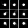 |
Fig. 1. Snapshots of gE0-dE0 encounter, from 1850 Myr (top left) up to 2250 Myr (bottom right) after the beginning of the simulation, and separated by steps of 50 Myr. To test COSTA, we use the configuration at the center of the image, which is temporarily located at 2050 Myr after the start of the encounter. |
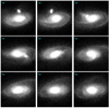 |
Fig. 2. Same as Fig. 1 but for gSa-dS0 interaction. These snapshots correspond to a time interval between 1650 Myr and 2050 Myr after the beginning of the simulation, with our test configuration (1850 Myr) at the center of the image. |
From the figures, it is also clear that the encounters start producing a stream-like structure from the first passage at a few tens of kpc. Particles belonging to the original stream become mixed after a few hundred Myr, but subsequent close passages produce even brighter streams. These latter ones remain visible and well separated from the background galaxy for hundreds of Myr. They later diffuse and mix with galaxy halo particles. This timescale is set by the specific dynamical time of the system in question, and this can be larger for hotter central systems and lower mass ratios. Unfortunately, the GalMer database does not provide lower mass ratios than the ones adopted here. Nevertheless, these examples allow us to test the ability of COSTA to find such cold streams as a function of a few observational parameters.
3.2. Running COSTA on GalMer simulations
In order to apply COSTA to GalMer simulations, we first needed to extract simulated 6D data cubes from the velocity field (i.e., RA, Dec, and a radial velocity) that mimics a typical observational situation. Then, COSTA can be applied to the mock velocity field to recover the cold substructures, together with their intrinsic kinematical parameters. We intended to test the possibility of identifying streams made of a few particles in velocity fields of different sizes. In particular, we tested the case of Npart = 2000, 1000, 500 extracted from the giant galaxy. These are typical numbers of test particles found in external galaxies, like PNe (Fornax cluster: ∼1500 PNe: Spiniello et al. 2018 and references therein; M 31, ∼2000 PNe: Merrett et al. 2006; NGC 5128, ∼1100 PNe: Peng et al. 2004; NGC 4374, ∼500 PNe: Napolitano et al. 2011) or globular clusters (Fornax cluster: ∼1000 GCs: Pota et al. 2018 and references therein; M 87, ∼500: Romanowsky et al. 2012). For the dwarfs, we instead considered Npart = 150, 75, 38, respectively (e.g., Fahrion et al. 2020). These numbers of particles were chosen to match with the expected particles observable from streams of surface brightness of the order of 28−30 mag arcsec−2 (see discussion below).
Finally, to test different observational conditions, we adopted three orders of measurement errors, Δv = 10, 20, 40 km s−1, for each of the three different selected encounters (i.e., gE0-dE0 and gSa-dS0 prograde/retrograde) by re-sampling the particle velocities with a Gaussian distribution centered on the particle velocity and with σ = Δv (vobs hereafter). These values are comparable to what is typically reached with mid and low spectral resolution. Measurement errors have the effect of diluting the observed velocity distribution of the cold substructure by increasing the observed squared velocity dispersion, that is,  , where σI idicates the intrinsic velocity dispersion of the stream and σobs the observed velocity dispersion.
In the following, we define the mean velocity and velocity dispersion of the detected substructures using a standard statistical definition (see also P+18):
 (1)
(1)
Hence, the larger the Δv, the greater the chance that a cold structure will become warm enough to skip the cold criterion on σcut, or that some of the particles are discarded by the sigma-clipping part of the algorithm. This would then leave too few particles to meet the minimum particle number (Nmin) limit, hence making COSTA lose good candidate streams.
3.3. Setting the reliability of COSTA
Before running COSTA to search for streams, we need to check whether and how often COSTA returns spurious detections. In the case of simulations, this is easily performed by running COSTA on the central galaxy particles only; these represent the smooth warm background in which streams must be found when the intruder is added.
For our analysis, we defined the following datasets: the white noise sample (WNS) includes RA, Dec, and vobs of the giant galaxy or cluster regions without any artificial stream added and the detection sample (DS) includes RA, Dec, and vobs of the full system including the WNS and the particles of the stream. We used the WNS to select those setups (i.e., combination of k, n, Nmin, and σcut) that have a reasonably low probability to find artificial detection and to be used to look for streams in the DS. A given setup that finds no spurious streams in the WNS has maximum “reliability”, which means that if it detects a stream in the DS then this is likely to be real. On the other hand, a setup that finds many spurious detections is highly unreliable and has to be discarded.
In order to have a statistical definition of the reliability of the setups in the k, n, Nmin, and σcut space, we used 100 different mock datasets randomly extracted from all particles in the simulations. We used different combinations of number of particles Npart and velocity errors Δv for each of the three encounters, and we present some representative cases here. Specifically, we discuss the cases where we randomly extracted 2000 particles with errors Δv = 10 and 40 km s−1; 1000 particles with Δv = 40 and 500 particles with Δv = 20 km s−1. For each case, we uniformly sampled the k, n, Nmin parameters’ space, for different σcut and ran COSTA with all the possible combinations of the free parameters selected in the following ranges:
-
k: from 10 to 30 with steps of 5.
-
n: from 1.3 to 3 with steps of 0.2−0.3.
-
Nmin: all values from 5 up to k.
-
σcut: from 10 to 80 km s−1 with steps of 5 km s−1.
For each combination of these parameters, we defined the reliability of the 100 random extractions as
 (2)
(2)
where Nspu is the number of times we obtain at least one spurious detection from COSTA.
We use 70% as the threshold for defining a reliable setup. This threshold is somehow arbitrary, as it might depend on the risk one is willing to take in considering a group of particles as a stream.
In principle, one should set the reliability toward 100%, to be sure that none of the detection is spurious. However, this could result in a too conservative choice that might cut all streams statistically closer to the white noise given by the background particles. For instance, the properties of streams with a low number of particles and/or too close to the σcut may be very close to the properties of the spurious detections, and thus would be filtered out by too-conservative thresholds. For this reason, we were motivated to choose a lower threshold that might provide greater completeness but less purity, due to the increased chance of finding spurious detections. Since the main scope of COSTA is to provide stream candidates that will then be confirmed with deeper observations, a fair amount of false detections are acceptable. We discuss the impact of the threshold in Sect. 3.6. Here we discuss the results for the gE0-dE0 and the gSa-dS0 encounters separately and in detail.
3.4. The case of the gE0-dE0 encounter
We first tested COSTA parameter combinations on the WNS to check which configurations produced spurious detections over 100 re-extractions of the same catalog, re-sampling the velocity errors for each particle. We excluded the particles in the central 1 kpc of the main galaxy, since these regions are usually highly incomplete in discrete tracer detection (see e.g., Napolitano et al. 2001) and any attempt to look for streams would produce very uncertain results. Then, we collected all configurations that returned at least 70% of the re-simulated field COSTA analysis with no spurious detection (e.g., Rel ≥ 70).
3.4.1. Reliability as a function of the COSTA parameters
In Fig. 3, for the four different combinations of Npart − Δv, we show the scatter plot between all the possible free parameter pairs. This is color-coded according to the fraction of times a given pair overcame the chosen reliability threshold, and it is marginalized over the other two free parameters. This cumulative fraction, related to each parameter pair, is hence defined as
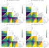 |
Fig. 3. Scatter plot between all possible free parameter pairs, color-coded by the fraction of times (FN) a given pair of parameters has a reliability greater than 70% over the total number of possible configurations, along with the distribution of each parameter. Red points (cyan points) indicate the combination of parameters where COSTA detected a real (spurious) stream in ten random extractions of the giant+dwarf. |
The latter quantity is expected to be higher for the combinations of parameters that have a lower chance of producing spurious detection for any other choice of the other parameters, and, as such, it represents a quality flag for a given configuration. Indeed, when a parameter configuration with a low FN finds a stream, the chance that this is a spurious one is higher. In the following, we use the high-FN regions in the parameter space to label the detection as higher quality (see also below), as they represent the regions where all parameters show high reliability.
In Fig. 3, the regions of the parameter space that reach the maximum level of reliability (> 70% for all possible parameter configurations) are shown in yellow, while the quality of the configuration degrades toward the blue as the fraction of > 70% reliability decreases over the total combination including that particular pair. For the yellow area, this means that, having fixed two of the four free parameters, the reliability threshold is reached regardless of the values of the other two.
Looking at the results for the different Npart − Δv cases, we can see that regions with FN ∼ 1 are located in the upper-right corner of the k − n panel, on the diagonal of the k − Nmin projection, at the bottom right corner of the k − σcut, n − σcut and of the Nmin − σcut panels, in the upper-left corner and right side of the n − Nmin projection. This is valid for all Npart − Δv, but with different extensions. Moreover, many other regions in the parameter space have an FN > 70% (light green color), indicating that there are numerous highly reliable combinations of the four parameters, which hence produce very reliable streams with little or no chance of being spurious. The same figure also shows the 1D distribution of all four COSTA parameters, corresponding to Rel > 70%, highlighting the peak values in the parameter space that allow the greatest chance of producing little or no spurious streams.
In particular, the distribution of Nmin shows that this is a critical parameter to avoid spurious detections, as the probability of finding spurious structures (i.e., groups of particles with similar velocities) is larger for small Nmin and monotonically decreases as Nmin increases, producing a higher overall reliability at larger Nmin. Indeed, too-small Nmin would increase the chance of a group of particles in k neighbors having close velocities, thus returning a spurious detection. On the other hand, as Nmin defines the minimal mass of the stream that COSTA would detect, too large an Nmin will produce high reliability but also high incompleteness in the final list of stream candidates (as small streams would be filtered out).
The distribution of σcut, instead, justifies our choice to employ many cut-offs, as larger values allow us to find warmer streams with larger Nmin (FN is close to 1 in the bottom right of the Nmin − σcut panel), while lower σcut minimizes the number of spurious structures (from the 1D distribution of the σcut fraction). Concerning the σcut parameter, it is worth mentioning that in some cases we adopted cut-offs lower than the nominal instrumental errors. This is because a stream with an intrinsic velocity dispersion smaller than the instrumental error would give an observed value that can be any random number lower than Δv. Hence, using σcut ≥ Δv would exclude any real stream colder than Δv. Using smaller cuts, we expect to detect such streams, although we cannot evaluate their intrinsic kinematics. In these cases, we consider the σmea ∼ σobs, that is, without subtracting Δv in quadrature, and we mark the latter with an apex.
Looking at the n distribution, the setups with the highest reliability fractions are located at high n, since a shallow sigma clipping removes fewer outliers. Hence, only structures with an initial low-velocity-dispersion value fall below a given threshold, unless one sets a higher Nmin, in which case there is little chance of finding a spurious structure with small n (see e.g., the central panel in the top left of Fig. 3).
Finally, the k distribution increases monotonically. Since the higher k is, the larger the possible values of Nmin (Nmin is varied from 5 up to k) are, it is expected that this distribution mimics the trend of the Nmin one.
As all the previous considerations may be dataset dependent, it is crucial to explore the behavior of the reliability in the parameter space as a function of the number of particles, the velocity errors, and also the minimal reliability threshold (e.g., changing this to a lower or higher threshold than 70%). In this section, we consider the first two quantities (number of particles and the velocity errors), while we discuss the reliability threshold in Sect. 3.6.
By comparing the top-right panel of Fig. 3, which shows the case of a lower Δv = 10 km s−1 with the top-left panel, which shows Δv = 40 km s−1, the number of possible combinations that have Rel ≥ 70% increases by more than 10% when considering smaller errors. In fact, the smaller velocity error values allow COSTA to more efficiently recognize the absence of streams without spurious detections. This is quite encouraging, as it shows that there is little room for spurious cold structures to be produced by the white noise of the background velocity field. Also, this shows that the velocity measurements are crucial to increasing the purity of stream detection.
The bottom-left and bottom-right panels of Fig. 3 show the configurations with 1000 and 500 particles with Δv = 40 km s−1 and Δv = 20 km s−1, respectively. These situations exhibit a wider parameter space with high FN (i.e. high reliable setups), similarly to the case of 2000 particles and Δv = 10 km s−1. This is likely because the smaller number of particles further reduces the effect of the noise for a given Δv, and consequently the probability of COSTA finding a spurious structure becomes lower. However, the smaller number of particles also decreases the sampling of the stream and its signal, overall decreasing the signal-to-noise ratio by roughly  . The consequence here is that COSTA might not detect the stream with the same efficiency as it would for higher numbers of particles. Thus, it is essential to also test the detection ability of COSTA as a function of Npart when a stream is present in the detection sample.
3.4.2. Stream detection
We then ran COSTA using all setup configurations with Rel ≥ 70% over the DS made of the gE0 and dwarf/stream particles, to test the algorithm’s ability to detect cold structures embedded in the hot environment of the central galaxy. We repeated this procedure ten times in order to take into account statistical fluctuations due to a random extraction of the detection sample particles. Furthermore, in order to reproduce a lower limit for the surface brightness of the extracted stream, we imposed a minimum number of ten particles to be picked up in an area of about 40 kpc located in the tail of the dwarf. These numbers correspond to a stream with a surface brightness of the order of 28−30 mag arcsec2 (see discussion in Sect. 4.3)2.
We note that COSTA does not only detect streams in the proximity of the dwarf, but it also correctly identifies other groups of stream particles, including portions of the stream that are far from the dwarf body. However, these latter detections are fairly occasional because particles that are far from the dwarf have spent more time in the halo of the host galaxies and have started to mix in the phase space of the host halos to be detected as part of a decoupled stream (see discussion in Sect. 3.4.4). It is likely that streams detected from COSTA contain, along with the actual dwarf particles, also some contaminants, meaning particles close to the stream that accidentally also have similar velocities to those of the dwarf’s particles. This “contamination” is a critical parameter to evaluate because contaminants alter the inferred stream properties. Since we know from the simulation which of the systems the particles belong to, we used this information to estimate the contamination fraction (see Sect. 3.4.3). Regardless of the mix of the dwarf/stream particles with the background main galaxy particles, we expect that the stream particles closer to the dwarf body are the ones that most keep their kinematics clearly decoupled by the hot background (see also Sect. 3.4.4). Among all candidate streams that COSTA recognizes on the DS, we consider the ones where COSTA correctly identifies at least four particles of the stream/dwarf, or where at least one third of the total particles (dwarf + contaminants from the main galaxy) is from the stream/dwarf, as true detections.
The final results of COSTA true positive detections are shown also in Fig. 3. Here, we overplot the combination of parameters where COSTA found the stream (i.e., true positives, red points) and spurious groups (i.e., false positives, cyan points), in the ten repeated DS extractions, on the density plots in Fig. 3. In many panels, real (red points) and spurious (cyan) streams are clustered in different regions, even though it is not always simple to see this. The most evident case is the Nmin − σcut plot, where red points are slightly shifted toward the right corner, where FN is higher. More quantitatively, in the Nmin − σcut projection of the case with 2000 particles and Δv = 40 km s−1, the median FN for true positive equals 0.88, while that of spurious streams is only 0.73.
Another useful projection that slightly separates real streams from spurious ones is the n − Nmin in the middle of each corner plot. This panel shows the compromise between how strong the sigma clipping can be depending on the minimal number of particles expected in the stream. Indeed, a closer inspection of the n − Nmin plot reveals that many spurious structures have been detected in the bottom-left region, while red points tend to cluster in the upper right. Being more quantitative, the median FN of red and cyan points in the n − Nmin panel are 0.58 and 0.49, respectively.
Thus, in order to minimize the chance of over-collecting spurious streams, we adopted a threshold on the FN in the n − Nmin panel. In particular, setting a minimum value of FN = 0.5, we removed about 50% of the spurious structures. We note that, despite the separation being clearer in the σcut − Nmin panel, we prefer to set a threshold in a perpendicular direction of the parameter space, with respect to σcut, in order to reduce the chances of biasing the final selection in a projection that is strictly related to a stream’s physical properties. In fact, a further clean involving σcut might alter the estimated stream kinematics. Since some of the very low FN regions lie at high σcut values, removing such regions would rule out all the combination of parameters with σcut close to the actual dwarf velocity dispersion (77 km s−1, see also Table 1).
In the following, we use this threshold as a further condition on the detected structures to clean out our list of candidate streams. The effectiveness of this choice becomes clearer in Sect. 3.4.4.
In Table 2, we report the fractions of setups that reveal the stream tail without any false positive (called f hereafter), averaged over ten simulations returning at least one detection (i.e., either a true or false positive), with and without applying the threshold of FN = 0.5. We also report the contaminant fraction, which is defined in Sect. 3.4.3.
Adopted configuration (Col. 1); fraction of setups where the stream has been recovered with respect to the total setups in which COSTA detected at least a cold substructure averaged on ten simulations (Col. 2); the contaminant fraction (CF: see definition in the text) (Col. 3).
Generally, the threshold in n − Nmin increases the number of setups where the stream is recovered. This is particularly evident for the best case with Npart = 2000 and Δv = 10 km s−1, where the fraction of setups returning streams with no spurious is ∼67% when applying the threshold of FN = 0.5 in the n − Nmin plane, while it is ∼54% withouth any threshold in FN. Given the uncertainties, however, this makes very little difference. The same can be said for the impact of changing the number of particles and adopting different velocity uncertainties. Going from 2000 to 1000, keeping Δv fixed to 40 km s−1, f goes down from 0.54 to 0.40, but it is always consistent within one-σ errors.
Lower velocity errors tend to shift detected streams toward “more reliable” regions of the parameter space. This is also visible directly from Fig. 3, comparing the top-left and top-right panels and again using the n − Nmin – and the Nmin − σcut panels to discriminate between real streams and spurious ones. Yellow regions are more extended in all panels for Δv = 10 km s−1.
The bottom-left panel of Fig. 3 shows the results of the case of 1000−75 giant-dwarf particles and Δv = 40 km s−1. Here, COSTA is still able to detect the stream, even though the ratio of the number of setups where the stream was recovered over the total number of setups is the lowest (see Col. 2 of Table 2), with and without the threshold.
Finally, we consider the case with 500−38 giant-dwarf particles. Here, we show the result for Δv = 20 km s−1 in the bottom-right plot of the same figure. This is in fact the precision one can obtain with typical mid-resolution spectroscopy. In this case, COSTA is also well able to catch the stream in a quite ample range of configurations in the parameter space (∼50%).
In conclusion, for all the different configurations we tested, when changing the number of particles and the velocity accuracy, COSTA is able to recover the stream in a relatively broad space of parameters (ranging between 40% and 67%). We note that a 50% success rate is acceptable in blind stream searches if one wants to find a list of candidates to follow up on, and if they represent a fair compromise between purity (no false positives) and completeness (i.e., find as many real streams as possible; see also Sect. 3.4.3).
3.4.3. Completeness and contamination
We can now better describe and quantify the stream properties as returned by the different setups. So far, we have identified the setups that give the true positives, but every setup produces different groups of particles, including real stream particles. In particular, we can check the degree of contamination introduced by the different setups with the aim of finding a method to define the best setup (e.g., the one optimizing the ratio between the number of real particles and contaminators). To do that, we defined the observed completeness (OC) as
This parameter is clearly complementary to the contaminant fraction (CF) of the stream (i.e., CF = 1 – OC):
The mean CF derived over all of the setups producing no false positive (Col. 3 of Table 2) are always ∼65−70%, almost independently of the sample size and velocity accuracy, which, by definition correspond to ∼35−30% of OC. This high fraction of contaminants can significantly affect the conclusion about physical properties of the stream (see e.g., Sect. 3.4.4). However, we stress that these quantities are an average over many setups, and, in principle, one can define the optimal setup that maximizes the OC. We consider this optimization in more detail in Sect. 4.5. We also remark here that the contaminant fraction does not impact the detection of the stream that remains a good candidate for subsequent follow ups. These are needed in any case to obtain the physical properties of the stream (luminosity, colors, surface brightness, kinematics, etc.).
3.4.4. Stream kinematics
After having demonstrated that COSTA is able to detect a stream, we are interested in extracting physical properties from the recovered stream. In particular, we are interested in deriving kinematical information concerning the stream from the velocities of the tracers collected as part of it. Hence, we want to find a rule of thumb to apply to the many configurations that find the stream and identify the setups that better characterize its kinematical properties (e.g., its velocity dispersion).
Sadly, a dynamical definition of the stream velocity dispersion is not straightforward, even in simulated samples like GalMer. Technically, the stream is made of all the particles left behind by the disrupting dwarf, which have a different degree of mixing depending on the time at which they became unbound. In Fig. 4, we compare the position and velocity distribution of particles belonging to the galaxy background (in gray), the ones belonging to the outskirts of the dwarf galaxy (in yellow, of which the center is shown as a red cross), and the stream particles (in blue) for one of the runs discussed in Sect. 3.4 and two different Nmin values (Nmin = 15 top, Nmin = 30 bottom). In the same figure, we also plot the true stream particles detected by COSTA in this run (in green), and contaminants that COSTA selected but are instead not part of the true streams (in red). From this figure, we can see that the stream particles (blue) overall have a wider distribution with respect to both the dwarf body particles (yellow) and the ones that COSTA detects in the proximity of the dwarf (red and green), while they are not as dispersed as the gray particles of the central galaxy halo. As such, they are both unbound from the parent dwarf and unmixed with the host halo, hence their velocity dispersion does not have a dynamical meaning because hydrostatic equilibrium does not hold. On the other hand, the “youngest” regions of the stream (green particles) show a distribution that is similar to the ones of the dwarf particles (yellow) at the equilibrium. Thus, the particles recently lost in the tail (and more likely detected with COSTA) keep the record of the kinematics of the parent galaxy3. This means that these latter particles have not yet fully dynamically decoupled from their progenitor, and we are motivated to compare their velocity dispersion with the dwarf velocity dispersion (i.e., 77 km s−1; see Table 1). This is useful for two main reasons: (1) algorithm-wise, this is the best way to identify setups that better describe (dynamically motivated) kinematical properties of a detected stream; and (2) dynamically, we postulate that the stream velocity dispersion should follow the Faber-Jackson relation (Faber & Jackson 1976) of the parent dwarfs (i.e., the velocity dispersion should correlate with the luminosity of the progenitor, if any). To illustrate how this works via data, looking at Fig. 4 again we clearly see a typical situation of a stream detection where stream particles (including some contaminants) are close to the bulk of the parent galaxy.
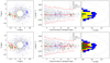 |
Fig. 4. Top: relative positions (left panel) and reduced phase space (right panel) in the case of the stream recovered with Nmin = 15. Bottom: same as above but with the stream recovered with Nmin = 30. Light gray points are gE0 particles, while blue ones are those belonging to the dE0. Yellow points represent dwarf particles within three effective radii from the dwarf center, while the recovered stream is colored in green (real stream particles) and in red (contaminants). Blue crosses indicate a group of particles further away from the dwarf main body, detected by COSTA in some runs (see text for details). |
For both the case with Nmin = 15 and that with Nmin = 30, COSTA selects only a limited fraction of particles, and it selects them very close to the dwarf (tail). The ratio of the red particles over all particles (i.e. red + green colors in Fig. 4) gives the OC, which decreases toward higher Nmin (e.g., 0.56 vs. 0.40). On the contrary, the overall velocity dispersion increases from the Nmin = 15 to 30 (as seen in both the phase-space diagram, the velocity-radius plot in the middle panels, and the velocity histogram in the right panels), and, in the latter case, it becomes closer to the one of the dwarf (i.e., 77 km s−1). Green and red particles have rather similar velocity dispersion values both in the case with Nmin = 15 (top row in the figure): σgreen, 15 = 40 km s−1, σred, 15 = 35 km s−1, and the case with Nmin = 30 (bottom row in the figure): σgreen, 30 = 74 km s−1, σred, 30 = 83 km s−1. This suggests that the contaminants only slightly alter the true velocity dispersion of the stream.
Only in very few runs does COSTA also detect groups of particles in the tail of the stream that are further away from the dwarf main body, on the opposite side of the central galaxy (see e.g., blue crosses in Fig. 4). This shows that COSTA can, in principle, also identify portions of the debris of a stream in absence of a close dwarf (e.g., at the pericenter/apocenter of stream orbits where lost particles tend to accumulate around zero systemic velocity in the reference frame of the central galaxy). This is due to the fact that, being stream (blue) particles still unmixed with the halo, they are also recognized as cold substructures.
The fact that the majority of the detections occur in the regions close to the galaxy depends strongly on the fact that these particles are fully unmixed. For a detection to occur at greater distances, one needs an ad-hoc combination of poor mixing and occasional overdensity, which is more unusual. It remains that the velocity dispersion of these latter detections cannot be dynamically connected to the parent dwarf (e.g., via a Faber-Jackson relation). The only case in which one is motivated to dynamically interpret the velocity dispersion of an isolated group of particles that has no clear dwarf association is in the one with evidence that the parent dwarf has recently been disrupted and the remaining particles are the latest lost.
Finally, since we postulate a connection between the kinematics of the stream and the one of the parent dwarf (e.g., a sort of Faber-Jackson stream), and given that COSTA can detect the same stream with different configurations, we wish to check whether we can identify configurations that reproduce, as close as possible, the real internal dispersion of the dwarf. In Fig. 5, we show the density plot of the velocity dispersion estimates of the selected stream particles as a function of the most sensitive parameter discussed in this paragraph, Nmin. In particular, we show the values obtained using a threshold on FN = 0.5 in the n − Nmin space as described in Sect. 3.4.2.
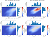 |
Fig. 5. Density plot of number of setups with a reliability above the selected threshold and with FN (≥0.5) in the n − Nmin space. Data were smoothed with a Gaussian kernel with a bandwidth equal to three bins. |
The four plots correspond to the measured velocity dispersion, σmea, from the streams selected according to the four different cases as in Fig. 3. Overall, we notice that the velocity dispersion estimates tend to cluster around the true value of the dwarf (77 km s−1), with the tails toward lower values. This happens regardless of the sample size and velocity errors, although higher velocity accuracy (e.g., Δv ≤ 10 km s−1, top right panel, and Δv ≤ 20 km s−1, bottom left panel) gives less pronounced tails toward low σmea in the velocity distribution. This is particularly evident when comparing the 2000-particle cases (top row of Fig. 5).
Being more quantitative and using the median of the distribution as a probe of the peak, we obtain the following stream velocity dispersions: 43 ± 23 km s−1, 57 ± 12 km s−1, 57 ± 15 km s−1, and 57 ± 18 km s−1 for the 2000 (40), 2000 (10), 1000 (40), and 500 (20) cases, respectively.
Of course, the final dispersion of the stream is in all cases affected by the contaminants from the main galaxy, but overall the median values are always consistent within 1-σ uncertainties and are all close, although slightly lower, to the true velocity dispersion of the dwarf. This implies that the contaminants selected by COSTA as part of the stream are almost statistically indistinguishable from the stream particles, as they hold similar overall kinematics (see Fig. 4).
3.5. The case of the gSa-dS0 encounter: Testing COSTA on a cold system
Having demonstrated that COSTA is able to find cold streams embedded in the halo of hot early-type systems, we now need to test the case of late-type galaxies. We selected a gSa-dS0 encounter, and tested both a prograde and a retrograde motion for the dwarf, because the stronger rotation of the galaxy disk might have a different impact in the two cases. We followed the same steps as in the gE0-dE0 case, and we highlight the results in the following sections.
3.5.1. Reliability
First, we ran COSTA over the WNS using all parameter combinations to determine the reliability distribution in the parameter space. In Fig. 6, we show the reliability maps for the prograde and retrograde cases on two separate rows. Also in this case, we show the density plot obtained with different numbers of particles for the giant and the dwarf and different values of Δv.
Since the gSa is colder than the gE0, it is much easier for COSTA to find combinations of galaxy particles with a local velocity dispersion close to that of the σcut (i.e., there is a smaller contrast). It is much easier for COSTA to find spurious substructures, and consequently it is harder to find setups with high reliabilities (i.e., with more than 70% of detections being non-spurious). As a result, the regions of the parameter space with high FN (yellow) are considerably reduced with respect to the gE0 case, and there is generally a higher chance of finding some false positives. As for gE0, the adoption of smaller velocity errors produces a slightly higher number of good setups, especially in the retrograde case, and the FN also increases over a relatively wider area for the smallest number of tracers tested in our simulations (fourth panel). The results for the prograde (top) and retrograde (bottom) cases are very similar because in the two cases the WNS does not change dynamically in a significant way, despite the fact that the different interaction with the intruder might have introduced different perturbations.
3.5.2. Stream detection
The second step is to run COSTA on the DS, which is made by the main galaxy and dwarf particles, to recover the stream particles. As with the gE0+dE0 encounter, we performed ten random extractions of the giant+dwarf system, imposing a limit on the lower surface brightness of the stream. The results of this test are listed in Table 3, both for the prograde and the retrogade encounters. In general, COSTA only detects the stream in few setups (with reliability Rel ≥ 70% ≥ 70% both for the prograde and retrograde motions). Furthermore, in the gSa-dSO case, most of the setups that correctly found the stream particles also detected spurious substructures (see bottom-left panel of Fig. 6 or Table 3).
Overall, for the retrograde encounter, COSTA performs better, with a much lower CF (e.g., ∼15% versus ∼60% for the 2000 particles case with Δv = 40 km s−1). The number of setups in which COSTA detects a stream is also higher in the retrograde case, at least for the best possible configuration, that is, 2000 parts – 10 km s−1 (11% for the prograde and 29% for the retrograde, assuming a threshold of 50% in the n − Nmin panel, although with a large uncertainty). In this configuration, and partially also in that with 2000 particles and a larger velocity error, the stream has been detected in regions that tend to accumulate toward the highly reliable FN (yellow areas) regions in the parameter space. This is especially visible in the Nmin − σcut plot, as we see for the gE0 system. In particular, high-reliability configurations favor a smaller σcut (≤40 km s−1). However, this is not always true for the prograde and retrograde cases with a smaller number of particles, at least not for all the projections. In these cases, the stream was detected only a few times, and they are very sparse in the region of the single plots of the parameter pairs.
Finally, as seen in Fig. 6 (at least for the retrograde case), COSTA performs generally better when the velocity errors are smaller. Here, the algorithm reveals the stream in more setups.
An interesting contrast between the gE0-dE0 and gSa-dS0 cases is that, for the latter, the number of particles produces a very different number of setups with high reliability. This is valid both for the prograde and for the retrograde case. Going from 2000 particles to 500, the f is between three and five times smaller, while the CF increases.
We also note that, for the gSa-dS0 cases, and in particular for the prograde encounters, the configurations for which we correctly detect the streams are often embedded in low-FN areas. This is different from what happens in the gE0-dE0 interaction and it is due to the fact that, since COSTA finds more spurious stream, the configurations that allow us to find the stream also find some of them that are spurious, at least with the change of other parameters. This means that, even if the stream is found, this has a generally lower reliability in cold systems. We need to stress here that this conclusion is not general, as this applies to the case of a mass ratio 10:1, that is, with a small contrast between the dispersion of the stream and the dispersion of the background velocity field (see below).
3.5.3. Stream kinematics
The σcut (≤40 km s−1) is an upper limit, beyond which COSTA no longer detects the stream. The median of the velocity dispersion, using only setups with FN > 0.5 in the n − Nmin plot in the retrograde encounter, gives a velocity dispersion lower than the one of the parent dwarf galaxy (σdwarf = 74 km s−1). In fact, we obtain the following medians of the velocity dispersion distributions: 24 ± 13 km s−1, 31 ± 7 km s−1, 33 ± 2 km s−1, and 37 ± 6 km s−1 for the 2000(40), 2000(10), 1000(40), and 500(20) cases.
Here, the worse performance of COSTA with respect to the gE0-dE0 is due to little contrast between the dwarf velocity field (which is rather hot in the specific GalMer simulation; i.e., σdwarf ∼ 74 km s−1) and the gSa (σgiant ∼ 81 km s−1). Thus, the exercise we carried out here has to be interpreted as an “extreme case” to set a guideline for the methodology to follow in “real” cases, where the difference between the velocity dispersion of the dwarf and that of the giant is larger.
3.6. The dependence of COSTA’s performance on the reliability threshold
In this section, we explore how different reliability thresholds can affect the completeness and purity of COSTA. Overall, logically, a lower threshold allows us to increase the probability of finding a stream (at the expense of a greater contamination), while a higher limit has the opposite effect.
In the case of the gE0-dE0 interaction, we increased the lower limit of the reliability and we only used combinations of free parameters above 90%. We only ran COSTA on the Ngiant = 2000, Ndwarf = 150, and Δv = 40 km s−1 configurations. Of course, the number of parameter combinations overcoming the threshold is reduced with respect to the previously used threshold of 90%. This can be seen in the left panel of Fig. 7 (left panel). However, the stream is still detected in many setups, and they show almost the same distribution in the parameter space as for the lower threshold.
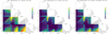 |
Fig. 7. Parameter space overlapped with true and false streams detected by COSTA for both early- and late-type galaxies, in the standard configurations (2000 particles and Δv = 40 km s−1) for three cases (gE0, gSa prograde, and gSa retrograde), but using different reliability thresholds. |
For the gSa-dSa interaction, the situation is reversed, as we lowered the acceptable value of reliability to 50%. Indeed, in both the prograde and retrograde encounters, COSTA could not find streams using a higher threshold, so we checked a lower one. In both encounters we used Ngiant = 2000, Ndwarf = 150, and Δv = 40 km s−1. In the prograde case (central panel of Fig. 7), COSTA finds the stream in a slightly higher number of setups, with respect to the very few that have a reliability cut-off of 70%. In the retrograde case (right panel of the same figure), the improvement is even higher as the number of setups where COSTA detects the stream increases by 50% with respect to the previous case. Thus, we conclude that for the late-type case, the 70% reliability threshold is too conservative, and a lower reliability threshold would give more opportunities to identify streams.
4. The case of the Fornax cluster core
We tested COSTA on a cluster environment where streams are produced in a more complex situation with many large coexisting galaxies. In such environments, multiple low-surface-brightness streams from a larger population of dwarf galaxies and with a given luminosity function and different kinematics can be produced. In particular, we present here the case of the Fornax cluster, for which there are GCs (from P+18) and PNe (from S+18) available for stream search, which we will present in forthcoming analyses. The aim of this section is to show that for a more complex case, such as the Fornax cluster core, COSTA can also be set to detect cold streams of small numbers of particles, as was done for the GalMer simulations.
For the Fornax cluster, unfortunately, we do not possess a simulation realistic enough to produce an equally large structure distribution of particles as the one reported in GC and PNe studies. We thus decided to build up Monte Carlo realizations of the kinematical tracer distribution in the 3D phase space (i.e., 2D positions and radial velocity) over which we we were able to obtain a reliability map for COSTA and test its stream detection performances.
Indeed, following the approach adopted for the GalMer simulations, we first require the Monte Carlo realizations of the Fornax core in order to have a smooth cluster background with no streams (i.e., the WNS). This allows us to explore the parameter space and assess the reliability function of COSTA as a function of the different parameters. Secondly, we added a number of artificial streams (hence generating different DSs) and ran COSTA to recover them and to calculate the OC and CF.
4.1. Monte Carlo simulations of the Fornax cluster core
To produce COSTA reliability maps, we performed a suite of Monte Carlo simulations resembling the Fornax core as closely as possible in terms of spatial distribution, local density, and radial velocity distribution of the kinematical tracers (WNS).
We only simulated the region covered by the current discrete tracer surveys (FVSS, P+18, and S+18), covering about 1.8 deg2 around the cD, NGC 1399. In this area, there are two other bright early-type galaxies: NGC 1404, located just below the cD in the south-east direction at about 9 arcmin; and NGC 1387, at a distance of ∼19 arcmin to the west of NGC 1399. A third relatively massive galaxy, NGC 1379, located at ∼60′ toward W, was observed with one FORS2 pointing in S+18. However, this system is excluded from this analysis because we do not have continuity with the rest of the Fornax core area, hence it is useless with regard to stream finding.
We generated simulated GCs and PNe in a total number that is as close as possible to what has been observed in S18 and P18. In the following, we assume that both GCs and PNe trace the same underlying population of old stars4, at the equilibrium in the gravitational potential of these three galaxies, assumed to be the superposition of the individual galaxy potentials with spherical symmetry. Following Napolitano et al. (2001), we produced the 3D position starting from a 3D spherical density profile and projected them on the 2D sky plane (X − Y in our case). For each particle, we determined the 3D velocity vector according to the hydrostatic equilibrium equations (see below), which we projected along the line of sight to derive the intrinsic radial velocity. We finally simulated a radial velocity measurement by randomly extracting the measured velocity from a Gaussian having the intrinsic radial velocity as mean and standard deviation equal to the measurement errors.
In order to produce these Monte Carlo realizations of particles sampling the total potential in the Fornax core, we assumed a total mass of about 1014 M⊙ and a Hernquist (Hernquist 1990) density distribution of the stellar-like tracers for the cluster. This is a good approximation for elliptical galaxies following a de Vaucouleurs law (1948). For NGC 1399, which gathers most of the light in the cluster core, Iodice et al. (2016) found a Sersic index n = 4.5, which is very close to the n = 4 that describes the de Vaucouleurs law.
The luminous mass density is expressed by the formula
 (3)
(3)
where Ml is the total luminous mass, a is a distance scale (Re = 1.81534 a) and C is a normalization constant. We made the same assumption for all other galaxies in the area, with the adopted parameters as in Table 4.
Parameters of the simulated galaxies.
In addition to the stellar mass density, we also considered a dark halo following a Navarro-Frenk-White (NFW, Navarro et al. 1997) profile, to define realistic internal kinematics for the simulated particles. Hence, the potential of the system at equilibrium is provided by the total mass:
 (4)
(4)
We assumed non-rotation5 and an isotropic velocity dispersion tensor, and we solved the radial Jeans equation,
 (5)
(5)
to derive the 3D velocity dispersion σ2 in the three directions of the velocity space, and we generated a full 3D phase space.
As briefly anticipated above, we simulated an observed phase space by projecting the tracer distribution on the sky plane, and we derived the LOS velocity of the individual particles. In particular, we used the X − Y plane as the sky plane and the z-axis as the LOS. However, due to the full spherical symmetry of the model, the particular projection is irrelevant.
Finally, in order to simulate a velocity measurement, we used the same approach as for the GalMer simulations: we adopted a Gaussian error distribution and re-sampled the radial velocities produced by the Monte Carlo simulations with a Δv = 37 km s−1, which is consistent with typical measurement errors from P+18 and S+18. In this case, we do not vary the errors, as this test is meant to demonstrate that COSTA can be applied to a real dataset and provide a series of reliable setups for finding stream candidates from real datasets. We will do the same in the second paper of this series.
We included 1985 particles in the simulation to reproduce the number of observed PNe and GCs selected in the area as accurately as possible. The number of points for each satellite galaxy was then obtained with a cross-match with the real data, counting the number of plausible PNe and GCs bound to the galaxies, while both effective radii and velocity dispersions are taken from the literature (see Table 4). To obtain a realistic reproduction of the PN and GC systems around NGC 1404 (in terms of number and radial abundance), we need to adopt an effective radius (i.e., the radius enclosing half of the total light of the galaxy), Re ∼ 100″, slightly larger than the one estimated by Corwin et al. (1985) (Re ∼ 80″).
For NGC 1387, we took into account the velocity offset of PNe reported by S+18 (i.e., a mean velocity higher than the systemic velocity of the galaxy reported in literature by ∼100 km s−1). Indeed in this area, we have a larger number of PNe than GCs, respectively 117 (88%) and 16 (12%), within three effective radii from NGC 1387; thus the offset of the PN velocities might generate an overall velocity excess of 100 km s−1, that we thus artificially added to all simulated points around NGC 1387 in order to match the real objects (see also Table 4).
The final result of all these fine-tuning calibrations for the simulated sample gives the distribution of the simulated particle, as shown in Fig. 8. Here, we plot the simulated points for one of the mock realizations using positions computed with respect to the simulated cluster center. We observe a fair spatial correspondence between the main galaxies in the field of view (whose positions are highlighted as black squares) and the simulated particles (red points).
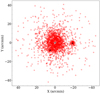 |
Fig. 8. Simulated data points for one Monte Carlo realization, with NGC 1399 at the origin of coordinates. NGC 1404 is just below the cD (X ∼ −5, Y ∼ −5), and NGC 1387 is at X ∼ −20 arcmin. The positions of the three galaxies are indicated by black squares. |
In Fig. 9, we show the phase-space distribution of the same simulated particles together with the ±3σp profiles (where σp is obtained as in Eq. (1)) of the GCs from P+18 and the PNe from S+18 (curves are extracted from Fig. 9 in P+18). Once again, the similarities are quite evident between the overall kinematics of the simulated particles and of the observed ones. Once we had optimized the Monte Carlo simulation setups to best reproduce the observed GC+PN dataset, we finally produced 100 realizations of the system, which represent the WNS from which we obtained the reliability maps for COSTA.
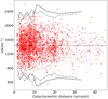 |
Fig. 9. Phase space of one Monte Carlo simulation. On the x-axis, we plot the distance from NGC 1399 in arcminutes, and on the y-axis we plot the velocities of the points in km s−1. The continuous solid and dashed-dotted lines represent the ±3σp profiles of the GCs and PNe, respectively, extracted from P+18 (their Fig. 9). The dashed black horizontal line represents the systemic velocity of NGC 1399 (1425 km s−1). |
Differently from the GalMer simulations, where the statistical variation of the parameters were obtained only by perturbing the velocities of the particles, for the Fornax-like case we re-sampled the full parameter space. Hence, we added more statistical noise to the simulated sample, coming from different spatial configurations of the same physical streams.
4.2. COSTA setup and reliability map
To obtain the reliability map, we followed the same steps as in the GalMer simulations (Sects. 3.4 and 3.5). To begin with, we ran COSTA for each parameter combination over the 100 Monte Carlo realizations of the WNS and counted the number of configurations for which COSTA finds no spurious streams.
In this case, we uniformly sampled the k, n, Nmin parameters’ space for a different σcut and ran COSTA with all the possible combinations of the free parameters selected in the following ranges:
-
k: from 10 to 50 with steps of 5.
-
n: from 1.3 to 3 with steps of 0.2−0.3.
-
Nmin: all values from 5 up to k.
-
σcut: from 10 to 120 km s−1 with steps of 5 km s−1.
The difference with respect to the gE0-dE0 case (i.e., the case of another hot systems) is the adoption of a larger σcut, k, and a larger Nmin range. This is motivated by the fact that, as the Fornax environment is hotter than the GalMer gE0, we can detect higher velocity substructures (if any). Similarly to the GalMer simulations, we also used σcut values below the instrumental errors, considering in these cases σmea ∼ σobs (see discussion in Sect. 3.4).
Figure 10 shows the reliability map, color-coded by the fraction of the number of setups with a reliability ≥70%. The case of the Fornax-like system is fairly different with respect to the configurations tested with the GalMer simulation. Indeed, the intrinsically higher velocity dispersion provides a much smaller chance of obtaining a correlated group of particles characterized by a small dispersion; this is due to statistical fluctuation in the parameter space. For this reason, COSTA has a quite large range of parameters that find a spurious stream in less than 30% of the extractions. One may argue that in this case 70% is a too-loose threshold, and higher values might be used too. However, the Monte Carlo simulations only partially catch the full statistical fluctuations, and they might be too smooth with respect to the real data. In a second step, we ran COSTA on the DS where the artificial streams were added to assess the effectiveness of COSTA detection.
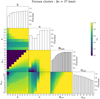 |
Fig. 10. Reliability map for Fornax cluster obtained with a reliability threshold of 70%. |
4.3. Recovering simulated substructures
When applying COSTA to real cases, detection is the minimum we want to achieve (completeness), while we can compromise on the full recovery of stream particles vs. contaminants (purity), as we correctly expected that we would lose some particles and also obtain some contaminants (non-stream particle) as part of a correctly detected stream (see also discussions in Sects. 3.4 and 3.5).
To check COSTA’s ability to recover known streams in the Fornax-like environment and to assess completeness and purity, we added three artificial streams to our Monte Carlo simulations. Since we cannot reproduce the full dynamics of a stream in our Monte Carlo simulations, and we wanted to test COSTA in more observational situations, we chose typical stream sizes and kinematics that can be realistically found in real data. As shown in the case of the GalMer simulations (see e.g., Fig. 4), despite the fact that a dwarf galaxy spreads a large number of particles along its encounter orbit, COSTA can identify only the closer ones, which were the last to be stripped (of the order of a few tens, depending on the surface brightness of a stream), spread over ∼5−15 kpc, that is, 1′−3′ at the distance of Fornax.
The first stream (stream 1, hereafter) is made of 20 particles, measures 1′ × 2′, and has an intrinsic velocity dispersion of σ = 35 km s−1. Two other streams were extracted by randomly sampling particles from the tail of the GalMer gE0-dE0 case discussed in Sect. 3.4. We isolated a group of 30 particles, distributed over an area of about 3′ × 1.5′ in one case (GalMer 1 hereafter) and 6′ × 3′ in a second case (GalMer 2), with an intrinsic velocity dispersions of σ = 45 km s−1 and σ = 62 km s−1, respectively. These two streams have the advantage of being more realistic (in shape and density) as they are based on a simulated encounter, although the dynamics of the GalMer simulation adopted is not really close to the one of the Fornax core, in particular because of the lower mass of the main galaxy as compared to NGC 1399. We also took larger streams (3′ roughly corresponds to 30 kpc) in order to explore the ability of COSTA to find larger and more diffuse streams.
The final properties of the artificial streams are summarized in Table 5.
Properties of the simulated streams.
In order to simulate a real measurement of the particle redshift, we randomly re-extracted their “measured” velocities from a Gaussian with a central velocity equal to the intrinsic radial velocity, and standard deviation of 37 km s−1. We stress here that the three streams have a velocity dispersion within the range expected for dwarf galaxies (Kourkchi et al. 2012).
Also, the number of particles is not arbitrary: indeed, assuming that we split the particles in the same number of PNe and GCs, and assuming a typical (bolometric) PN-specific number density of 50 × 10−9 PN/L⊙ (see e.g., Feldmeier et al. 2004), the luminosity in the g-band corresponding to 10−15 PN-like particles is of the order of 108 L⊙. The corresponding surface brightness of streams, with sizes as in Table 5, is of the order of 28−29 mag arcsec−2, which is close to the typical low-surface-brightness levels expected for these substructures (see e.g., Cooper et al. 2010).
At this point, we built a set of Monte Carlo simulations to which we added the particles of the three simulated streams each time randomly varying their mean velocity using a Gaussian with a 0 km s−1 mean, assuming the cD at rest in the cluster center, and with a standard deviation of 300 km s−1, which is similar to the velocity dispersion of the Fornax cluster (see P+18 and S+18 for a discussion). We also systematically randomized their positions to recover them in three different ranges of cluster-centric radii, in order to verify a dependence of the recovery rate with the distance (and hence the local particle density). We chose three shells: R = 5′−7′, R = 7′−12′, and R = 12′−18′, while we excluded the region within 5′. Here, the light is too dominated by the cD and it would be very hard to detect low-surface-brightness structures. We did not place the streams at distances larger than 18′ in order to be conservative, as in less dense regions the frequency at which the stream is recovered could be overestimated because of a lower background. Furthermore, the stream GalMer 2 was only inserted in the two external shells because this diffuse stream is typical of longer lived passages happening far from the cluster center (see e.g., the tail of the encounter in Fig. 1).
As for the GalMer systems, we ran COSTA on 10 out of 100 of the Monte Carlo simulations from the reliability run to evaluate the stream-detection performances. The results for the three streams at different radii and their reliability maps are displayed in Fig. 11 and listed in Table 6.
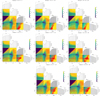 |
Fig. 11. Stream (red points) and spurious structures (cyan points) overlapped on Fornax cluster reliability maps in the different shells (left columnR = 5′−7′; middle column R = 7′−12′; right column R = 12′−18′) and for the three different simulated streams (top: stream 1, middle: GalMer 1, and bottom GalMer 2). |
The general result is that COSTA is able to recover all streams with a broad number of setup parameters. On average, recovery increases slightly for the GalMer streams at greater distances, mainly because the signal from the particles belonging to the stream is higher with respect to the noise of the hot environment (with lower local density). This does not happen for stream 1, which is smaller and more compact. Specularly, the contaminant fraction decreases with increasing radius, and this is true for all the streams.
4.4. Stream kinematics
The only aspect of the algorithm we wish to discuss in more detail at this level is how much (and what kind of) physical information COSTA can provide, besides the stream detection. In fact, despite the detection being important per se, as it provides candidates for follow-up observations (e.g., deep imaging, higher resolution spectroscopy), having predictions about relevant intrinsic properties such as surface brightness, a reliable estimate of the velocity dispersion, and, possibly, the membership of particles, is fundamental to planning such follow-up programs.
As introduced in Sect. 4.3, the estimation of the true kinematics of the stream is equivalent to estimating the real number of true particles belonging to the stream and the fraction of contaminants from the background system as a function of the setups. In principle, one may think that this should depend on the structure of the stream: compact, well-populated, and very cold streams should produce almost no contaminants, while very diffuse warmer streams would more easily be contaminated by particles of the galaxy halo, which have similar velocities to those of the central galaxy. However, as we discuss in Sect. 4.5, contaminants do not have a huge effect on the estimation of the velocity dispersion of the stream, since by construction COSTA picks up particles with similar velocities.
In Fig. 12, we show the density plot of the recovered streams in the Nmin − σ diagram, which were cleaned using a threshold of FN = 0.5 in the n − Nmin panel, only for the R = 7′−12′ shell, as indicative of the ability to recover the stream kinematics. The results for the other two annuli are similar to those obtained for the central one. We note that, differently from the GalMer simulations, we constructed the streams with a given velocity dispersion, and thus we can check if the real value is recovered. From the figure, it is evident that the setups via which the stream is detected accumulate around the true velocity dispersion of the streams (35 km s−1, 45 km s−1, and 62 km s−1 for stream 1, GalMer 1, and GalMer 2, respectively), indicated by the dashed black line. In particular, the median of the σmea distribution is found to be 16 ± 24, 52 ± 15, 62 ± 28, which is consistent within 1σ uncertainties.
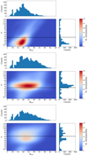 |
Fig. 12. Density plot in Nmin − σ diagram, and number counts of the recovered artificial streams for the middle shell (i.e., 7′−12′) for stream 1 (top), GalMer 1 (middle), and GalMer 2 (bottom). The horizontal dashed line shows the true velocity dispersion of each stream. The sample was cleaned by using FN = 0.5 as the threshold in the n − Nmin space. Data were smoothed using a Gaussian kernel with a bandwidth equal to 3. |
We notice that the difference between the median values and the true velocity dispersion values are of the same orders of magnitude as normal measurement errors for mid-resolution spectroscopy. For stream 1, however, the mean value is below the accuracy allowed by the velocity, hence the median value just reveals that the assumed precision does not make it possible to recover the true kinematics, for which a higher velocity accuracy is required.
We also estimated the median number of particles recovered for each stream so as to check whether COSTA allows us to infer the total “luminosity” associated with the stream, and we found a median of Nrecov = 22, 31, 29 for stream 1, GalMer 1, and GalMer 2, respectively. These median values are very similar to the true number of particles belonging to the stream (20, 30, 30; see Table 5), even if we do not expect that all of these particles truly belong to the stream (see discussion in the next session).
4.5. Contaminants and fraction of recovered particles
We evaluate here the fraction of contaminant (CF, defined in Sect. 3.4.2) particles within the different streams as a function of the different parameters. We used the Fornax simulations to decipher how the contamination can change depending on stream compactness (from the compact stream 1, to the very diffuse GalMer 2), internal velocity dispersion, and position within the central potential. We stress that this is a test that one can do only a-posteriori, by placing stream candidates in the Monte Carlo simulations at the right distance and with the right geometry to perform a “contamination run”. Nevertheless, this is useful for assessing the realistic contamination of a given stream.
Our main goal is to provide a general example of the impact contaminants have on the inference one can derive from COSTA candidates and on the intrinsic properties of the streams. We show in Fig. 13 the trend of CF as a function of the different setup parameters for every shell of the three streams. We see a clear dependence of the CF on Nmin and on k: thus, the larger Nmin and k are, the higher the number of contaminants is. This is valid for all the streams, in all the shells, but the slope of stream 1 is steeper and reaches a larger CF, especially for Nmin. A similar trend is also present for the velocity dispersion cut-off, although it is more noisy and dependent on the shell one considers (more evident at lower radii; for n, instead, the CF is constant around CF ∼0.2−0.3).
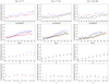 |
Fig. 13. Contaminant Fraction as a function of setup parameters for R = 5′−7′ shell (left column), R = 7′−12′ shell (middle column), and R = 12′−18′ shell (right column). Red points are for the GalMer 1 stream, green points for the GalMer 2 stream, and the blue points are for stream 1. |
In the worst cases, we see an increase up to 60% for stream 1 and ∼40% for the two GalMer streams, σcut > 100 km s−1, and Nmin > 35. The main reason for the greater contamination is that, while the number of recovered true particles remains almost constant, the larger σcut and Nmin make COSTA select more particles that have compatible velocities, but that do not belong to the stream. For k = 50, the CF reaches the highest level of 50% for the inner radial bin, while it stays below 40% for the outer ones. For any value of n, the CF is always below 40%. In this case, it is also on average lower for the outer bins with respect to the inner one.
The number of particles recovered has a strong dependence on the number of k (neighbors), as we can expect, and it also has a small dependence on the value n of the sigma clipping: higher values of n give better results. Completeness and contaminant fractions are very similar in the case of the two GalMer streams, even if they are different sizes. This suggests that COSTA is able to recover even diffuse streams; for example, the recovery frequency is independent of the dimension of the structure. However, we do speculate that it could be harder to detect these kinds of streams in the denser region, where the noise due to the hot component of the cluster increases.
It is also instructive to verify the correlation between the number of the recovered particles and the setup parameters. To do that, we define the true completeness (TC) as
where the true stream particle numbers are given in Table 5 for the three simulated streams. The TC is used here to decipher the range of parameter setups that maximize the number of recovered particles compared to the real ones, by contemporary imposing a low CF.
All quantities listed above are not known in observations and depend on the specific dataset and on the distance (i.e., the local particle density). To investigate the effect of distance, we plotted the values of the TC parameter (transparent triangles) and of the OC parameter (full dots), defined in Sect. 3.4.2, for the three simulated streams in the three different shells.
Overall, the TC tends to rise with increasing values of all the setup parameters. This indicates that COSTA recovers more particles by using stronger constraints (i.e., greater numbers of neighbors and particles). However, this also causes a higher number of contaminants, as seen in Fig. 13. We also note that the behavior of the TC is more “extreme” in the cases of the GalMer streams (red and green points). We speculate that this may be due to the fact that stream 1 is much more compact than the other two. The observed completeness (full dots) instead decreases for larger σcut, Nmin, and k while it stays roughly constant all along n values.
A compromising rule of thumb we derived when cross-checking Figs. 12–14 is that if a stream is found with different setups with similar reliability, one should first select the parameters that better reproduce its kinematics: the median of the distributions shown in Fig. 12 for Nmin and σcut. Then, one should try to select values for n and k, for which the OB and TC are similar, while the CF is the minimum possible. For the streams simulated here, this region is around the following values: k ∼ 25−30 and n ≥ 1.8. This should allow for a reasonable level of completeness (∼80%), with a contamination that is ∼50% in the worst case (i.e., high σcut), or lower than that. It is important to stress, however, that these numbers depend on the system one considers and on the morpho-kinematic characteristics of the streams one aims to recover. Thus, each run of COSTA needs to be properly trained with ad-hoc Monte Carlo simulations before the algorithm can be used with real data.
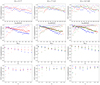 |
Fig. 14. Observed completeness (full dots) and true completeness (transparent triangles) as a function of the setup parameters for R = 5′−7′ shell (left column), R = 7′−12′ shell (middle column), and R = 12′−18′ shell (right column). The color-code is the same as in Fig. 13: red points for GalMer 1, green points for GalMer 2, and blue points for stream 1. |
Finally, we checked how accurately COSTA can reconstruct the intrinsic properties of the streams. The presence of contaminants (estimated to be of the order of 20% of the total number of particles for low σcut, if the rule of thumb holds) is expected to alter the properties of the recovered stream. In fact, these should have hotter kinematics and be characterized by a higher velocity dispersion. However, to be selected as friend-of-friend particles, they likely have velocities reasonably compatible with the bulk of the stream, so the effect should not be dramatic. From Fig. 12, we see that the smaller the cut-off, the smaller the measured stream dispersion; although, if the adopted cut-off is larger than the real stream dispersion, the dispersion estimates tend to saturate around the true dispersion value. This implies that if using a too large a cut-off does not produce a dramatic overestimate of the true velocity dispersion, too small a cut-off might produce an underestimation of the stream’s velocity dispersion. Thus, adopting a larger cut-off would be the safest choice. It would give a more realistic estimate of the stream dispersion, but, as discussed before, this is at the cost of a larger fraction of contaminants.
Overall, both the number of particles of the stream and the stream velocity dispersion are underestimated by COSTA. These two quantities are the major parameters we want to retrieve for our stream candidates, because they can give information about the amount of dispersed stellar mass per event and the dispersion of the parent dwarf galaxy (and likely its virial mass). However, the optimization of the setup in view of recovering the best estimates is beyond the current goals of the preliminary test carried out in this paper, as we are primarily interested in the detection of the streams. In conclusion, for what we have discussed in this section we are confident that COSTA is able to find real streams in our data, if any.
5. Conclusion
In this work, we introduced the COld STream finder Algorithm: a new tool used to detect cold kinematic substructures in the outer halos of massive galaxies, as a probe of their recent and past merger history. As all massive galaxies build their halos through minor mergers (e.g., Amorisco 2019), it is of great value to reveal such tidal debris and infer their intrinsic properties in order to unveil the mechanisms playing a role in the mass assembly history of massive galaxies.
Since these structures have very low surface brightnesses, it is incredibly difficult to detect them by means of photometric observations alone. In the last years, thanks to new instrumentation that allowed for more accurate spectroscopy, the research of merger signatures shifted to the exploration of the phase space of kinematical tracers. So far (supported by numerical simulations and analytical models), the detection of streams has been limited to the search for shells and narrow diagonal tracks, which have a chevron-like shape in the position-velocity diagram (e.g., Romanowsky et al. 2012; Longobardi et al. 2015). Unfortunately, these patterns are not produced by low dispersion streams made of a handful of particles (of the order of a few tens) and originated from dwarf galaxies in a recent encounter with a massive galaxy (see e.g., Fig. 4). COSTA allows us to search for these low-surface-brightness streams in the phase space in a systematic way. It also makes it possible to detect cold kinematic substructures moving in a warm/hot environment composed of relaxed particles. COSTA relies on a deep friend-of-friend algorithm that, through an iterative sigma clipping, detaches groups of neighbor particles with cold kinematics (with velocity dispersions of the order of tens of km s−1). The algorithm has four free parameters that have to be set with Montecarlo simulations, mimicking the real system under examination.
The final aim of this work has been the detection of streams with COSTA in simulated systems, and we are fully confident that our algorithm is also able to detect them in real cases. In particular, in this work, we did the following:
-
We discussed the ability of COSTA to recover cold substructures in different dynamical conditions, from cold giant spiral galaxies to giant ellipticals living in the core of large clusters of galaxies (Sects. 3 and 4). The general result is that COSTA is able to detect real substructures with a variety of combinations of the four free parameters, and with a limited number of spurious events, if one selects the regions in the parameter space that maximize the reliability of a stream detection and minimize the chance of false positive.
-
We showed that the COSTA algorithm can find cold streams embedded in a hotter environment. The efficiency of COSTA in recovery streams heavily depends on the ratio between the velocity dispersion of the stream and that of the host galaxy, favoring cold streams embedded in a hot surrounding. In fact, the performance of COSTA is much worse when the difference between the velocity dispersion of the giant and that of the dwarf intruder is very small (see the case of a gSa-dSa interaction, Sect. 3.5, versus the case of a gE0-dE0 interaction, Sect. 3.4, and that of the Fornax core, Sect. 4). The algorithm also depends somewhat on the number of tracers of the stream (i.e., the mass ratio of the dwarf and the giant galaxy; see Sect. 4).
-
We showed that the difference between the measured and the real velocity dispersion is similar to the uncertainties on velocities, hence the assessment of the stream kinematics would improve if higher spectroscopic resolution is available (section Sect. 3.4.4).
-
We demonstrated that in order to best estimate the reliability of the COSTA setups, we have first to construct a realistic realization in the phase space of the system under analysis. This is not an easy task and it also requires customized Monte Carlo realizations (Sect. 4). Furthermore, the reliability map one can derive might depend on how accurate the description of the underlying “relaxed” system is with respect to the stream population. However, we note that an over-detailed dynamical description of a given system can also incorporate substructures as a part of the relaxed component, hence reducing the chance of being recognized as a true substructure. We believe that the Monte Carlo approach, as in Sect. 4, is a reasonable start, but we cannot exclude that a more sophisticated relaxed model based on N-body codes will be used in the future to refine the predictions on real systems applying COSTA to real data.
-
We derived a rule of thumb to unveil the real kinematics of a given stream, and hence to obtain insights on the properties of the parent galaxy from which these particles were stripped. We note, however, that COSTA generally underestimates the true velocity dispersion of the stream (Sect. 5).
To conclude, we prove here that COSTA is a useful tool in detecting stream candidates that originated from close galaxy encounters in a 3D phase space. It uses the right ascension, declination, and radial velocity of particles as input. Since its ability increases when the stream is considerably colder than the surrounding environment, its natural implementation concerns galaxy clusters in which the high velocity dispersion of the relaxed particles moving in the potential well of the cluster makes it easier to unveil a group of particles coherent both in position and in velocity. Nevertheless, we demonstrate that COSTA is also suitable for other situations, such as galaxy-galaxy encounters; hence, in principle it could be used wherever a sample of kinematic tracers is available.
We stress here that this condition has been imposed regardless of the Npart, which might bias the detection toward intrinsically denser streams for lower Npart, and, as such, increase the detection power of COSTA for these cases. As we are interested in covering a variety of observational conditions, we kept this condition; however, we take into account the detection efficiency as a function of Npart when drawing conclusions.
Dynamically speaking, this means that both the energy transfer from orbital momentum to the dwarf GCs (e.g., via tidal approximation; see Napolitano et al. 2002) and the dynamical friction ( , where the density, ρ and the inverse of the velocity dispersion
  of the environment are small) have a minor impact on the stripped particles.
For a discussion about the statistical similarity between the two tracers (see Napolitano et al., in prep.).
Although some rotation of blue GCs in the radial range between 4 and 8 arcmin was measured, the kinematics of the outskirt of NGC 1399 is dominated by the random motion (Schuberth et al. 2010; Coccato et al. 2013).
Acknowledgments
NRN acknowledges financial support from the “One hundred top talent program of Sun Yat-Sen University” grant N. 71000-18841229, and from the European Union Horizon 2020 research and innovation programme under the Marie Skodowska-Curie grant agreement n. 721463 to the SUNDIAL ITN network. MG acknowledges support from the INAF fund “Funzionamento VST” (1.05.03.02.04). CS is supported by a Hintze Fellowship at the Oxford Centre for Astrophysical Surveys, which is funded through generous support from the Hintze Family Charitable Foundation.
References
- Amorisco, N. C. 2019, MNRAS, 482, 2978 [Google Scholar]
- Arnaboldi, M., Gerhard, O., Aguerri, J. A. L., et al. 2004, ApJ, 614, L33 [NASA ADS] [CrossRef] [Google Scholar]
- Arnaboldi, M., Ventimiglia, G., Iodice, E., Gerhard, O., & Coccato, L. 2012, A&A, 545, A37 [NASA ADS] [CrossRef] [EDP Sciences] [Google Scholar]
- Barnes, J., & Hut, P. 1986, Nature, 324, 446 [NASA ADS] [CrossRef] [Google Scholar]
- Bate, N. F., Conn, A. R., McMonigal, B., et al. 2014, MNRAS, 437, 3362 [CrossRef] [Google Scholar]
- Belokurov, V., & Koposov, S. E. 2016, MNRAS, 456, 602 [NASA ADS] [CrossRef] [Google Scholar]
- Belokurov, V., Zucker, D. B., Evans, N. W., et al. 2006, ApJ, 642, L137 [NASA ADS] [CrossRef] [Google Scholar]
- Bullock, J. S., & Johnston, K. V. 2005, ApJ, 635, 931 [NASA ADS] [CrossRef] [Google Scholar]
- Chilingarian, I. V., Di Matteo, P., Combes, F., Melchior, A.-L., & Semelin, B. 2010, A&A, 518, A61 [NASA ADS] [CrossRef] [EDP Sciences] [Google Scholar]
- Coccato, L., Gerhard, O., Arnaboldi, M., et al. 2009, MNRAS, 394, 1249 [NASA ADS] [CrossRef] [Google Scholar]
- Coccato, L., Arnaboldi, M., & Gerhard, O. 2013, MNRAS, 436, 1322 [NASA ADS] [CrossRef] [Google Scholar]
- Cooper, A., Cole, S., Frenk, C., et al. 2010, MNRAS, 406, 744 [NASA ADS] [CrossRef] [Google Scholar]
- Cooper, A. P., Martínez-Delgado, D., Helly, J., et al. 2011, ApJ, 743, L21 [NASA ADS] [CrossRef] [Google Scholar]
- Cortesi, A., Merrifield, M. R., Arnaboldi, M., et al. 2011, MNRAS, 414, 642 [NASA ADS] [CrossRef] [Google Scholar]
- Corwin, H. G., de Vaucouleurs, A., & de Vaucouleurs, G. 1985, University of Texas Monographs in Astronomy (Austin: University of Texas) [Google Scholar]
- Cóté, P., McLaughlin, D. E., Cohen, J. G., & Blakeslee, J. P. 2003, ApJ, 591, 850 [NASA ADS] [CrossRef] [Google Scholar]
- D’Abrusco, R., Cantiello, M., Paolillo, M., et al. 2016, ApJ, 819, L31 [NASA ADS] [CrossRef] [Google Scholar]
- De Lorenzi, F., Gerhard, O., Coccato, L., et al. 2009, MNRAS, 395, 76 [NASA ADS] [CrossRef] [Google Scholar]
- De Lucia, G., & Blaizot, J. 2007, MNRAS, 375, 2 [NASA ADS] [CrossRef] [Google Scholar]
- Douglas, N. G., Napolitano, N. R., Romanowsky, A. J., et al. 2007, ApJ, 664, 257 [NASA ADS] [CrossRef] [Google Scholar]
- Durrell, P. R., Mihos, J. C., Feldmeier, J. J., Jacoby, G. H., & Ciardullo, R. 2003, ApJ, 582, 170 [NASA ADS] [CrossRef] [Google Scholar]
- Faber, S. M., & Jackson, R. E. 1976, ApJ, 204, 668 [NASA ADS] [CrossRef] [Google Scholar]
- Fahrion, K., Lyubenova, M., Hilker, M., et al. 2020, A&A, 637, A26 [NASA ADS] [CrossRef] [EDP Sciences] [Google Scholar]
- Feldmeier, J. J., Ciardullo, R., Jacoby, G. H., & Durrell, P. R. 2004, ApJ, 615, 196 [NASA ADS] [CrossRef] [Google Scholar]
- Forbes, D. A., Spitler, L. R., Strader, J., et al. 2011, MNRAS, 413, 2943 [NASA ADS] [CrossRef] [Google Scholar]
- Foster, C., Lux, H., Romanowsky, A. J., et al. 2014, MNRAS, 442, 3544 [CrossRef] [Google Scholar]
- Gallagher, J., III, & Ostriker, J. 1972, ApJ, 77, 288 [NASA ADS] [CrossRef] [Google Scholar]
- Gilbert, A. M., & Vacca, W. D. 2009, Astrophys. Space Sci., 324, 147 [CrossRef] [Google Scholar]
- Gingold, R. A., & Monaghan, J. J. 1982, J. Comput. Phys., 46, 429 [NASA ADS] [CrossRef] [Google Scholar]
- Gregg, M. D., & West, M. J. 1998, Nature, 396, 549 [NASA ADS] [CrossRef] [Google Scholar]
- Hartke, J., Arnaboldi, M., Gerhard, O., et al. 2018, A&A, 616, A123 [NASA ADS] [CrossRef] [EDP Sciences] [Google Scholar]
- Helmi, A., White, S. D. M., de Zeeuw, P. T., & Zhao, H. 1999, Nature, 402, 53 [NASA ADS] [CrossRef] [Google Scholar]
- Hendel, D., Johnston, K. V., Patra, R. K., & Sen, B. 2019, MNRAS, 486, 3604 [NASA ADS] [CrossRef] [Google Scholar]
- Hernquist, L. 1990, ApJ, 356, 359 [Google Scholar]
- Hui, X., Ford, H. C., Freeman, K. C., & Dopita, M. A. 1995, ApJ, 449, 592 [NASA ADS] [CrossRef] [Google Scholar]
- Ibata, R. A., Gilmore, G., & Irwin, M. J. 1994, Nature, 370, 194 [NASA ADS] [CrossRef] [Google Scholar]
- Ibata, R. A., Gilmore, G., & Irwin, M. J. 1995, MNRAS, 277, 781 [NASA ADS] [CrossRef] [Google Scholar]
- Ibata, R. A., Wyse, R. F. G., Gilmore, G., Irwin, M. J., & Suntzeff, N. B. 1997, AJ, 113, 634 [Google Scholar]
- Ibata, R., Irwin, M., Lewis, G. F., & Stolte, A. 2001a, ApJ, 547, L133 [NASA ADS] [CrossRef] [Google Scholar]
- Ibata, R., Irwin, M., Lewis, G., Ferguson, A. M. N., & Tanvir, N. 2001b, Nature, 412, 49 [NASA ADS] [CrossRef] [PubMed] [Google Scholar]
- Ibata, R., Irwin, M., Lewis, G. F., & Stolte, A. 2001c, ApJ, 547, L133 [NASA ADS] [CrossRef] [Google Scholar]
- Ibata, R., Lewis, G. F., Irwin, M., Totten, E., & Quinn, T. 2001d, ApJ, 551, 294 [NASA ADS] [CrossRef] [Google Scholar]
- Iodice, E., Capaccioli, M., Grado, A., Limatola, L., et al. 2016, ApJ, 820, A42 [NASA ADS] [CrossRef] [Google Scholar]
- Iodice, E., Spavone, M., Cantiello, M., et al. 2017, ApJ, 851, A75 [NASA ADS] [CrossRef] [Google Scholar]
- Johnston, K. V., Bullock, J. S., Sharma, S., et al. 2008, ApJ, 689, 936 [NASA ADS] [CrossRef] [Google Scholar]
- Kado-Fong, E., Greene, J. E., Hendel, D., et al. 2018, ApJ, 866, 103 [NASA ADS] [CrossRef] [Google Scholar]
- Koch, A., Rich, R. M., Reitzel, D. B., et al. 2008, ApJ, 689, 958 [Google Scholar]
- Kourkchi, E., Khosroshahi, H. G., Carter, D., et al. 2012, MNRAS, 420, 2819 [CrossRef] [Google Scholar]
- Liu, F. S., Lei, F. J., Meng, X. M., & Jiang, D. F. 2015, MNRAS, 447, 1491 [CrossRef] [Google Scholar]
- Longobardi, A., Arnaboldi, M., Gerhard, O., & Mihos, J. C. 2015, A&A, 579, L3 [NASA ADS] [CrossRef] [EDP Sciences] [Google Scholar]
- Longobardi, A., Arnaboldi, M., Gerhard, O., Pulsoni, C., & Söldner-Rembold, I. 2018, A&A, 620, A111 [NASA ADS] [CrossRef] [EDP Sciences] [Google Scholar]
- Lucy, L. B. 1977, AJ, 82, 1013 [NASA ADS] [CrossRef] [Google Scholar]
- Majewski, S. R., Skrutskie, M. F., Weinberg, M. D., & Ostheimer, J. C. 2003, ApJ, 599, 1082 [NASA ADS] [CrossRef] [Google Scholar]
- Malhan, K., & Ibata, R. A. 2018, MNRAS, 477, 4063 [NASA ADS] [CrossRef] [Google Scholar]
- Malumuth, E., & Richstone, D. 1984, ApJ, 276, 413 [NASA ADS] [CrossRef] [Google Scholar]
- Martínez-Delgado, D., Gabany, R. J., Crawford, K., et al. 2010, AJ, 140, 962 [NASA ADS] [CrossRef] [Google Scholar]
- McConnachie, A. W., Irwin, M. J., Ibata, R. A., et al. 2009, Nature, 461, 66 [NASA ADS] [CrossRef] [PubMed] [Google Scholar]
- Merrett, H. R., Kuijken, K., Merrifield, M. R., et al. 2003, MNRAS, 346, L62 [NASA ADS] [CrossRef] [Google Scholar]
- Merrett, H. R., Merrifield, M. R., Douglas, N. G., et al. 2006, MNRAS, 369, 120 [NASA ADS] [CrossRef] [Google Scholar]
- Merritt, D. 1985, ApJ, 289, 18 [NASA ADS] [CrossRef] [Google Scholar]
- Mihos, J. C., Harding, P., Feldmeier, J., & Morrison, H. 2005, ApJ, 631, L41 [NASA ADS] [CrossRef] [Google Scholar]
- Mihos, J. C., Harding, P., Feldmeier, J. J., et al. 2017, ApJ, 834, 16 [NASA ADS] [CrossRef] [Google Scholar]
- Moore, B., Katz, N., Lake, G., Dressler, A., & Oemler, A. 1996, Nature, 379, 613 [NASA ADS] [CrossRef] [Google Scholar]
- Mouhcine, M., Ibata, R., & Rejkuba, M. 2011, MNRAS, 415, 993 [NASA ADS] [CrossRef] [Google Scholar]
- Naab, T., Johansson, P. H., Ostriker, J. P., & Efstathiou, G. 2007, ApJ, 658, 710 [NASA ADS] [CrossRef] [Google Scholar]
- Naab, T., Johansson, P. H., & Ostriker, J. P. 2009, ApJ, 699, L178 [NASA ADS] [CrossRef] [Google Scholar]
- Napolitano, N. R., Arnaboldi, M., Freeman, K. C., & Capaccioli, M. 2001, A&A, 377, 784 [NASA ADS] [CrossRef] [EDP Sciences] [Google Scholar]
- Napolitano, N. R., Arnaboldi, M., & Capaccioli, M. 2002, A&A, 383, 791 [NASA ADS] [CrossRef] [EDP Sciences] [Google Scholar]
- Napolitano, N. R., Pannella, M., Arnaboldi, M., et al. 2003, ApJ, 594, 172 [NASA ADS] [CrossRef] [Google Scholar]
- Napolitano, N. R., Romanowsky, A. J., Coccato, L., et al. 2009, MNRAS, 393, 329 [NASA ADS] [CrossRef] [Google Scholar]
- Napolitano, N. R., Romanowsky, A. J., Capaccioli, M., et al. 2011, MNRAS, 411, 2035 [NASA ADS] [CrossRef] [Google Scholar]
- Navarro, J. F., Frenk, C. S., & White, S. D. M. 1997, ApJ, 490, 493 [NASA ADS] [CrossRef] [Google Scholar]
- Nipoti, C. 2017, MNRAS, 467, 661 [Google Scholar]
- Oser, L., Ostriker, J. P., Naab, T., Johansson, P. H., & Burkert, A. 2010, ApJ, 725, 2312 [NASA ADS] [CrossRef] [Google Scholar]
- Oser, L., Naab, T., Ostriker, J. P., & Johansson, P. H. 2012, ApJ, 744, 63 [NASA ADS] [CrossRef] [Google Scholar]
- Ostriker, J., & Tremaine, S. 1975, ApJ, 202, L113 [NASA ADS] [CrossRef] [Google Scholar]
- Peng, E. W., Ford, H. C., & Freeman, K. C. 2004, ApJ, 602, 685 [NASA ADS] [CrossRef] [Google Scholar]
- Pota, V., Forbes, D. A., Romanowsky, A. J., et al. 2013, MNRAS, 428, 389 [NASA ADS] [CrossRef] [Google Scholar]
- Pota, V., Napolitano, N. R., Hilker, M., et al. 2018, MNRAS, 481, 1744 [Google Scholar]
- Read, J. I., Wilkinson, M. I., Evans, N. W., Gilmore, G., & Kleyna, J. T. 2006, MNRAS, 366, 429 [NASA ADS] [CrossRef] [Google Scholar]
- Richtler, T., Salinas, R., Misgeld, I., et al. 2011, A&A, 531, A119 [NASA ADS] [CrossRef] [EDP Sciences] [Google Scholar]
- Romanowsky, A. J., Douglas, N. G., Arnaboldi, M., et al. 2003, Science, 301, 1696 [NASA ADS] [CrossRef] [PubMed] [Google Scholar]
- Romanowsky, A. J., Brodie, J. P., Bullock, J. S., et al. 2009, Astro2010: The Astronomy and Astrophysics Decadal Survey, Science White Papers, 251 [Google Scholar]
- Romanowsky, A. J., Strader, J., Brodie, J. P., et al. 2012, ApJ, 748, 29 [NASA ADS] [CrossRef] [Google Scholar]
- Ruszkowski, M., & Springel, V. 2009, ApJ, 696, 1094 [NASA ADS] [CrossRef] [Google Scholar]
- Schuberth, Y., Richtler, T., Hilker, M., et al. 2010, A&A, 513, A52 [NASA ADS] [CrossRef] [EDP Sciences] [Google Scholar]
- Sheardown, A., Roediger, E., Su, Y., et al. 2018, ApJ, 865, 118 [Google Scholar]
- Shih, H.-Y., & Méndez, R. H. 2010, ApJ, 725, L97 [CrossRef] [Google Scholar]
- Spiniello, C., Napolitano, N. R., Arnaboldi, M., et al. 2018, MNRAS, 477, 1880 [Google Scholar]
- Starkenburg, E., Helmi, A., Morrison, H. L., et al. 2009, ApJ, 698, 567 [NASA ADS] [CrossRef] [Google Scholar]
- Tal, T., van Dokkum, P. G., Nelan, J., & Bezanson, R. 2009, AJ, 138, 1417 [NASA ADS] [CrossRef] [Google Scholar]
- Veljanoski, J., & Helmi, A. 2016, A&A, 592, A55 [NASA ADS] [CrossRef] [EDP Sciences] [Google Scholar]
- Weinzirl, T., Jogee, S., Neistein, E., et al. 2014, MNRAS, 441, 3083 [NASA ADS] [CrossRef] [Google Scholar]
- White, S. D. M. 1976, MNRAS, 177, 717 [NASA ADS] [CrossRef] [Google Scholar]
- White, S. D. M., & Rees, M. J. 1978, MNRAS, 183, 341 [NASA ADS] [CrossRef] [Google Scholar]
- Willman, B., Governato, F., Wadsley, J., & Quinn, T. 2004, MNRAS, 355, 159 [NASA ADS] [CrossRef] [Google Scholar]
- Woodley, K. A., & Harris, W. E. 2011, AJ, 141, 27 [NASA ADS] [CrossRef] [Google Scholar]
- Xue, X.-X., Rix, H.-W., Yanny, B., et al. 2011, ApJ, 738, 79 [NASA ADS] [CrossRef] [Google Scholar]
- Yanny, B., Newberg, H. J., Kent, S., et al. 2000, ApJ, 540, 825 [NASA ADS] [CrossRef] [Google Scholar]
All Tables
Adopted configuration (Col. 1); fraction of setups where the stream has been recovered with respect to the total setups in which COSTA detected at least a cold substructure averaged on ten simulations (Col. 2); the contaminant fraction (CF: see definition in the text) (Col. 3).
All Figures
|
Fig. 1. Snapshots of gE0-dE0 encounter, from 1850 Myr (top left) up to 2250 Myr (bottom right) after the beginning of the simulation, and separated by steps of 50 Myr. To test COSTA, we use the configuration at the center of the image, which is temporarily located at 2050 Myr after the start of the encounter. |
| In the text | |
|
Fig. 2. Same as Fig. 1 but for gSa-dS0 interaction. These snapshots correspond to a time interval between 1650 Myr and 2050 Myr after the beginning of the simulation, with our test configuration (1850 Myr) at the center of the image. |
| In the text | |
|
Fig. 3. Scatter plot between all possible free parameter pairs, color-coded by the fraction of times (FN) a given pair of parameters has a reliability greater than 70% over the total number of possible configurations, along with the distribution of each parameter. Red points (cyan points) indicate the combination of parameters where COSTA detected a real (spurious) stream in ten random extractions of the giant+dwarf. |
| In the text | |
|
Fig. 4. Top: relative positions (left panel) and reduced phase space (right panel) in the case of the stream recovered with Nmin = 15. Bottom: same as above but with the stream recovered with Nmin = 30. Light gray points are gE0 particles, while blue ones are those belonging to the dE0. Yellow points represent dwarf particles within three effective radii from the dwarf center, while the recovered stream is colored in green (real stream particles) and in red (contaminants). Blue crosses indicate a group of particles further away from the dwarf main body, detected by COSTA in some runs (see text for details). |
| In the text | |
|
Fig. 5. Density plot of number of setups with a reliability above the selected threshold and with FN (≥0.5) in the n − Nmin space. Data were smoothed with a Gaussian kernel with a bandwidth equal to three bins. |
| In the text | |
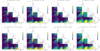 |
Fig. 6. Same as Fig. 3 but for the gSa in the prograde and retrograde encounter. |
| In the text | |
|
Fig. 7. Parameter space overlapped with true and false streams detected by COSTA for both early- and late-type galaxies, in the standard configurations (2000 particles and Δv = 40 km s−1) for three cases (gE0, gSa prograde, and gSa retrograde), but using different reliability thresholds. |
| In the text | |
|
Fig. 8. Simulated data points for one Monte Carlo realization, with NGC 1399 at the origin of coordinates. NGC 1404 is just below the cD (X ∼ −5, Y ∼ −5), and NGC 1387 is at X ∼ −20 arcmin. The positions of the three galaxies are indicated by black squares. |
| In the text | |
|
Fig. 9. Phase space of one Monte Carlo simulation. On the x-axis, we plot the distance from NGC 1399 in arcminutes, and on the y-axis we plot the velocities of the points in km s−1. The continuous solid and dashed-dotted lines represent the ±3σp profiles of the GCs and PNe, respectively, extracted from P+18 (their Fig. 9). The dashed black horizontal line represents the systemic velocity of NGC 1399 (1425 km s−1). |
| In the text | |
|
Fig. 10. Reliability map for Fornax cluster obtained with a reliability threshold of 70%. |
| In the text | |
|
Fig. 11. Stream (red points) and spurious structures (cyan points) overlapped on Fornax cluster reliability maps in the different shells (left columnR = 5′−7′; middle column R = 7′−12′; right column R = 12′−18′) and for the three different simulated streams (top: stream 1, middle: GalMer 1, and bottom GalMer 2). |
| In the text | |
|
Fig. 12. Density plot in Nmin − σ diagram, and number counts of the recovered artificial streams for the middle shell (i.e., 7′−12′) for stream 1 (top), GalMer 1 (middle), and GalMer 2 (bottom). The horizontal dashed line shows the true velocity dispersion of each stream. The sample was cleaned by using FN = 0.5 as the threshold in the n − Nmin space. Data were smoothed using a Gaussian kernel with a bandwidth equal to 3. |
| In the text | |
|
Fig. 13. Contaminant Fraction as a function of setup parameters for R = 5′−7′ shell (left column), R = 7′−12′ shell (middle column), and R = 12′−18′ shell (right column). Red points are for the GalMer 1 stream, green points for the GalMer 2 stream, and the blue points are for stream 1. |
| In the text | |
|
Fig. 14. Observed completeness (full dots) and true completeness (transparent triangles) as a function of the setup parameters for R = 5′−7′ shell (left column), R = 7′−12′ shell (middle column), and R = 12′−18′ shell (right column). The color-code is the same as in Fig. 13: red points for GalMer 1, green points for GalMer 2, and blue points for stream 1. |
| In the text | |
Current usage metrics show cumulative count of Article Views (full-text article views including HTML views, PDF and ePub downloads, according to the available data) and Abstracts Views on Vision4Press platform.
Data correspond to usage on the plateform after 2015. The current usage metrics is available 48-96 hours after online publication and is updated daily on week days.
Initial download of the metrics may take a while.