| Issue |
A&A
Volume 644, December 2020
|
|
|---|---|---|
| Article Number | A157 | |
| Number of page(s) | 6 | |
| Section | Planets and planetary systems | |
| DOI | https://doi.org/10.1051/0004-6361/202038746 | |
| Published online | 15 December 2020 | |
Radio observations of HD 80606 near planetary periastron
II. LOFAR low band antenna observations at 30–78 MHz
1
Hamburger Sternwarte, Universität Hamburg, Gojenbergsweg 112,
21029 Hamburg, Germany
e-mail: This email address is being protected from spambots. You need JavaScript enabled to view it.
2
INAF – Istituto di Radioastronomia, Via P. Gobetti 101,
Bologna, Italy
3
Jet Propulsion Laboratory, California Institute of Technology, 4800 Oak Grove Dr., M/S 67-201, Pasadena,
CA
91109, USA
4
MIT Haystack Observatory, 99 Millstone Rd.,
Westford, MA
01886, USA
Received:
25
June
2020
Accepted:
10
November
2020
Abstract
Context. All the giant planets in the Solar System generate radio emission via electron cyclotron maser instability, giving rise most notably to Jupiter’s decametric emissions. An interaction with the solar wind is at least partially responsible for all of these Solar System electron cyclotron masers. HD 80606b is a giant planet with a highly eccentric orbit, leading to predictions that its radio emission may be enhanced substantially near periastron.
Aims. This paper reports observations with the Low Frequency Array (LOFAR) of HD 80606b near its periastron in an effort to detect radio emissions generated by an electron cyclotron maser instability in the planet’s magnetosphere.
Methods. The reported observations are at frequencies between 30 and 78 MHz, and they are distinguished from most previous radio observations of extrasolar planets by two factors: (i) they are at frequencies near 50 MHz, much closer to the frequencies at which Jupiter emits (ν < 40 MHz) and lower than most previously reported observations of extrasolar planets; and (ii) sensitivities of approximately a few millijanskys have been achieved, an order of magnitude or more below nearly all previous extrasolar planet observations below 100 MHz.
Results. We do not detect any radio emissions from HD 80606b and use these observations to place new constraints on its radio luminosity. We also revisit whether the observations were conducted at a time when HD 80606b was super-Alfvénic relative to the host star’s stellar wind, which experience from the Solar System illustrates is a state in which an electron cyclotron maser emission can be sustained in a planet’s magnetic polar regions.
Key words: planets and satellites: individual: HD 80606b / radio continuum: planetary systems / planet–star interactions / planets and satellites: magnetic fields
© ESO 2020
1 Introduction
Giant planets in the Solar System generate radio emission as a result, at least partially, of the interaction between the solar wind and the planet’s magnetospheres. The solar wind impinging on a planet’s magnetosphere can generate currents in the planet’s magnetic polar regions, where an electron cyclotron maser is produced. There is a rich literature on the relevant processes, based substantially on in situ observations by spacecraft, and straightforward extrapolations predict that the same processes could occur in extrasolar planetary systems (e.g., Winglee et al. 1986; Zarka et al. 1997, 2001; Farrell et al. 1999; Bastian et al. 2000; Zarka 2007). The detection of magnetospherically generated radio emission in these systems would be the first direct detection of magnetic fields in extrasolar planets.
Radio emissions from extrasolar planets have been extensively searched for at frequencies ranging from 25 to 1400 MHz, with most of these observations having focused on “hot Jupiters,” massive planets in orbits with small semi-major axes and low eccentricities; both Zarka et al. (2015) and Lazio et al. (2016) contain extensive summaries of observational results. Sensitivities (1σ) obtained in past searches for extrasolar planetary magnetospheric emission have ranged from roughly 1000 mJy to below 1 mJy, with generally better sensitivities obtained at the higher frequencies. Typically, these sensitivities have not been sufficient to challenge the predicted levels, though some multi-epoch 74 MHz observations of τ Boo b (Lazio & Farrell 2007) do indicate that its emission is not consistent with the most optimistic predictions, if it does emit at that frequency. Recently, Vedantham et al. (2020) reported low radio frequency emission from the quiescent late-type star GJ 1151. The characteristics of this emission are consistent with it being generated by a sub-Alfvénic flow into the star’s magnetic polar regions, potentially from an orbiting terrestrial-mass planet. While exciting (and these observations would be sensitive to similar kinds of emission), such emissions do not clearly lead to constraints on the properties of the planet itself.
Moreover, existing estimates regarding the magnetic fields of hot Jupiters have considerable uncertainties, potentially at the level of more than an order of magnitude (e.g., France et al. 2010; Ekenbäck et al. 2010; Kao et al. 2016; Cauley et al. 2019; Yadav & Thorngren 2017). If hot Jupiter magnetic field strengths are comparable to, or weaker than, that of Jupiter, the range of frequencies over which their electron cyclotron masers would operate are unlikely to extend much above the range for Jupiter (≲40 MHz). Consequently, many of the existing observations may be at frequencies that are too high to detect extrasolar electron cyclotron maser emission (Vidotto et al. 2012).
The rationale behind the general focus on hot Jupiters has been twofold: if an extrasolar planet is close to its host star, the stellar wind should be more intense, with a concomitant increase in the strength of the planetary radio emission (Farrell et al. 1999; Zarka et al. 2001, 2018; Zarka 2007). Secondarily, planets close to their host stars produce the largest radial velocity signature, and, until the Kepler mission, the vast majority of extrasolar planets had been found with the radial velocity method.
An alternative line of investigation is to focus on highly eccentric extrasolar planets; the dramatic increases in stellar wind pressures that these planets experience near their periastrons should result in substantial enhancements in their radio luminosities (Gallagher & Dangelo 1981; Desch & Rucker 1983; Desch & Barrow 1984). A prototypical example is the giant planet HD 80606b (M = 3.94 ± 0.11 MJ, d = 66.6 pc), which has a111 day orbital period with one of the highest known orbital eccentricities (e = 0.9336 ± 0.0002; Fossey et al. 2009). Physical modeling of fluid bodies (the star and planet) in an eccentric orbit predicts that the planet should be driven into a state of pseudo-synchronized rotation (Hut 1981), with a rotational period of 39.9 h.
With a mass and a rotation period comparable to those of Jupiter, HD 80606b could reasonably be expected to emit at or above the frequencies at which Jupiter does (~40 MHz). Lazio et al. (2010) estimated that its emissions could extend as high as 55 MHz, and potentially to 90 MHz, when uncertainties on its mass and radius (i.e., bulk density) are considered. Comparing the sizes of the orbits of Jupiter and HD 80606b, and using what is known about the strength of the stellar wind of HD 80606b, Lazio et al. (2010) estimated the range of planetary luminosities during the course of its orbit. Near periastron, HD 80606b could reasonably be expected to be 3000 times as luminous as Jupiter, reaching a flux density of ~ 1 mJy when observed from Earth.
This paper reports observations of HD 80606b close to its periastron at a central frequency of 54 MHz (λ5.45 m). This work improves upon that of Lazio et al. (2010) in two aspects. First, it is both at a lower frequency, more comparable to that at which Jupiter emits, and it is more sensitive. Second, these observations include analyses of both the total and the circularly polarized intensities. An initial analysis of some of these data, using different methods, was presented by Knapp (2018), who obtained an rms noise of 6 mJy beam−1. In Sect. 2, we summarize the observations and data analyses, in Sect. 3 we present our results, and in Sect. 4 we discuss the results in context and present our conclusions.
2 Observations and analysis
Table 1 presents the observing log. The observations consist of five epochs that occurred during Low Frequency Array (LOFAR) Cycle 4. The observing strategy was to obtain a reference observation, near apoastron, to serve as a baseline observation. There are two observations prior to periastron, occurring approximately 48 and 18 h prior, and two observations subsequent to periastron, occurring approximately 48 and 18 hr after. Observations following periastron were conducted to allow for the possibility that an increase in planetary radio luminosity lags the increase in incident stellar wind. The combined uncertainties in the orbital periods and times of periastron typically amount to less than 0.1 days (about 2 h).
Observations at periastron were not conducted. While such observations would have the maximum incident stellar wind flux, there is the risk that the plasma frequency of the stellar wind could be larger than the planet’s electron cyclotron frequency (Weber et al. 2017). If so, the planetary radio emission would not be able to escape from the system.
HD 80606b observing log.
2.1 Data acquisition
All observations were acquired using LOFAR’s Low Band Array (LBA, van Haarlem et al. 2013), with the 30–75 MHz tuning used. The use of this frequency range maximizes the sensitivity by excluding the top and bottom of the band where the dipole response is suppressed.
Each LOFAR LBA station consists of 96 crossed dipoles; however, for Dutch stations (core and remote), only 48 dipoles can be used simultaneously due to hardware limitations at the station level. For these observations, the “LBA Outer” configuration was used, inwhich only the data from the outer 48 dipoles are recorded. The Outer configuration simplifies the calibration by reducing theprimary beam size, and the dipoles cross-talk. The primary beam for this configuration varies from approximately 3° to 5° across the band; we adopted a fiducial value of approximately 4° (full width at half maximum).
We used 23 core stations and 14 remote stations. International stations were not included in order to maintain a reasonable data volume and because subarcsecond resolution was not crucial. The longest baseline was therefore approximately 100 km, providing a nominal resolution at mid-band (54 MHz) of 12′′.
The observations were conducted in multi-beam mode, with one beam continuously pointing at a calibrator (3C 196) and one beam continuously pointing at the target (HD 80606b). Data were acquired in 244 subbands, of width 0.195 MHz, with 64 frequency channels per subband (3 kHz per frequency channel). During correlation, an integration time of 1 s and a frequency resolution of 3 kHz (i.e., the native resolution of the subband frequency channels) were used. After Radio Frequency Interference (RFI) detection, data were averaged down to 4 s and four frequency channels per subband, each with a bandwidth of 48 kHz.
2.2 Data reduction
The processing of the calibrator visibility data generally followed the procedures described previously by de Gasperin et al. (2019). The calibrator visibilities were used to isolate a number of systematic effects that were then applied to the target data. These effects are the amplitude bandpass, the stations’ clocks drifts, and the polarization delay between the X and Y dipoles. Together with these effects, an analytic estimation of the dipole beam effect on both amplitudes and phases was applied to the target data (van Haarlem et al. 2013).
The self-calibration starts by obtaining an initial sky model from available surveys: TGSS (Intema et al. 2017), NVSS (Condon et al. 1998), WENSS (Rengelink et al. 1997), and VLSS (Lane et al. 2014). Using sources from these surveys, we estimated their spectral indices, where possible up to the second order, and extrapolated them to the LBA frequency range. An average total electron content (TEC) above the target field was estimated for each antenna and time step. Uncertainties in the estimated TEC, and the resulting phase and delay uncertainties, are the strongest systematic effect still present in the data at this stage of the calibration. Once corrected, we can estimate the Faraday rotation and second-order beam effects. Sources in the first side lobe were imaged and subtracted from the data before starting a direction-dependent calibration.
The final direction-dependent calibration followed de Gasperin et al. (2020). Here, the best available model was divided into “direction-dependent calibrators” (DDcals), a compact group of sources on the sky, each of which accounts for at least 2 Jy of flux density. In this case, we used seven DDcals. For each DDcal, a direction-dependent solver (Offringa et al., in prep.) present in DP31 estimated the direction-dependent component of the TEC along the direction connecting each DDcal to each station. Finally, the field-of-view was imaged in facets with wsclean (Offringa et al. 2014), applying the correction estimated from the closest DDcal. The combined observations produced the deepest image ever made at ultra-low frequencies, with sensitivities of 800 μJy beam−1 in the Stokes I parameter and 700 μJy beam−1 in the Stokes V parameter.
Image sensitivities and inferred planetary radio luminosity limits.
3 Results
After removing the best estimation of systematic effects for each epoch, we imaged each independently, combining all data within an epoch in order to improve the signal-to-noise ratio. For each epoch, we imaged the entire band (30–78 MHz) as well as only the lower half (30–54 MHz). The motivation for imaging only the lower half of the band is that Jupiter’s radio emission truncates sharply above its cutoff frequency (≈ 40 MHz); combining all of the data across the entire frequency band risks decreasing the signal-to-noise ratio for any HD 80606b radio emission if its cutoff frequency occurs in the lower half of the band. Images were produced in both Stokes I and V parameters as the electron cyclotron maser instability is highly circularly polarized (e.g., Treumann 2006; Vorgul et al. 2011).
At no epoch do we find evidence for radio emission from HD 80606b. Table 2 summarizes the parameters of the images produced and the upper limits on the radio luminosity of the planet for each epoch, estimated using the full bandwidth (central frequency 54 MHz) and for the bottom half (central frequency 42 MHz). Variations in the image noise levels from epoch to epoch result from observing them at different elevations and from the changing of ionospheric conditions from day to day. At each epoch we estimated a “global” rms noise level, using all non-source pixels in the image, and a “local” rms noise level, determined from an annulus with inner radius 1′ and outer radius 3′ centered around the nearby radio source FIRST J092239.6+503529 (see Fig. 1). Figure 1 presents the Stokes I and V images of the HD 80606 field for the reference epoch of 2015 August 30. For all images, the synthesized beam diameter was approximately 30′′ × 15′′.
Due to the reduced bandwidth, we expected the image noise levels for the lower half of the band to be approximately 40% higher than those across the full band. In practice, we find that the noise levels in the lower half of the band are closer to 60% higher, a difference that we attribute to the lower sensitivity of the LBA dipoles in that frequency range (van Haarlem et al. 2013)combined with an increased level in RFI at lower frequencies and residual ionospheric calibration uncertainties producing larger effects at lower frequencies.
4 Discussion and conclusions
The results summarized in Table 2 are distinguished from previous observations of HD 80606b specifically and most other radio observations of extrasolar planets generally by two factors: (i) they areat frequencies near 50 MHz, much closer to the frequencies at which Jupiter emits (ν < 40 MHz) and, with the exception of observations by the Clark Lake Radio Observatory (Yantis et al. 1977) and the Ukrainian T-shaped Radio telescope (UTR-2, Ryabov et al. 2004), lower than most previously reported observations of extrasolar planets; and (ii) sensitivities of approximately a few millijanskys have been achieved, an order of magnitude or more below nearly all previous extrasolar planet observations below 100 MHz (see Fig. 2).
Lazio et al. (2010) estimated that the radio luminosity of HD 80606b could be as much as a factor of 3000 higher due to its much smaller distance to its host star as compared to Jupiter. The peak radio luminosity of Jupiter can reach 2 × 10¹⁸ erg s−1 near 40 MHz (Zarka et al. 2004); therefore, the radio luminosity of HD 80606b might be as much as 6 × 10²¹ erg s−1.
Implicit in the original analysis by Lazio et al. (2010) and in our discussion heretofore has been that the interaction between the HD 80606 stellar wind and the (assumed) magnetosphere of HD 80606b is super-Alfvénic, akin to the solar wind-planetary magnetosphere interaction for all the giant planets in the Solar System. If the interaction is sub-Alfvénic, the planet’s magnetosphere does not sustain a bow shock. In a sub-Alfvénic interaction, energy flows toward both the star and the planet are expected (e.g., Ip et al. 2004; Preusse et al. 2005, 2006; Willes & Wu 2005), but whether an electron cyclotron maser instability could be sustained in the planet’s polar regions is unclear. This scenario has been discussed at length, considering both Solar System bodies and extrasolar planets (Zarka et al. 2001; Preusse et al. 2006; Zarka 2007; Saur et al. 2013). Specifically, Saur et al. (2013) appear to have considered the conditions for HD 80606b when it was near apastron instead of the conditions appropriate for these observations, namely near periastron.
We now assess whether the interaction between HD 80606 stellar wind and the (assumed) magnetosphere of HD 80606b is likely to be super-Alfvénic or not. From the NASA Exoplanet Archive, the properties of HD 80606 are approximately solar, with M = 1.018 M⊙, R = 1.037 R⊙, and age ≈ 5.9 Gyr (Bonomo et al. 2017), and, given the various uncertainties, we henceforth treat it as equivalent to the Sun. At the time of the observations, the planet was at a distance of about 6.5 stellar radii, equivalent to approximately 0.03 au (Zarka 2007). At this distance, the solar wind has a plasma mass density of about 2 × 10⁻²⁰ g cm3 (Köhnlein 1996), the magnetic field is about 10−2 G, and the solar wind velocity is about 100 km s−1. The equivalent Alfvén velocity is about 220 km s−1.
The orbital velocity of HD 80606b at this phase in its orbit is approximately 250 km s−1. In contrast to hot Jupiters, which have essentially circular orbits at similar distances from their host stars, HD 80606b will have a nearly radial velocity. Thus, the equivalent velocity at which the stellar wind impacts the magnetosphere is approximately 350 km s−1. We conclude that the stellar wind-planet (magnetosphere) interaction is likely to be (moderately) super-Alfvénic and that an electron cyclotron maser instability could be sustained at least pre-periastron. Post-periastron, as the planet recedes from the star, there may be intervals during which the interaction becomes sub-Alfvénic.
By conducting observations in the 30–78 MHz band, this work has addressed one of the major uncertainties present in most previous efforts to detect the radio emission from extrasolar planets. While there have been a number of relatively sensitive searches conducted, these have typically been at frequencies above 100 MHz, in comparison to Jupiter’s upper frequency for emission of approximately 35 MHz. Furthermore, as discussed in Lazio et al. (2010), estimates of the upper emission frequency for HD 80606b are between 55 and 90 MHz, based on determinations of various planetary parameters and scaling laws.
Broadly speaking, many of the considerations for the observations of HD 80606b that were described by Lazio et al. (2010) remain valid today. HD 80606b remains the planet with the second-highest known orbital eccentricity. While HD 7449b has since been discovered (e = 0.92, Dumusque et al. 2011; Wittenmyer et al. 2019), of the planets with the highest orbital eccentricities, HD 80606b remains the one with the shortest orbital period (thereby facilitating more opportunities for observation), and none of those planets have distances significantly shorter than HD 80606b; HD 20782b (e = 0.95) is at a distance of 36 pc, resulting in less than a factor of four improvement in potential radio luminosity limits relative to HD 80606b. Fomalhaut b has a significant orbital eccentricity (e = 0.87) and has the virtue of being significantly closer (≈7.7 pc), but its notional orbital period is so long (≈1500 yr) and its semi-major axis so large (160 au) that it is not a practical target. Furthermore, recent observations have questioned its nature (Gáspár & Rieke 2020). Similarly, no revolutionary improvements in observational capability seem to be coming in the near term, with the exception of the completion of NenuFAR (Zarka et al. 2020) and the LOFAR upgrade (LOFAR 2.0). LOFAR 2.0, planned to be operational by 2024, aims to improve the sensitivity of the LBA system, doubling the usable dipoles of LOFAR at frequencies below 100 MHz. Another improvement will come with the simultaneous observations with the LOFAR HBA system, which will be crucial for modeling ionospheric disturbances and removing their effect from LBA data. Unfortunately, the Sun is moving from the solar cycle minimum to maximum, which will likely lead to an interval of higher ionospheric activity that will make ultra-low frequency observations more challenging. When the LOFAR 2.0 system is fully operational, these limits may be able to be improved by as as much as a factor of five.
The low radio frequency component of the Square Kilometre Array (SKA1-Low) will likely not be fully operational until the end of the 2020s, and its site in Western Australia means that it will not be able to observe HD 80606b, though it could observe many of the other highest-eccentricity planets. Near-term space-based radio telescopes, such as the Sun Radio Interferometer Space Experiment (SunRISE; Kasper et al. 2019), will likely not have the sensitivity to detect extrasolar planetary radio emission, unless it becomes significantly stronger at frequencies below 20 MHz; if future space-based radio telescopes are larger, they may be sensitive enough to detect such emissions.
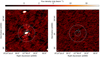 |
Fig. 1 Images of the immediate surroundings of HD 80606, for the full band (30–78 MHz). The location of the star is at the center of the cross-hair. The annulus traced by the dashed line is the region used to estimate the local rms noise. Contours start at 3σ with σ = 800 μJy beam−1. The beam, 28′′ × 14′′, is shown in the bottom-left corner of the image. The source just to the south of the star’s location is FIRST J092239.6+503529. Left: Stokes I image. Right: Stokes V image, corresponding to the Stokes I image shown in the left-hand panel. |
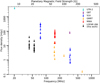 |
Fig. 2 Upper limits for direct observation of radio emission from extrasolar planets. In black, we show the results presented in this paper at a 3σ confidence level. For reference, at the distance of HD 80606b, the burst emission of Jupiter would be weaker than 0.1 mJy. |
Acknowledgements
We thank A. Vidotto for helpful discussions about solar wind models, D. Winterhalter and W. Farrell for the support in writing the initial LOFAR proposal, and the referee for several comments that clarified both the content and presentation of this work. This work is partly funded by the Deutsche Forschungsgemeinschaft under Germany’s Excellence Strategy EXC 2121 “Quantum Universe” 390833306. Part of this research was carried out at the Jet Propulsion Laboratory, California Institute of Technology, under a contract with the National Aeronautics and Space Administration. A portion of this work was funded by the NASA Lunar Science Institute (via Cooperative Agreement NNA09DB30A). This research has made use of the NASA Exoplanet Archive, which is operated by the California Institute of Technology, under contract with the National Aeronautics and Space Administration under the Exoplanet Exploration Program. This research has made use of NASA’s Astrophysics Data System Bibliographic Services. LOFAR is the LOw Frequency ARray designed and constructed by ASTRON. It has observing, data processing, and data storage facilities in several countries, which are owned by various parties (each with their own funding sources), and are collectively operated by the ILT foundation under a joint scientific policy. The ILT resources have benefitted from the following recent major funding sources: CNRS-INSU, Observatoire de Paris and Universite d’Orleans, France; BMBF, MIWF-NRW, MPG, Germany; Science Foundation Ireland (SFI), Department of Business, Enterprise and Innovation (DBEI), Ireland; NWO, The Netherlands; The Science and Technology Facilities Council, UK; Ministry of Science and Higher Education, Poland; Istituto Nazionale di Astrofisica (INAF).
References
- Bastian, T. S., Dulk, G. A., & Leblanc, Y. 2000, ApJ, 545, 1058 [NASA ADS] [CrossRef] [Google Scholar]
- Bonomo, A. S., Desidera, S., Benatti, S., et al. 2017, A&A, 602, A107 [NASA ADS] [CrossRef] [EDP Sciences] [Google Scholar]
- Cauley, P. W., Shkolnik, E. L., Llama, J., & Lanza, A. F. 2019, Nat. Astron., 3, 1128 [CrossRef] [Google Scholar]
- Condon, J. J., Cotton, W. D., Greisen, E. W., et al. 1998, AJ, 8065, 1693 [Google Scholar]
- de Gasperin, F., Dijkema, T. J., Drabent, A., et al. 2019, A&A, 5, A5 [NASA ADS] [CrossRef] [EDP Sciences] [Google Scholar]
- de Gasperin, F., Brunetti, G., Brüggen, M., et al. 2020, A&A, 642, A85 [CrossRef] [EDP Sciences] [Google Scholar]
- Desch, M. D., & Barrow, C. H. 1984, J. Geophys. Res., 89, 6819 [CrossRef] [Google Scholar]
- Desch, M. D., & Rucker, H. O. 1983, J. Geophys. Res., 88, 8999 [CrossRef] [Google Scholar]
- Dumusque, X., Lovis, C., Ségransan, D., et al. 2011, A&A, 535, A55 [NASA ADS] [CrossRef] [EDP Sciences] [Google Scholar]
- Ekenbäck, A., Holmström, M., Wurz, P., et al. 2010, ApJ, 709, 670 [NASA ADS] [CrossRef] [Google Scholar]
- Farrell, W. M., Desch, M. D., & Zarka, P. 1999, J. Geophys. Res., 104, 14025 [NASA ADS] [CrossRef] [Google Scholar]
- Fossey, S. J., Waldmann, I. P., & Kipping, D. M. 2009, MNRAS, 396, L16 [NASA ADS] [CrossRef] [Google Scholar]
- France, K., Stocke, J. T., Yang, H., et al. 2010, ApJ, 712, 1277 [NASA ADS] [CrossRef] [Google Scholar]
- Gallagher, D. L., & Dangelo, N. 1981, Geophys. Res. Lett., 8, 1087 [CrossRef] [Google Scholar]
- Gáspár, A., & Rieke, G. H. 2020, Proc. Natl. Acad. Sci., 117, 9712 [CrossRef] [Google Scholar]
- Hut, P. 1981, A&A, 99, 126 [NASA ADS] [Google Scholar]
- Intema, H. T., Jagannathan, P., Mooley, K. P., & Frail, D. A. 2017, A&A, 598, A78 [NASA ADS] [CrossRef] [EDP Sciences] [Google Scholar]
- Ip, W.-H., Kopp, A., & Hu, J.-H. 2004, ApJ, 602, L53 [NASA ADS] [CrossRef] [Google Scholar]
- Kao, M. M., Hallinan, G., Pineda, J. S., et al. 2016, ApJ, 818, 24 [NASA ADS] [CrossRef] [Google Scholar]
- Kasper, J., Lazio, J., Romero-Wolf, A., Lux, J., & Neilsen, T. 2019, IEEE Aerosp. Conf. Proc., 2019-March (IEEE Computer Society) [Google Scholar]
- Knapp, M. E. 2018, PhD thesis, Massachusetts Institute of Technology, Massachusetts, USA [Google Scholar]
- Köhnlein, W. 1996, Sol. Phys., 169, 209 [NASA ADS] [CrossRef] [Google Scholar]
- Lane, W. M., Cotton, W. D., van Velzen, S., et al. 2014, MNRAS, 440, 327 [NASA ADS] [CrossRef] [Google Scholar]
- Lazio, T. J. W., & Farrell, W. M. 2007, ApJ, 668, 1182 [NASA ADS] [CrossRef] [Google Scholar]
- Lazio, T. J. W., Shankland, P. D., Farrell, W. M., & Blank, D. L. 2010, AJ, 140, 1929 [NASA ADS] [CrossRef] [Google Scholar]
- Lazio, T. J. W., Shkolnik, E., Hallinan, G., & Planetary Habitability Study Team 2016, W. M. Keck Institute for Space Studies: Planetary Magnetic Fields: Planetary Interiors and Habitability [Google Scholar]
- Offringa, A. R., McKinley, B., Hurley-Walker, N., et al. 2014, MNRAS, 444, 606 [NASA ADS] [CrossRef] [Google Scholar]
- Preusse, S., Kopp, A., Büchner, J., & Motschmann, U. 2005, A&A, 434, 1191 [NASA ADS] [CrossRef] [EDP Sciences] [Google Scholar]
- Preusse, S., Kopp, A., Büchner, J., & Motschmann, U. 2006, A&A, 460, 317 [NASA ADS] [CrossRef] [EDP Sciences] [Google Scholar]
- Rengelink, R. B., Tang, Y., de Bruyn, a. G., et al. 1997, A&AS, 124, 259 [NASA ADS] [CrossRef] [EDP Sciences] [Google Scholar]
- Ryabov, V. B., Zarka, P., & Ryabov, B. P. 2004, Planet. Space Sci., 52, 1479 [NASA ADS] [CrossRef] [Google Scholar]
- Saur, J., Grambusch, T., Duling, S., Neubauer, F. M., & Simon, S. 2013, A&A, 552, A119 [NASA ADS] [CrossRef] [EDP Sciences] [Google Scholar]
- Treumann, R. A. 2006, A&ARv, 13, 229 [NASA ADS] [CrossRef] [Google Scholar]
- van Haarlem, M. P., Wise, M. W., Gunst, a. W., et al. 2013, A&A, 556, A2 [NASA ADS] [CrossRef] [EDP Sciences] [Google Scholar]
- Vedantham, H. K., Callingham, J. R., Shimwell, T. W., et al. 2020, Nat. Astron., 4, 577 [CrossRef] [Google Scholar]
- Vidotto, A. A., Fares, R., Jardine, M., et al. 2012, MNRAS, 423, 3285 [NASA ADS] [CrossRef] [Google Scholar]
- Vorgul, I., Kellett, B. J., Cairns, R. A., et al. 2011, Phys. Plasmas, 18, 056501 [CrossRef] [EDP Sciences] [PubMed] [Google Scholar]
- Weber, C., Lammer, H., Shaikhislamov, I. F., et al. 2017, MNRAS, 469, 3505 [NASA ADS] [CrossRef] [Google Scholar]
- Willes, A. J., & Wu, K. 2005, A&A, 432, 1091 [NASA ADS] [CrossRef] [EDP Sciences] [Google Scholar]
- Winglee, R. M., Dulk, G. A., & Bastian, T. S. 1986, ApJ, 309, L59 [NASA ADS] [CrossRef] [Google Scholar]
- Wittenmyer, R. A., Clark, J. T., Zhao, J., et al. 2019, MNRAS, 484, 5859 [NASA ADS] [CrossRef] [Google Scholar]
- Yadav, R. K., & Thorngren, D. P. 2017, ApJ, 849, L12 [NASA ADS] [CrossRef] [Google Scholar]
- Yantis, W. F., Sullivan, W. T. I., & Erickson, W. C. 1977, Bull. Am. Astron. Soc., 9, 453 [Google Scholar]
- Zarka, P. 2007, Planet. Space Sci., 55, 598 [NASA ADS] [CrossRef] [Google Scholar]
- Zarka, P., Queinnec, J., Ryabov, B. P., et al. 1997, Planetary Radio Emission IV, 101 [Google Scholar]
- Zarka, P., Treumann, R. A., Ryabov, B. P., & Ryabov, V. B. 2001, Ap&SS, 277, 293 [Google Scholar]
- Zarka, P., Cecconi, B., & Kurth, W. S. 2004, J. Geophys. Res. Space Phys., 109, A09S15 [Google Scholar]
- Zarka, P., Lazio, J., & Hallinan, G. 2015, Advancing Astrophysics with the Square Kilometre Array (AASKA14), 120 [CrossRef] [Google Scholar]
- Zarka, P., Marques, M. S., Louis, C., et al. 2018, A&A, 618, A84 [NASA ADS] [CrossRef] [EDP Sciences] [Google Scholar]
- Zarka, P., Denis, L., Tagger, M., et al. 2020, in International Union of Radio Science, General Assembly & Science Symposium 2020, URSI GASS 2020, Rome, Italy, http://www.ursi.org/proceedings/procGA20/papers/URSIGASS2020SummaryPaperNenuFARnew.pdf [Google Scholar]
All Tables
All Figures
|
Fig. 1 Images of the immediate surroundings of HD 80606, for the full band (30–78 MHz). The location of the star is at the center of the cross-hair. The annulus traced by the dashed line is the region used to estimate the local rms noise. Contours start at 3σ with σ = 800 μJy beam−1. The beam, 28′′ × 14′′, is shown in the bottom-left corner of the image. The source just to the south of the star’s location is FIRST J092239.6+503529. Left: Stokes I image. Right: Stokes V image, corresponding to the Stokes I image shown in the left-hand panel. |
| In the text | |
|
Fig. 2 Upper limits for direct observation of radio emission from extrasolar planets. In black, we show the results presented in this paper at a 3σ confidence level. For reference, at the distance of HD 80606b, the burst emission of Jupiter would be weaker than 0.1 mJy. |
| In the text | |
Current usage metrics show cumulative count of Article Views (full-text article views including HTML views, PDF and ePub downloads, according to the available data) and Abstracts Views on Vision4Press platform.
Data correspond to usage on the plateform after 2015. The current usage metrics is available 48-96 hours after online publication and is updated daily on week days.
Initial download of the metrics may take a while.