| Issue |
A&A
Volume 643, November 2020
|
|
|---|---|---|
| Article Number | A109 | |
| Number of page(s) | 8 | |
| Section | Interstellar and circumstellar matter | |
| DOI | https://doi.org/10.1051/0004-6361/202039183 | |
| Published online | 10 November 2020 | |
Color–color diagrams as tools for assessment of the variable absorption in high mass X-ray binaries
1
Institut für Astronomie und Astrophysik, Universität Tübingen,
Sand 1,
72076
Tübingen, Germany
e-mail: grinberg@astro.uni-tuebingen.de
2
Physics Department, CB 1105, Washington University,
One Brookings Drive,
St. Louis,
MO
63130-4899, USA
3
Lawrence Livermore National Laboratory,
7000 East Avenue,
Livermore,
CA
94550, USA
Received:
14
August
2020
Accepted:
1
October
2020
High mass X-ray binaries hold the promise of allowing us to understand the structure of the winds of their supermassive companion stars by using the emission from the compact object as a backlight to evaluate the variable absorption in the structured stellar wind. The wind along the line of sight can change on timescales as short as minutes and below. However, such short timescales are not available for the direct measurement of absorption through X-ray spectroscopy with the current generation of X-ray telescopes. In this paper, we demonstrate the usability of color–color diagrams for assessing the variable absorption in wind accreting high mass X-ray binary systems. We employ partial covering models to describe the spectral shape of high mass X-ray binaries and assess the implication of different absorbers and their variability on the shape of color–color tracks. We show that in taking into account, the ionization of the absorber, and in particular accounting for the variation of ionization with absorption depth, is crucial to describe the observed behavior well.
Key words: stars: winds, outflows / stars: massive / X-rays: binaries
© ESO 2020
1 Introduction
In high mass X-ray binaries (HMXBs), the compact object, whether a black hole or neutron star, accretes from a massive stellar companion. In particular, in Supergiant X-ray binaries, as opposed to Be X-ray binaries, the stellar companion is a giant O or B type star whose strong stellar wind feeds the accretion (for a review, see Martínez-Núñez et al. 2017). The winds of such stars are line-driven and thus not smooth, but they are highly structured, with dense pockets (“clumps”) of gas embedded in a rarefied medium (e.g., Owocki & Rybicki 1984; Feldmeier 1995). Observations imply that the clumping already starts close to the stellar surface, within less than r ≲ 0.25 R⋆ (Cohen et al. 2011; Torrejón et al. 2015), that is to say closer than the typical observed locations of the compact objects. Additionally, the presence of the compact object can lead to the formation of large-scale structures in the wind, such as photoionization and accretion wakes or focused wind components (Blondin et al. 1990).
Understanding the clumpy structure of O/B stellar winds is crucial, both for understanding the mass loss, and thus evolution, of the O/B stars themselves (Fullerton et al. 2006) and in order to understand accretion processes in HMXBs (Martínez-Núñez et al. 2017). Accretion of individual clumps could lead to the observed flares in both persistent HMXBs (e.g., Fürst et al. 2010; Martínez-Núñez et al. 2014; García et al. 2018) and supergiant fast X-ray transients (SFXTs; e.g, Bozzo et al. 2011; Ferrigno et al. 2020). Clumps passing through the line of sight toward the compact object, on the other hand, lead to discrete absorption events (e.g., Bałucińska-Church et al. 2000; Naik et al. 2011; Yamada et al. 2013; Hemphill et al. 2014; Hirsch et al. 2019).
Models and simulations of the clumpy structure of O/B winds (e.g., Oskinova et al. 2012; Sundqvist & Owocki 2013; Sundqvist et al. 2018) exist, as do simulations of clumpy wind accretion onto compact objects (El Mellah et al. 2018) and variable absorption in a clumpy wind environment (Grinberg et al. 2015; El Mellah et al. 2020). However, the variability timescales predicted are usually too short to allow current X-ray instruments to accumulate spectra of a quality that would allow one to constrain the absorption during the passage of a single clump well. For example, Grinberg et al. (2017) used the setup of El Mellah et al. (2018) to calculate that the correlation time between the peaks of the variable column density for the neutron star HMXB Vela X-1 is at most 1 ks, or equivalently only a few self-crossing times of the wind clumps. A more thorough exploration of parameter space of different wind properties in toy models shows that absorption measurements on timescales of a few hundred seconds hold the potential to allow measurements of clump size and mass (El Mellah et al. 2020). While light curves and hardness ratios during dipping show variability on such timescales and below (Grinberg et al. 2017; Hirsch et al. 2019), the periods are too short to accumulate spectra that are well and directly measure the absorption in a single dip event of a few 100 s length or below from the current instruments’ spectra.
However, where not enough information is available for a full spectral analysis, the location in (X-ray) color–color space can be used to obtain information about spectral properties. Similar approaches have been employed when analyzing faint sources and, for example, when trying to understand source populations in other galaxies or contributions from different emission components (e.g., Carpano et al. 2005). The advantage of HMXBs is that the underlying spectral shape of the continuum emission from the compact object can often be well constrained from time-averaged spectra, especially when data at high energies not affected by absorption (≳10 keV) are available, allowing for better constraints on the expected location in color–color space.
The aim of this paper is thus to connect the shape of tracks on color–color tracks with absorption variability in HXMBs. It builds upon previous work of Nowak et al. (2011) and Hanke (2011), who attempted to describe the color–color tracks of neutral absorbers, and expands on this previous work with more realistic, ionized absorbers that are a better description for the hot, structured winds of O/B stars. We first discuss the observational signatures of dipping in wind-accreting HMXBs and partial covering models often used to describe HMXB spectra in Sect. 2. We then revisit variable neutral absorber models in Sect. 3, where we additionally discuss the influence of the covering fraction and changes in the underlying spectral shape on the shape of color–color tracks. In Sect. 4, we discuss the effects of a warm absorber and in particular the effects of a warm absorber whose ionization depends on its equivalent hydrogen column density, as would be expected in a wind environment with clumps or other overdensities. We finish with a summary and outlook in Sect. 5.
2 Signatures of dipping in wind-accreting HMXBs
2.1 Observational patterns
Short, pronounced increases of absorption, often called dips, have been observed in a number of wind-accreting HMXB sources, such as Cyg X-1 (e.g., Li & Clark 1974; Bałucińska-Church et al. 2000; Hirsch et al. 2019), Vela X-1 (Odaka et al. 2013; Grinberg et al. 2017), and 4U 1538−52 (Hemphill et al. 2014). As opposed to off states, which are interpreted as the cessation of accretion, the underlying continuum does not change during dips and the spectral variability is driven by changes in the absorbing column. The length of such absorption episodes ranges from tens of seconds to kiloseconds and above, with the longer dipping episodes often showing a pronounced temporal substructure.
So far, color–color diagrams have been mainly used to disentangle the absorption level in the bright HMXB Cyg X-1 with a variety of different X-ray instruments (Nowak et al. 2011; Miškovičová et al. 2016; Basak et al. 2017; Hirsch et al. 2019). It is the most prominent example as it is bright and well studied as a key source for understanding both stellar winds in HMXBs and the physics of accretion onto black holes. Both Nowak et al. (2011) and Hanke et al. (2008) attempted to provide, with some success, a physical description of the color–color tracks based on Suzaku and Chandra observations, respectively, with a partial covering model (see Sect. 2.2). However, discrepancies between the observations and data remain; in particular, the curve of the data is more pointy than that of the model. Nowak et al. (2011) attributed this to the possible influence of ionization, but did not attempt to include an ionized absorber in their models. From high resolution spectra, the presence of an ionized absorber has been shown by Hanke et al. (2009) and Miškovičová et al. (2016) and its variability with an increasing level of absorption can be seen in Hirsch et al. (2019). We note that Hirsch et al. (2019) used color–color diagrams to divide their observation into different absorption levels; however, they describe the shape of the tracks with an empirical polynomial model only.
2.2 Partial covering model
The simplest assumption for a HMXB spectrum is a continuum modified by a partially covering absorber, that is, only a certain percentage (the covering fraction, fc) of the X-rays emitted by the central source are absorbed locally while the rest of them (1 − fc) arrive at the observer modified by interstellar absorption only. Such models have been used widely in the literature to describe HMXBs (e.g., Fürst et al. 2014; Fornasini et al. 2017). The partial covering can be realized in the following different ways. Firstly, for partial covering in space, the absorber covers only a part of the emitting region. This could be the case for a relatively small, compact absorber and/or an emission region that is extended when compared to the absorber. Secondly, for partial covering in time, any observation averages over some exposure time. If the absorber changes during this time, as would be expected given the quick dynamic timescales of both structured stellar wind and accretion streams, the observed emission is the sum of spectra with different levels of absorption. Thirdly, for dust scattering (e.g., Xu et al. 1986, and references therein), the spectrum consists of a directly observed component that is subject to local absorption events and a somewhat time-delayed and averaged (due to scatterings at different radii) spectrum from the dust scattering halo. This spectrum is softer than the direct emission due to the energy-dependency of the scattered emission. The situation may be further complicated through the existence, in some sources, of asoft excess component, whose origin is still often unclear (e.g., Hickox et al. 2004) and which may be affected by absorption differently than the primary continuum components. This soft excess includes possible contributionfrom a photoionized wind component, where a forest of unresolved fluorescence lines could contribute to the overall soft emission on scales much larger than the point-like emission from the vicinity of the compact object.
A basic model to describe partial covering can be written as:
 (1)
(1)
where absism is the absorption in the interstellar medium (ISM), continuum is the continuum emission, 0 ≦ f ≦ 1 is the covering fraction, and abswind is the local absorption in the system, that is, in the (disrupted) stellar wind of the companion. This basic model for a partial coverer best represents spatial covering in space or time, as dust scattering would result in additional softening of the uncovered emission component.
For the continuum at energies ≲10 keV, a power law usually offers a good description. In general, physical models for the X-ray continuum emission in HMXBs, usually from highly magnetized neutron stars, are rare and the continuum is described empirically by power laws, which are modified by different breaks and cutoffs, or Comptonization models that are power-law shaped. Similar empirical descriptions can be employed for black hole accretors.
Such a model for a partial covering can be easily set up in the most current X-ray analysis environments; in our work we use the Interactive Spectral Interpretation System (ISIS) version 1.6.2 (Houck & Denicola 2000; Houck 2002; Noble & Nowak 2008). Here and in the remainder of the paper, we discuss the effects of a partial coverer using a power law continuum – such a simple continuum description has been used repeatedly in the literature to describe the continuum spectral shape of HMXBs below 10 keV (e.g., Hemphill et al. 2014; Miškovičová et al. 2016; Grinberg et al. 2017). Realizations of Eq. (1) for a covering fraction f = 90% and different values of local absorption are shown in Fig. 1, which follows a similar illustration in Hirsch et al. (2019).
For color–color diagrams, we consider the fractions (“colors”) between the fluxes in three energy bands, with band 1 having the lowest and band 3 having the highest energies with a soft color 1/2 and a hard color 2/3. It can easily be seen in Fig. 1 that the value of a given color is not a monotonic function of absorption strength. In particular, the soft color 1/2 is similar when the local absorber abswind is absent and when the local, partially covering absorption is very strong and such a strong absorber removes all covered flux in bands 1 and 2, leaving just the contribution of the uncovered component.
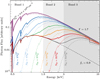 |
Fig. 1 Principle demonstration of the effect of a variable partial covering absorption on an absorbed powerlaw with photon index Γ = 1.7 and ISM absorption |


3 A variable neutral absorber
Here, we introduce the tracks that a source traces in the color–color diagram in the presence of a variable neutral absorber. Some effects of the variable neutral absorber on such tracks have been discussed in the previous works by Hanke et al. (2008), Nowak et al. (2011), and Hirsch et al. (2019) and we expand upon these first discussions by including the influence of short-term variability of a spectral shape of the underlying continuum.
3.1 Tracks on color–color diagrams
In the partial covering model presented in Sect. 2.2, there are the following three main parameters that define the shape of the spectrum and they can vary: the photon index Γ of the power law continuum, the absorbing column of the local absorber abswind, and the covering fraction f. The absorption in the interstellar medium, absism, is constant.
The photon index can show intrinsic variability on both short and long scales (e.g., Skipper et al. 2013; Grinberg et al. 2013; Fürst et al. 2014), although we point out that strong changes are usually associated with changes in emission geometry and thus they happen on longer timescales than those addressed in this work. In the clumpy wind or clumpy absorber paradigm, the local absorber can change strongly on short timescales of less than minutes, as clumps enter and leave the line of sight towardthe compact object (e.g., El Mellah et al. 2020). Short-term changes in the covering fraction are somewhat harder to realize, but they could be due to changing the number of clumps along the line of sight or the time delay between changes in the primary continuum and scattered component.
The exact shape of the tracks is always going to be dependent on a given instrument, even for the same spectral shape of the source. Here and in the following, when discussing general trends (Sects. 4.2.1 and 4.3.1), we calculate the tracks that such changes lead to in a color–color diagram using the example of a Chandra-HETGS/MEG observation of a bright source using typical value ranges for Γ and fc. We model the absorption with the updated version of the tbabs1 model (Wilms et al. 2000), using wilm (Wilms et al. 2000) cross-sections and vern abundances (Verner et al. 1996). We simulate observed spectra using real Chandra-HETGS/MEG responses (RMFs and ARFS), use the thusly simulated observations to calculate hardness values, and show the resulting tracks in Fig. 2.
Changes in individual parameters lead to typical changes in the color–color tracks: changes in the neutral absorption column density lead to typical curved or “nose-shaped” tracks (Fig. 2, left and middle), while changes in the covering fraction andintrinsic spectral shape show distinctly different patterns that could lead to some of the spread around the curves that observational data show (Fig. 3). If the underlying shape of the color–color track can be well modeled, such deviations can be potentially used to assess the variability of the underlying continuum and covering fraction on short timescales. As the driving observable is the actual shape of the nose-shaped track, we concentrate on changes in absorption column for the remainder of the paper.
3.2 Comparison to observed color–color tracks for Cyg X-1
A variable neutral absorber is a simple enough model that can be used to directly model observed color–color diagrams. Nowak et al. (2011) have presented fits of such a model to Suzaku data and Chandra-HETGS data have been discussed by Hanke et al. (2008) and Hanke (2011). In all cases, the model describes the overall trend of the shape of the tracks, but fails to reproduce the details; in particular, the curvature of the data is more pointy than the model.
For a comparison with the data, we use Chandra ObsID 3814, a ~50 ks observation taken in the TE graded mode on 2003 April 19 and covering the orbital phases 0.93–0.03, that is, at a phase where strong dipping is expected and indeed observed. To obtain lightcurves with a resolution of 25.5 s, we follow the standard extraction procedure, as was also done in Hirsch et al. (2019), for example. The high resolution spectrum of the non-dip phase of this observation has been previously analyzed by Hanke et al. (2009), whose analysis also includes the simultaneous broadband data taken with the RXTE satellite. Hanke et al. (2009) list different values in the range of 1.5–1.7 for the photon index of the power law used to describe the continuum and show the importance of coverage above ~10 keV to constrain the continuum shape, but they also emphasize the remaining uncertainties in spectral modeling. The high-resolution spectra of the Si and S regions of the observation have been analyzed by Hirsch et al. (2019) during dip and non-dip phases and for our theoretical predictions, we use the same MEG minus 1 order RMF and ARF files for non-dip phases as they did in their analysis.
To guide the eye, we first characterize the shape of the tracks using an empirical fit, in an approach similar to Hirsch et al. (2019) (Fig. 3, left panel). Specifically, we characterize the curve using a parameterized second-degree polynomial for each of the two colors. The best fit is obtained by minimizing the distance of each data point to the curve. The distances in either color are weighted with the respective uncertainty of each data point as in the definition of χ2 statistics.
We then turn to comparing the data with theoretical color–color tracks for a neutral absorber. The tracks for Γ = 1.6 are shown in the middle panel of Fig. 3. We also calculate the tracks for Γ = 1.5 and 1.7 andcompare them to the observations. This results in the expected slight shift of the tracks, mainly along the vertical axis (as expected from Fig. 2, middle panel), with Γ = 1.6 agreeing with the data best. The behavior we observe is consistent with the problems previously pointed out in the literature: The data is more pointy than the predictions. This deviation cannot be explained by the variability of the power law shape or covering fraction (cf. Fig. 2). Nowak et al. (2011) suggest that the deviation stems from the assumption of a neutral absorber: The wind material is intrinsically ionized to some level (e.g., Sander et al. 2018) and any material in the vicinity of the compact object is further ionized by its intense X-ray radiation. We discuss such an ionized absorber in the next section.
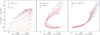 |
Fig. 2 Simulated color–color tracks for varying parameters of a partially absorbed power law model for HETG-MEG and parameter ranges typical for the HMXB Cygnus X-1. |
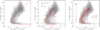 |
Fig. 3 Comparison of the color–color diagrams of the Chandra observation ObsID 3814 using the MEG M1 arm with different models. Left: empirical polynomial fit. Middle: neutral grid using the tbabs absorption model for different covering fractions and the same continuum photon index Γ = 1.6. Right: homogeneously ionized absorber using the warmabs model with continuum photon index Γ = 1.6 and a covering fraction of 0.95. The equivalent absorbing column density,NH, changes from 0.25 × 10⁻²² cm−2 to 32 × 10−22 cm−2 along each line, with each line showing the track for a different ionization parameter log ξ as indicated by the different colors. |
4 Warm, ionized absorbers
4.1 Modeling an ionized absorber
The ionization of the material local to the HMXB changes its X-ray absorbing properties. In the following, we assess how the change in ionization influences the tracks a source traces on the color–color diagram with variable absorption.
In order to do so, we use version 2.30 of the warmabs family of photoionization models (Kallman et al. 2009), which is a part of the XSTAR package (Bautista & Kallman 2001; Kallman & Bautista 2001), to model the ionized absorber. Figure 4 shows how the relative absorption as calculated by warmabs changes for the same equivalent hydrogen column density with a varying ionization parameter, log ξ, with
 (2)
(2)
for which Lx is the ionizing luminosity above 13.6 eV, n is the gas density, and r is the distance from the ionizing source (Tarter et al. 1969). The warmabs model can be used to access ionization parameters log ξ between −4.0 and 5.0. While the relative absorption decreases overall, the decrease in individual bands is a complex function of ionization due to contributions of different elements and ions (Fig. 4). We note that for the same column density, the lowest ionization of warmabs (logξ = −4.0) results in a stronger absorption than the neutral tbabs with abundances and cross-sections as discussed in Sect. 3.1. This difference is due to the different abundances and cross-sections used in the models.
To account for standard conditions and for ease of reproducibility, we use standard population files delivered with warmabs. In particular, we use the files that were pre-calculated for densities of 1012 cm−3, as these are typical densities of the smooth wind at the location of the compact object (Lomaeva et al. 2020) and as warmabs, using these population files, has been previously, successfully used to model the observations of Cyg X-1 during the non-dipping phase (Hanke 2011). However, we do note that densities in a structured wind can show a gradient up to a factor of 1000 and above (e.g., Sundqvist et al. 2018). Standard populations files are calculated for an illumination with a powerlaw with a photon index of Γ = 2. While this is softer than the Γ = 1.6 powerlaw that we employ here, the differences can be neglected given the broad energy bands used and further uncertainties, such as the above mentioned density gradients and the likely presence of a multiphase medium in wind-accreting HMXBs (e.g., Boroson et al. 2003; Grinberg et al. 2017; Lomaeva et al. 2020).
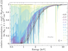 |
Fig. 4 Relative transmission in the 0.5–10 keV band for an equivalent hydrogen column density of NH = 2 × 1022 cm−2 and varyingionization parameters using warmabs shown in color. For comparison, neutral absorption as modeled with the tbabs model for the same hydrogen column density is shown in gray. |
4.2 Homogeneous warm absorber
4.2.1 Tracks on color–color diagrams
We calculate the tracks on the color–color diagrams for media of different ionization. Different ionization levels of the warm absorber lead to changes in the shape of the tracks in the color–color diagrams, as shown in Fig. 5. For the lowest ionization parameter, logξ = −4.0, the tracks are similar to those of a neutral absorber modeled with tbabs, as is expected. As transmission at the lowest energies strongly changes with an increasing ionization parameter (cf. Fig. 4), the 0.5–1.5 keV/1.5–3.0 keV ratio is most affected. This leads to less pronounced curvature in the tracks. For the X-ray colors used here, namely 0.5–1.5 keV/1.5–3.0 keV and 1.5–3.0 keV/3.0–10 keV ratios, the changes in the shape of the tracks with varying log ξ are strongest for ionization parameters in the range of log ξ ≈ 1.0–2.0.
These values are to be compared to those expected from the observation – usually high resolution spectroscopy analyses – of hot plasmas in HMXBs. In the analysis of Cyg X-1 at different absorption stages by Hirsch et al. (2019), the observed intermediate and lower ionization states of silicon and sulfur point toward ionization parameters in the order of 1–2, that is, the colder denser regions in the wind have values of log ξ, which are comparable to the ones presented in Fig. 5. Similarly, Lomaeva et al. (2020) modeled the multicomponent plasma in Vela X-1 with a model that consists of two photoionization cloudy models, the colder of which has log ξ ≈ 1.7. In 4U 1700−37, Haberl et al. (1989) found logξ ≈ 1.6, which is somewhat variable between flaring and off-flaring phases. For the same source, observation with Chandra-HETG analyzed in Boroson et al. (2003) imply a range of possible ionization parameters, depending on whether a pure photoionization (log ξ ≈ 2.5–3) or hybrid plasma (logξ ≈ 1.6) is assumed, but they also imply the simultaneous presence of lower ionization plasma with log ξ ≲ 1 in the system.
4.2.2 Comparison to observed color–color tracks for Cyg X-1
We show comparisons of the warm absorber tracks with Chandra data in the third panel of Fig. 3, using the same observation as in Sect. 3.2. We calculate the grids for Γ = 1.6 and choose a covering fraction of fc = 0.95, based on the tracks that describe the data well in Sect. 3.2. A mildly ionized absorber (log ξ ≈ 1.4) describes the data better than a neutral or quasi-neutral absorber, which is in agreement with previous results pertaining to high resolution spectra of the same observation (Hanke et al. 2009; Hirsch et al. 2019). Overall, however, the ionized tracks appear rather flatter than pointy and, therefore, they do not help to solve the general problem presented when trying to model color–color diagrams (Nowak et al. 2011).
4.3 Warm absorber with an ionization gradient: structured clumps
In our modeling so far, we have made the assumption that the ionization of the local absorber is constant. A realistic structured stellar wind – no matter whether the structure is due to intrinsic wind clumping or due to the presence of a clumpy accretion wake or similar structures – does not have a constant ionization. Confronted with the same ionizing flux, a thicker or denser clump, is less ionized (Eq. (2)).
Such variable ionization has been detected in Cyg X-1 by Hirsch et al. (2019), who conclude that the clumps show an ionization structure, with less ionized cores and more ionized outer parts, covering ionization parameters in the range of log ξ ≈ 1–2. Hirsch et al. (2019) also point out that simple photoionization is likely not enough to explain the observed ionization structure.
In color–color diagrams, comparatively small changes in log ξ can lead to strong changes in the shape of the tracks. For the instrument and energy ranges chosen here, this is especially the case for ionization parameters in the range of logξ ≈ 1–2 (Fig. 5). We thus relax the assumption of a constant ionization parameter in the following and investigate track shapes for a variable ionization.
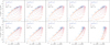 |
Fig. 5 Homogeneous warm absorber grids for HETG-MEG with typical Cyg X-1 continuum parameters for different ionization parameters logξ. Each grid is calculated for a varying equivalent hydrogen column density and covering fraction. |
4.3.1 Tracks on color–color diagrams
While the general trend of lower ionization of the absorbing material with an increasing absorption column is clear, the exact dependency of log ξ on NH is not known. We thus discuss three possible cases as shown in Fig. 6. First, building on the definition of the ionization parameter (Eq. (2)), we assume a function of the form log ξ = log(C1∕NH) for which C1 is a constant that we choose to be equal to 100 and NH in units of 1022 cm−2 (case 1). The constant C1 is chosen so that log ξ covers the range between 2.5 and 0.5 for the interesting range of NH = 0.25–32 × 1022 cm−2. Our second approach is a function of the form 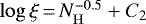 , assuming C2 to be 0 (case 2) and 0.9 (case 3), again with NH in units of 1022 cm−2. In cases 2 and 3, the ionization parameter remains higher, even at a high column density of the absorber, as would be the case in the presence of an additional ionization process, for example, collisional ionization.
We show the resulting tracks for all three cases in Fig. 7, where we also compare them to quasi-neutral absorption as calculated for logξ = −4, that is, the lowest ionization parameter accessible for the warmabs models. It can be easily seen that for cases 1 and 3, the resulting tracks show a stronger curvature, as is expected. This is not true for case 2, which closely follows the tracks of the quasi-neutral case. This can be easily understood using Fig. 6: case 2 only covers the interesting range of log ξ, where strong changes in tracks are expected (cf. Fig. 5) for small values of NH, below ~ 1022 cm−2, that is, the absorbing material is not ionized enough for ionization effects to become visible on color–color tracks.
4.3.2 Comparison to observed color–color tracks for Cyg X-1
We compare the tracks for cases 1, 2, and 3 to the Chandra observations in Fig. 8, using Γ = 1.6 and fc = 0.95 as previously mentioned. Cases 1 and 3 describe the data well. Case 2 fails to describe the curvature of the data, as is expected given that is does not cover the interesting range of the ionization parameter. We visually compare the tracks for case 1 and 3 with those obtained for constant ionization (Fig. 3, right panel): the curvature of the data is reproduced better by the two theoretical tracks with variable ionization.
This result is in agreement with our expectations of structured wind clumps with more ionized shells and less ionized cores. In such a set up, the lesser absorption episodes are then caused by either smaller clumps in our line of sight or an outer part of a larger clump crossing the line of sight, and thus we see more highly ionized material. The deepest absorption events are then caused by looking through the middle of the largest clumps, which are likely self-shielded, and they therefore exhibit lower ionization.
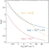 |
Fig. 6 Examples of possible dependencies of the ionization parameter, logξ, on the equivalent hydrogen absorption column density, NH, expressed in units of 1022 cm−2. |
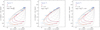 |
Fig. 7 Imhomogeneos warm absorber grids for HETG-MEG with typical Cyg X-1 continuum parameters for different dependencies of the ionization parameter logξ
on the equivalent hydrogen column density of the absorber, NH, as expressed in units of 1022 cm−2. In all cases, a grid for the quasi-neutral absorption with warmabs (logxi = −4) is shown in gray in the background to guide the eye. Left: Case 1, |
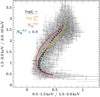 |
Fig. 8 Comparison of the color–color diagrams of the Chandra observation ObsID 3814 using the MEG M1 arm with theoretical tracks with different dependencies of the ionization parameter log ξ on the equivalent hydrogen column density; NN is expressed in units of 1022 cm−2, which is shown in solid colored lines. The dashed black line additionally shows the realization of the color–color track for a homogeneously ionized absorber with log ξ = 1.4 as presentedin the right panel of Fig. 3 and it is intended to help direct comparison. |
5 Summary and outlook
We have shown that the typical curved tracks that wind-accretion HMXBs describe on color–color diagrams during absorption events (dips) can be explained in terms of a partial covering model with variable absorption. In particular, the tracks are due to changes in the effective absorbing column density and, for reasonable assumption of a power-law-like continuum shape, they are not due to the variability of other model parameters.
For a realistic modeling of the color–color tracks, it is crucial to take into account the ionization of the absorbing wind material. Todo so, we used the warmabs family of models, with both a constant ionization parameter and an ionization parameter, which depends on the equivalent absorbing column density. The second set up can be explained as dense wind clumps embedded in tenuous, hot inter-clump material and irradiated by X-rays from the compact object.
In particular, we compare with Chandra/HETG observation of the HMXB Cyg X-1 and show that both the neutral absorber cannot explain the curvature of the tracks. A homogeneously ionized absorber with a mild ionization of log ξ ≈ 1.6 fares better.The best description is achieved if the ionization of the absorbing material is a function of the absorbing column density, specifically if the ionization decreases with an increasing column.
The approach presented here opens several avenues for further work. Color–color diagrams could be used to test whether the material causing the increase in absorption, in the cases where detailed high resolution spectroscopic analysis are not available, for example, are due to the use of CCD based instruments or due to low count rates either because of intrinsic source faintness or due to the short duration of dipping events. Further, El Mellah et al. (2020) have recently presented the theoretical framework for a formalism that, based on simulations of different line of sights through simplified clumpy winds, connects short-term absorption variability with clump size and mass. Given observationsof a sufficient length at a given orbital phase, color–color tracks could be used to obtain absorption light curves with enough time resolution to constrain absorption variability and thus to test their clumpy wind models.
Acknowledgements
V.G. is supported through the Margarete von Wrangell fellowship by the ESF and the Ministry of Science, Research and the Arts Baden-Württemberg. Work at LLNL was performed under the auspices of the U.S. Department of Energy under Contract No. DE-AC52-07NA27344 and supported by NASA grants to LLNL. M.A.N. was supported by NASA Grant NNX12AE37G in earlier stages of this work. This research has made use of NASA’s Astrophysics Data System Bibliographic Service (ADS) and of ISIS functions (isisscripts) (http://www.sternwarte.uni-erlangen.de/isis/) provided by ECAP/Remeis observatory and MIT. We in particular thank Mirjam Oertel, who developed the first versions of some of the scripts calculating the color–color tracks for arbitrary input functions, and John E. Davis for the development of the slxfig (http://www.jedsoft.org/fun/slxfig/) module used to prepare the figures in this work. We acknowledge fruitful discussions with and ideas of J. Wilms. Some of the color schemes used were based on Paul Tol’s color-blindness-friendly palettes and templates (https://personal.sron.nl/ pault/).
References
- Arnaud, K. A. 1996, ASP Conf. Ser., 101, 17 [Google Scholar]
- Bałucińska-Church, M., Church, M. J., Charles, P. A., et al. 2000, MNRAS, 311, 861 [NASA ADS] [CrossRef] [Google Scholar]
- Basak, R., Zdziarski, A. A., Parker, M., & Islam, N. 2017, MNRAS, 472, 4220 [NASA ADS] [CrossRef] [Google Scholar]
- Bautista, M. A., & Kallman, T. R. 2001, ApJS, 134, 139 [NASA ADS] [CrossRef] [Google Scholar]
- Blondin, J. M., Kallman, T. R., Fryxell, B. A., & Taam, R. E. 1990, ApJ, 356, 591 [NASA ADS] [CrossRef] [Google Scholar]
- Boroson, B., Vrtilek, S. D., Kallman, T., & Corcoran, M. 2003, ApJ, 592, 516 [NASA ADS] [CrossRef] [Google Scholar]
- Bozzo, E., Giunta, A., Cusumano, G., et al. 2011, A&A, 531, A130 [NASA ADS] [CrossRef] [EDP Sciences] [Google Scholar]
- Carpano, S., Wilms, J., Schirmer, M., & Kendziorra, E. 2005, A&A, 443, 103 [NASA ADS] [CrossRef] [EDP Sciences] [Google Scholar]
- Cohen, D. H., Gagné, M., Leutenegger, M. A., et al. 2011, MNRAS, 415, 3354 [NASA ADS] [CrossRef] [Google Scholar]
- El Mellah, I., Sundqvist, J. O., & Keppens, R. 2018, MNRAS, 475, 3240 [NASA ADS] [CrossRef] [Google Scholar]
- El Mellah, I., Grinberg, V., Sundqvist, J. O., Driessen, F. A., & Leutenegger, M. A. 2020, A&A, 643, A9 [NASA ADS] [CrossRef] [EDP Sciences] [Google Scholar]
- Feldmeier, A. 1995, A&A, 299, 523 [NASA ADS] [Google Scholar]
- Ferrigno, C., Bozzo, E., & Romano, P. 2020, A&A 642, A73 [CrossRef] [EDP Sciences] [Google Scholar]
- Fornasini, F. M., Tomsick, J. A., Bachetti, M., et al. 2017, ApJ, 841, 35 [NASA ADS] [CrossRef] [Google Scholar]
- Fullerton, A. W., Massa, D. L., & Prinja, R. K. 2006, ApJ, 637, 1025 [NASA ADS] [CrossRef] [Google Scholar]
- Fürst, F., Kreykenbohm, I., Pottschmidt, K., et al. 2010, A&A, 519, A37 [NASA ADS] [CrossRef] [EDP Sciences] [Google Scholar]
- Fürst, F., Pottschmidt, K., Wilms, J., et al. 2014, ApJ, 780, 133 [NASA ADS] [CrossRef] [Google Scholar]
- García, F., Fogantini, F. A., Chaty, S., & Combi, J. A. 2018, A&A, 618, A61 [CrossRef] [EDP Sciences] [Google Scholar]
- Grinberg, V., Hell, N., Pottschmidt, K., et al. 2013, A&A, 554, A88 [NASA ADS] [CrossRef] [EDP Sciences] [Google Scholar]
- Grinberg, V., Leutenegger, M. A., Hell, N., et al. 2015, A&A, 576, A117 [NASA ADS] [CrossRef] [EDP Sciences] [Google Scholar]
- Grinberg, V., Hell, N., El Mellah, I., et al. 2017, A&A, 608, A143 [NASA ADS] [CrossRef] [EDP Sciences] [Google Scholar]
- Haberl, F., White, N. E., & Kallman, T. R. 1989, ApJ, 343, 409 [NASA ADS] [CrossRef] [Google Scholar]
- Hanke, M. 2011, PhD thesis, Astronomisches Institut der Universität Erlangen-Nürnberg, Bamberg, Germany [Google Scholar]
- Hanke, M., Wilms, J., Nowak, M. A., et al. 2008, in Microquasars and Beyond [Google Scholar]
- Hanke, M., Wilms, J., Nowak, M. A., et al. 2009, ApJ, 690, 330 [NASA ADS] [CrossRef] [Google Scholar]
- Hemphill, P. B., Rothschild, R. E., Markowitz, A., et al. 2014, ApJ, 792, 14 [NASA ADS] [CrossRef] [Google Scholar]
- Hickox, R. C., Narayan, R., & Kallman, T. R. 2004, ApJ, 614, 881 [NASA ADS] [CrossRef] [Google Scholar]
- Hirsch, M., Hell, N., Grinberg, V., et al. 2019, A&A, 626, A64 [NASA ADS] [CrossRef] [EDP Sciences] [Google Scholar]
- Houck, J. C. 2002, ARA&A, 41, 291 [Google Scholar]
- Houck, J. C., & Denicola, L. A. 2000, ASP Conf. Ser., 216, 591 [Google Scholar]
- Kallman, T., & Bautista, M. 2001, ApJS, 133, 221 [NASA ADS] [CrossRef] [Google Scholar]
- Kallman, T. R., Bautista, M. A., Goriely, S., et al. 2009, ApJ, 701, 865 [NASA ADS] [CrossRef] [Google Scholar]
- Li, F. K., & Clark, G. W. 1974, ApJ, 191, L27 [NASA ADS] [CrossRef] [Google Scholar]
- Lomaeva, M., Grinberg, V., Guainazzi, M., et al. 2020, A&A, 641, A144 [NASA ADS] [CrossRef] [EDP Sciences] [Google Scholar]
- Martínez-Núñez, S., Torrejón, J. M., Kühnel, M., et al. 2014, A&A, 563, A70 [NASA ADS] [CrossRef] [EDP Sciences] [Google Scholar]
- Martínez-Núñez, S., Kretschmar, P., Bozzo, E., et al. 2017, Space Sci. Rev., 212, 59 [NASA ADS] [CrossRef] [Google Scholar]
- Miškovičová, I., Hell, N., Hanke, M., et al. 2016, A&A, 590, A114 [NASA ADS] [CrossRef] [EDP Sciences] [Google Scholar]
- Naik, S., Paul,B., & Ali, Z. 2011, ApJ, 737, 79 [NASA ADS] [CrossRef] [Google Scholar]
- Noble, M. S., & Nowak, M. A. 2008, PASP, 120, 821 [NASA ADS] [CrossRef] [Google Scholar]
- Nowak, M. A., Hanke, M., Trowbridge, S. N., et al. 2011, ApJ, 728, 13 [NASA ADS] [CrossRef] [Google Scholar]
- Odaka, H., Khangulyan, D., Tanaka, Y. T., et al. 2013, ApJ, 767, 70 [NASA ADS] [CrossRef] [Google Scholar]
- Oskinova, L. M., Feldmeier, A., & Kretschmar, P. 2012, MNRAS, 421, 2820 [NASA ADS] [CrossRef] [Google Scholar]
- Owocki, S. P., & Rybicki, G. B. 1984, ApJ, 284, 337 [NASA ADS] [CrossRef] [Google Scholar]
- Sander, A. A. C., Fürst, F., Kretschmar, P., et al. 2018, A&A, 610, A60 [NASA ADS] [CrossRef] [EDP Sciences] [Google Scholar]
- Skipper, C. J., McHardy, I. M., & Maccarone, T. J. 2013, MNRAS, 434, 574 [NASA ADS] [CrossRef] [Google Scholar]
- Sundqvist, J. O., & Owocki, S. P. 2013, MNRAS, 428, 1837 [NASA ADS] [CrossRef] [Google Scholar]
- Sundqvist, J. O., Owocki, S. P., & Puls, J. 2018, A&A, 611, A17 [NASA ADS] [CrossRef] [EDP Sciences] [Google Scholar]
- Tarter, C. B., Tucker, W. H., & Salpeter, E. E. 1969, ApJ, 156, 943 [NASA ADS] [CrossRef] [Google Scholar]
- Torrejón, J. M., Schulz, N. S., Nowak, M. A., et al. 2015, ApJ, 810, 102 [NASA ADS] [CrossRef] [Google Scholar]
- Verner, D. A., Ferland, G. J., Korista, K. T., & Yakovlev, D. G. 1996, ApJ, 465, 487 [Google Scholar]
- Wilms, J., Allen, A., & McCray, R. 2000, ApJ, 542, 914 [Google Scholar]
- Xu, Y., McCray, R., & Kelley, R. 1986, Nature, 319, 652 [Google Scholar]
- Yamada, S., Torii, S., Mineshige, S., et al. 2013, ApJ, 767, L35 [Google Scholar]
This model was formerly known as tbnew and since 2016 has been included as the default tbabs version in xspec Arnaud (1996); it is thus also the default tbabs version in all packages that rely on xspec models, such as ISIS.
All Figures
|
Fig. 1 Principle demonstration of the effect of a variable partial covering absorption on an absorbed powerlaw with photon index Γ = 1.7 and ISM absorption |
| In the text | |
|
Fig. 2 Simulated color–color tracks for varying parameters of a partially absorbed power law model for HETG-MEG and parameter ranges typical for the HMXB Cygnus X-1. |
| In the text | |
|
Fig. 3 Comparison of the color–color diagrams of the Chandra observation ObsID 3814 using the MEG M1 arm with different models. Left: empirical polynomial fit. Middle: neutral grid using the tbabs absorption model for different covering fractions and the same continuum photon index Γ = 1.6. Right: homogeneously ionized absorber using the warmabs model with continuum photon index Γ = 1.6 and a covering fraction of 0.95. The equivalent absorbing column density,NH, changes from 0.25 × 10⁻²² cm−2 to 32 × 10−22 cm−2 along each line, with each line showing the track for a different ionization parameter log ξ as indicated by the different colors. |
| In the text | |
|
Fig. 4 Relative transmission in the 0.5–10 keV band for an equivalent hydrogen column density of NH = 2 × 1022 cm−2 and varyingionization parameters using warmabs shown in color. For comparison, neutral absorption as modeled with the tbabs model for the same hydrogen column density is shown in gray. |
| In the text | |
|
Fig. 5 Homogeneous warm absorber grids for HETG-MEG with typical Cyg X-1 continuum parameters for different ionization parameters logξ. Each grid is calculated for a varying equivalent hydrogen column density and covering fraction. |
| In the text | |
|
Fig. 6 Examples of possible dependencies of the ionization parameter, logξ, on the equivalent hydrogen absorption column density, NH, expressed in units of 1022 cm−2. |
| In the text | |
|
Fig. 7 Imhomogeneos warm absorber grids for HETG-MEG with typical Cyg X-1 continuum parameters for different dependencies of the ionization parameter logξ
on the equivalent hydrogen column density of the absorber, NH, as expressed in units of 1022 cm−2. In all cases, a grid for the quasi-neutral absorption with warmabs (logxi = −4) is shown in gray in the background to guide the eye. Left: Case 1, |
| In the text | |
|
Fig. 8 Comparison of the color–color diagrams of the Chandra observation ObsID 3814 using the MEG M1 arm with theoretical tracks with different dependencies of the ionization parameter log ξ on the equivalent hydrogen column density; NN is expressed in units of 1022 cm−2, which is shown in solid colored lines. The dashed black line additionally shows the realization of the color–color track for a homogeneously ionized absorber with log ξ = 1.4 as presentedin the right panel of Fig. 3 and it is intended to help direct comparison. |
| In the text | |
Current usage metrics show cumulative count of Article Views (full-text article views including HTML views, PDF and ePub downloads, according to the available data) and Abstracts Views on Vision4Press platform.
Data correspond to usage on the plateform after 2015. The current usage metrics is available 48-96 hours after online publication and is updated daily on week days.
Initial download of the metrics may take a while.