| Issue |
A&A
Volume 643, November 2020
|
|
|---|---|---|
| Article Number | C1 | |
| Number of page(s) | 2 | |
| Section | Letters to the Editor | |
| DOI | https://doi.org/10.1051/0004-6361/201834222e | |
| Published online | 09 November 2020 | |
Letter to the Editor
Synchrotron emission in molecular cloud cores: the SKA view (Corrigendum)
INAF–Osservatorio Astrofisico di Arcetri, Largo E. Fermi 5, 50125 Firenze, Italy
e-mail: This email address is being protected from spambots. You need JavaScript enabled to view it.
, This email address is being protected from spambots. You need JavaScript enabled to view it.
Key words: ISM: clouds / ISM: magnetic fields / cosmic rays / errata / addenda
The specific intensity (Eq. (5)) has not been correctly evaluated1. This affects the computation of the flux densities, whose correct trends are shown in the new versions of Figs. 3 and 4. We recovered the signal-to-noise ratios (S/Ns) quoted in the paper by assuming a magnetic field strength B0 larger by a factor of 2.74 − 4.20, 2.02 − 2.72, and 1.55 − 1.80 than originally assumed for models A, B, and C, respectively (the lower and upper values corresponding to κ = 0.5 and κ = 0.7, respectively). The conclusions of the paper are unaffected.
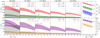 |
Fig. 3. Radial flux density profiles for the starless core models described in Sect. 5.1 (upper row) and for B68 and FeSt 1-457 (lower row, see Sect. 5.2). The observing frequency is shown in black at the top of each column, while numbers in the upper-right corner of each subplot represent the radius-averaged S/N for the two values of κ (0.5 and 0.7 for models A, B, C, and B68, and 0.68 and 0.88 for FeSt 1-457, see Eq. (9)). Shaded areas encompass the curves obtained with Eq. (9) by using the two values of κ (see Fig. 2 for colour-coding). The telescope beam is shown in the leftmost column for models A, B, and C (dotted black line, 300″), B68 (short-dashed black line, 330″), and FeSt 1-457 (long-dashed black line, 284″). Hatched areas display SKA sensitivities for one hour of integration at different frequencies. The two panels on the right side show the flux density as a function of frequency. Empty (solid) circles refer to an S/N smaller (larger) than 3, respectively. The spectral index α is shown on the right of each curve. |
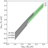 |
Fig. 4. Flux density at 60, 114, and 218 MHz (lower-left labels) as a function of magnetic field strength B0 for model B (see Sect. 5.1). Green shaded areas encompass the curves obtained with Eq. (9) by using κ = 0.5 and 0.7. Grey areas correspond to an S/N < 3 and dashed lines are power-law fits of |

We thank Alexei Ivlev for pointing out this mistake.
© ESO 2020
All Figures
|
Fig. 3. Radial flux density profiles for the starless core models described in Sect. 5.1 (upper row) and for B68 and FeSt 1-457 (lower row, see Sect. 5.2). The observing frequency is shown in black at the top of each column, while numbers in the upper-right corner of each subplot represent the radius-averaged S/N for the two values of κ (0.5 and 0.7 for models A, B, C, and B68, and 0.68 and 0.88 for FeSt 1-457, see Eq. (9)). Shaded areas encompass the curves obtained with Eq. (9) by using the two values of κ (see Fig. 2 for colour-coding). The telescope beam is shown in the leftmost column for models A, B, and C (dotted black line, 300″), B68 (short-dashed black line, 330″), and FeSt 1-457 (long-dashed black line, 284″). Hatched areas display SKA sensitivities for one hour of integration at different frequencies. The two panels on the right side show the flux density as a function of frequency. Empty (solid) circles refer to an S/N smaller (larger) than 3, respectively. The spectral index α is shown on the right of each curve. |
| In the text | |
|
Fig. 4. Flux density at 60, 114, and 218 MHz (lower-left labels) as a function of magnetic field strength B0 for model B (see Sect. 5.1). Green shaded areas encompass the curves obtained with Eq. (9) by using κ = 0.5 and 0.7. Grey areas correspond to an S/N < 3 and dashed lines are power-law fits of |
| In the text | |
Current usage metrics show cumulative count of Article Views (full-text article views including HTML views, PDF and ePub downloads, according to the available data) and Abstracts Views on Vision4Press platform.
Data correspond to usage on the plateform after 2015. The current usage metrics is available 48-96 hours after online publication and is updated daily on week days.
Initial download of the metrics may take a while.