| Issue |
A&A
Volume 642, October 2020
|
|
|---|---|---|
| Article Number | A109 | |
| Number of page(s) | 12 | |
| Section | The Sun and the Heliosphere | |
| DOI | https://doi.org/10.1051/0004-6361/202038832 | |
| Published online | 09 October 2020 | |
When do solar erupting hot magnetic flux ropes form?⋆
1
Physics Department, University of Ioannina, Ioannina 45110, Greece
e-mail: This email address is being protected from spambots. You need JavaScript enabled to view it.
2
The Johns Hopkins University Applied Physics Laboratory, Laurel, MD 20723, USA
3
School of Astronomy and Space Science, Nanjing University, Nanjing 210093, PR China
4
Max Planck Institute for Solar System Research, Göttingen 37077, Germany
5
Department of Physics and Astronomy, George Mason University, Fairfax, VA 22030, USA
Received:
3
July
2020
Accepted:
4
August
2020
Abstract
Aims. We investigate the formation times of eruptive magnetic flux ropes relative to the onset of solar eruptions, which is important for constraining models of coronal mass ejection (CME) initiation.
Methods. We inspected uninterrupted sequences of 131 Å images that spanned more than eight hours and were obtained by the Atmospheric Imaging Assembly on board the Solar Dynamics Observatory to identify the formation times of hot flux ropes that erupted in CMEs from locations close to the limb. The appearance of the flux ropes as well as their evolution toward eruptions were determined using morphological criteria.
Results. Two-thirds (20/30) of the flux ropes were formed well before the onset of the eruption (from 51 min to more than eight hours), and their formation was associated with the occurrence of a confined flare. We also found four events with preexisting hot flux ropes whose formations occurred a matter of minutes (from three to 39) prior to the eruptions without any association with distinct confined flare activity. Six flux ropes were formed once the eruptions were underway. However, in three of them, prominence material could be seen in 131 Å images, which may indicate the presence of preexisting flux ropes that were not hot. The formation patterns of the last three groups of hot flux ropes did not show significant differences. For the whole population of events, the mean and median values of the time difference between the onset of the eruptive flare and the appearance of the hot flux rope were 151 and 98 min, respectively.
Conclusions. Our results provide, on average, indirect support for CME models that involve preexisting flux ropes; on the other hand, for a third of the events, models in which the ejected flux rope is formed during the eruption appear more appropriate.
Key words: Sun: coronal mass ejections (CMEs) / Sun: flares
Movies attached to Figs. 2, 5, 8, and 10 are available at http://www.aanda.org
© ESO 2020
1. Introduction
Coronal mass ejections (CMEs) are the most spectacular form of dynamic phenomena in the solar atmosphere. They are defined as large-scale expulsions (on the order of ∼1014 to ∼1016 g) of coronal magnetized plasma into the heliosphere at speeds ranging from about 100 km s−1 to more than 2000 km s−1 (e.g., see Yashiro et al. 2004; Chen 2011, and references therein).
The preeruptive configuration of CMEs has been extensively debated. There is a vast literature on the subject, for example reviews by Forbes (2000), Klimchuk et al. (2001), Chen (2011), Aulanier et al. (2014), Schmieder et al. (2015), Cheng et al. (2017), Green et al. (2018), Georgoulis et al. (2019), and references therein. Briefly, there are two groups of CME models depending on the configuration of the coronal magnetic field before eruption. One group of models rely on the existence of a magnetic flux rope (i.e., a twisted flux tube whose magnetic field lines wind about an axial magnetic field line in the interior of the tube) prior to the eruption (e.g., Forbes & Isenberg 1991; Isenberg et al. 1993; Forbes & Priest 1995; Gibson & Low 1998; Roussev et al. 2003; Amari et al. 2004, 2005; Török & Kliem 2005; Kliem & Török 2006; Fan & Gibson 2007; Archontis & Török 2008; Archontis & Hood 2012). The most convincing observational evidence in favor of models with preexisting flux ropes is the identification of a flux-rope-like structure that is present well before the eruption (references are provided later in this section, in conjunction with the discussion of proxies to active region flux ropes).
In the models of the second group, the preeruptive configuration consists of sheared magnetic arcades, that is to say a set of arc-like magnetic field lines whose orientation deviates from the local normal to the polarity inversion line. It has been suggested that magnetic reconnection between two sheared sets of loops within the core field of a bipolar active region may create (or grow) a flux rope that immediately erupts outward (“tether-cutting” scenario, e.g., Mikić & Linker 1994; Amari et al. 1996; Roussev et al. 2004; Jacobs et al. 2006). Several eruptive events have been interpreted in terms of this model (e.g., Moore et al. 2001; Liu et al. 2012; Chen et al. 2014b, 2016; Xue et al. 2017); usually the observations include flare brightenings and weak precursor activity that takes place prior to the eruption at the core of the active region. Alternatively, the core of a sheared arcade may expand (for example, due to shearing motions) and then erupt after it breaks through the overlying magnetic field via reconnection at a null point (breakout model, see Antiochos et al. 1999; MacNeice et al. 2004; Lynch et al. 2008; Karpen et al. 2012; Lynch & Edmondson 2013). Observations favoring the breakout model include eruptions occurring in multipolar magnetic configurations (Aulanier et al. 2000; Ugarte-Urra et al. 2007) as well as small-scale brightenings that appear away from the active region core (e.g., see Sterling & Moore 2004 and references therein).
Although there is no broad consensus on the state of the preeruptive magnetic field, practically all models predict that the CME will contain a flux rope after eruption; in other words, while the flux rope is an integral part of the preeruptive configuration in the first group of models, it forms during the eruption in the second group of models. Therefore, it is important to know when the flux rope that subsequently erupts is formed.
Since the ejected structure is a flux rope, white light coronagraph observations of CMEs or in situ solar wind measurements cannot provide a direct way to determine the type of preeruptive configuration. Searching for evidence for the existence of preeruptive flux ropes in the low corona is complicated by the lack of routine observations of the coronal magnetic field. Therefore, we usually resort to proxies. In active regions, the following four proxies have been used: (1) thread orientation in filaments (e.g., López Ariste et al. 2006; Jiang et al. 2014; Yardley et al. 2016; Chandra et al. 2017; Xue et al. 2016); (2) soft X-ray sigmoids when their middle section crosses the polarity inversion line in the inverse direction (e.g., Green & Kliem 2009; Green et al. 2011) and when their ends turn around to point toward the center of the S; (3) nonlinear force-free field (NLFFF) extrapolations of the photospheric vector magnetograms (e.g., Yan et al. 2001; Canou et al. 2009; Guo et al. 2013; Chintzoglou et al. 2015; Amari et al. 2018; James et al. 2018; Duan et al. 2019); and (4) hot flux ropes. Regarding this last proxy, high-cadence, high spatial resolution observations obtained with the Atmospheric Imaging Assembly (AIA; Lemen et al. 2012) aboard the Solar Dynamics Observatory (SDO; Pesnell et al. 2012) have revealed the existence of coherent “hot channels” or “hot blobs” (Reeves & Golub 2011; Cheng et al. 2011, 2012, 2013, 2014a,b,c; Zhang et al. 2012; Li & Zhang 2013; Tripathi et al. 2013; Patsourakos et al. 2013; Chen et al. 2014a, 2020; Joshi et al. 2014; Song et al. 2014; Vemareddy & Zhang 2014; Nindos et al. 2015; Chintzoglou et al. 2015; James et al. 2017, 2018; Zhou et al. 2017; Veronig et al. 2018; Wang et al. 2019). These structures appear in the 131 Å passband, which probes temperatures of ∼10 MK during flares, but they do not appear in cooler passbands that probe quiescent coronal temperatures (≲2 MK).
These hot channels and blobs have been identified as hot flux ropes based on morphological criteria (see Sect. 2), which interpret observations on the grounds of theoretical expectations. Obviously, this interpretation of observations may have to be modified in the future if needed. Therefore, it would probably be more appropriate to use the term “candidate hot flux ropes” but for the sake of brevity we will, instead, adopt the term “hot flux ropes” (HFRs) throughout the paper.
The appearance of HFRs is quite common in large events; using an extensive dataset of 141 M-class and X-class flares that occurred relatively close to the limb, Nindos et al. (2015; hereafter referred to as Paper I) found HFRs in 45 of them (32%). Furthermore, they detected HFRs in 34 of their 70 eruptive events (49%).
There are several case studies on the formation times of HFRs. These studies take advantage of the high-cadence uninterrupted sequence of full-disk observations provided by the AIA and are also favored by the fact that the candidate flux ropes usually remain coherent throughout most of their evolution. A few events with HFRs forming during the eruption have been reported (e.g., Cheng et al. 2011; Song et al. 2014; Veronig et al. 2018). Most publications report preexisting HFRs, but the times of the reported appearances are biased by the duration of the observational window. Those that use rather short observational windows around the eruption report the formation of HFRs a matter of minutes (two to 30) before the onset of the eruption (Cheng et al. 2013; Li & Zhang 2013; Tripathi et al. 2013; Cheng et al. 2014a,c; Vemareddy & Zhang 2014; Cheng et al. 2015).
Patsourakos et al. (2013) were the first to report the formation of an HFR well before its eruption (about seven hours), during a confined flare. If they had used a shorter time interval they would have missed the confined event and their conclusion about the time of the HFR formation would have been different. In subsequent publications, similar conclusions about the formation of HFRs long before the eruption (from one to more than 11 hours) were reported by a number of authors (Chen et al. 2014a; Cheng et al. 2014b; Chintzoglou et al. 2015; James et al. 2017, 2018; Kumar et al. 2017; Zhou et al. 2017; Liu et al. 2018; Wang et al. 2019).
The above publications were case studies that did not address the statistics of the formation times of HFRs in eruptive events. With the present study, we aim to remedy this issue by determining the formation times of HFRs in an extensive dataset of large eruptive events using observations that cover several hours before the onset of the eruptions. The paper is organized as follows. In Sect. 2, we present the observations and data analysis. In Sect. 3, we introduce our classification of events in terms of the formation times of the HFRs. In Sect. 4, we discuss each category of events. Finally, in Sect. 5, we discuss our results and conclude.
2. Observations and data analysis
Our starting point was the 34 eruptive M-class and X-class flare events from Paper I that involved an HFR configuration. We analyzed each event using extreme ultra-violet (EUV) images of the low corona from the AIA. The pixel size, cadence, and field of view of the AIA images are 0.6″, 12 s, and 1.3 R⊙, respectively. We used images obtained in narrowband channels centered at 94, 131, 171, 193, 211, 304, and 335 Å, which have peak responses at about 6.3, 10, 0.6, 1.6, 2.0, 0.05, and 2.5 × 10⁶ K, respectively (Lemen et al. 2012). The emission in the 94 and 131 Å passbands probes multi-million Kelvin plasma only during flares; during quiescent periods, their signal is dominated by emissions from cooler plasmas with temperatures below 106 K (O’Dwyer et al. 2010). In each passband, our data covered an interval of more than eight hours, ending a few minutes after the onset time of the eruption. The study of time intervals much longer than those in Paper I (the maximum duration of the movies we used in Paper I was one hour) was deemed necessary for the identification of HFRs that formed long before the eruptions.
To reduce data size, the cadence of the AIA data was degraded to two minutes. For selected events, we compared movies made with two-minute cadences with full-cadence movies and found that the two-minute cadence was adequate to capture the various dynamics. All images of each event were rotated to a common reference time to correct for solar rotation.
In Paper I, the identification of the flux ropes was done using 131 Å data obtained around the time of the eruptive flares and employing a set of morphological criteria. Briefly, these included the identification of: (1) ring-like structures or round blobs interpreted as flux ropes seen edge-on. These structures usually appeared on top of Λ-shaped features, cusps, and current-sheet-like thin elongated features. (2) Tangled threads winding around a central, axial direction or either twisted or writhed structures interpreted as flux ropes seen face-on. Close to disk center, sigmoidal structures were also interpreted as flux ropes seen face-on. (3) Configurations with coexisting morphologies of both cases (1) and (2) interpreted as flux ropes seen from intermediate viewpoints.
The same criteria were also used for the identification of and for monitoring the evolution of the flux ropes in our eight-hour-long 131 Å movies. As in Paper I, we ensured that all candidate flux ropes were hot by their absence in the 171 and 304 Å movies.
In Paper I, the existence of HFRs in 131 Å was further confirmed by the identification of flux rope structures in Hinode X-ray Telescope (XRT) data. The response of all XRT filters is broad (see Narukage et al. 2011), which allows them to probe material at a broad temperature range (from above 2 MK to more than 10 MK for the thin filters). Therefore, as we noted in Paper I, looking at thin-filter XRT images can be considered as roughly equivalent to looking at images from the narrowband 211, 335, and 94 Å AIA passbands. However, only ten of the 34 eruptive AIA events were also observed by the XRT, and flux rope morphologies were detected in seven of them. Furthermore, it was difficult to find uninterrupted eight-hour-long sequences of XRT data for any of them. For these reasons, instead of checking XRT data for the long-term evolution of flux ropes, we checked eight-hour-long sequences of images from 94, 193, 211, and 335 Å AIA passbands for this paper. All HFRs identified in the 131 Å data appear in 94 Å as well, but only 12 of them appear in some of the cooler passbands centered at 211 and 335 Å (and these appear fuzzier and for limited time intervals). In agreement with the results of Paper I, none of them appeared in the eight-hour-long movies of the coolest passbands centered at 171 and 304 Å.
Inspired by the work of Patsourakos et al. (2013), who reported the formation of an HFR during a confined flare several hours before the eruption of the flux rope, we searched for confined flares associated with the appearance of the HFRs that later erupted. As will be seen in Sect. 3, that correlation (or the absence thereof) was an important ingredient of the classification scheme that we adopted. To this end, for each event we constructed light curves in all AIA channels that we used by integrating the emission (normalized to unity exposure time) within a box containing the HFR after its appearance.
3. Classification of events
The first and last milestones in the evolution of an eruptive flux rope in the low corona are the time of its appearance and the time of its eruption, respectively. The appearance times of the HFRs were determined using the morphological criteria outlined in Sect. 2 (see also Paper I). We note that an uncertainty of one minute in the determination of the formation times of the HFRs is introduced by the cadence of the datasets we used. However, this should be considered as a lower limit; in fact, an uncertainty greater than the nominal 1 minute should be present due to the ambiguities involved in determining the appearance of the HFRs in the 131 Å data; this was done visually and is inevitably subjective.
An accurate determination of the onset time of an eruption would require the construction of a height-time plot computed along the central direction of the ejection as well as its subsequent fitting with some function; this could capture the kinematic phases of the erupting flux rope (e.g., see Zhang et al. 2012; Cheng et al. 2013, 2014a, 2020) and, particularly, the break point, which indicates the onset time of the main acceleration phase of the eruption. We did not follow that approach because of the large size of our dataset and the complexity of the relevant calculations (see the discussion in Cheng et al. 2020). We also did not use results from the backward extrapolation of white-light CME height-time plots because they do not reflect the early evolution of the event. Instead, we used the onset time of the eruptive flare as a reasonable proxy for the onset time of the eruption. Following Cheng et al. (2020), we found the onset time of the eruptive flares by inspecting the GOES 1–8 Å flux time profiles and determining the time beginning from which the flux increases monotonically and far more rapidly than before. In 30 out of the 34 events, our estimates agreed with the flare onset times provided by the GOES flare list1, while in the remaining cases the differences were less than 5 min. Cheng et al. (2020) find differences between the onset time of the flux rope’s acceleration phase and the onset of the eruptive flare that ranged from −4 to 2 min for the six active region 131 Å hot channel structures they studied. Therefore, our approach may introduce an uncertainty of about 3–4 min in the determination of the onset time of the eruption.
Overall, the HFR was formed during the eruption in six events and appeared before the eruption in 28 events (we note that in four out of the 28, the formation time was ambiguous). However, this simple grouping does not provide much insight into the situation. We refined our classification by considering whether or not the appearance of the HFR was associated with the occurrence of a confined flare. We define an enhancement in the 131 or 94 Å light curves with the following properties as a “confined flare” : (i) its maximum intensity is above the 1.5σ level of the background emission, and (ii) it drops below half its peak before the onset of the eruptive flare.
The choice of the σ multiplication factor used in our definition of confined flares certainly affects the results. Our experience with the data shows that a threshold at about 2σ or higher would miss a few cases with conspicuous brightenings in the hot AIA passbands, while a threshold lower than 1.5σ would tend to include weak transient activity (e.g., Shimizu 1995; Hannah et al. 2008), which is ubiquitous in active regions. With our second criterion for the definition of confined flares, we excluded precursor brightenings that occurred in close temporal proximity with large eruptive flares.
According to our refined scheme, we classified our events into the following five categories. First are HFR events that are formed on the fly during the eruption with no evidence of prominence material in the 131 Å images (FLY in Table 1). The HFR appears at or after the onset of the eruptive flare. Examples are presented in Figs. 1–3. The second category is the same as the first group but prominence material can be identified in 131 Å images (FLYP in Table 1). An example is presented in Fig. 1. Third are events with HFRs that are formed before the onset of the eruptive flare but whose formations are not associated with any distinct confined flares (PRE in Table 1). Examples are presented in Figs. 4– 6. The fourth category is the same as the third group, but the formation is associated with a confined flare (PREC in Table 1). Examples are presented in Figs. 7– 11. Fifth is uncertain events in which the flux rope is most probably formed before the eruption and where there is ambiguity in the determination of its appearance; this is primarily because more than one appear during the eight-hour interval and it is unclear which one finally erupts (UNC in Table 1).
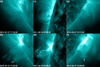 |
Fig. 1. Events, at 131 Å, with HFRs formed during the eruption with (middle and right-hand columns; FLYP) and without (left column; FLY) preexisting prominence material. Top row: snapshots of the pre-event configuration. Bottom row: snapshots after the appearance of the HFRs. The images of the left-hand, middle, and right-hand columns correspond to events 70, 5, and 99 in Table 1, respectively. The arrows mark the HFRs. The field of view in each image is 300 × 300 arcsec2. |
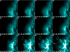 |
Fig. 2. Example of the formation, at 131 Å, of an HFR during the eruption (FLY; event 89 in Table 1). The arrows mark the HFR. The box in panel j marks the area used for the calculations presented in Fig. 3. The field of view is 300 × 300 arcsec2. See also the associated online movie. |
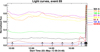 |
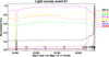
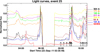
Fig. 3. Light curves in 94, 131, 171, 193, 211, 304, and 335 Å AIA passbands from the region marked with the box shown in Fig. 2j as well as in the GOES 1–8 Å channel. All curves are normalized to their maximum values. The vertical dashed line marks the first appearance of the HFR. The arrows just above the horizontal axis mark the times of the images displayed in Fig. 2. |
Timing of HFR eruptive events.
In ten regions that produced events very close to the limb, we detected partially occulted confined flares during parts of the eight-hour-long intervals that we used. However, post-flare loops were readily visible beyond the limb in all cases. In the hot 94 and 131 Å passbands, the emission from post-flare loop arcades is usually higher than the footpoint emission; therefore, it is rather unlikely that we missed, due to partial occultation, the registration of any significant confined flare activity in the 94 or 131 Å light curves. Furthermore, since flux ropes correspond to presumably longer magnetic field lines that expand above post-flare loops, we are confident that we did not miss any early formation of flux ropes associated with occulted confined flares.
Our classification is presented in Table 1. The first three columns (from left to right) show the event number as was registered in Paper I, the start and peak times of the eruptive flare, and the time of appearance of the HFR. In the fourth column we give the time difference, Δt, between the onset of the eruptive flare and the appearance of the HFR. In the fifth column we provide information about the possible occurrence of a confined flare associated with the appearance of the HFR. In parentheses we give the maximum value of the 131 Å confined flare emission in million data numbers per second (DN s−1) and, when there was also trace of the flare in GOES 1–8 Å flux time profiles, its strength according to its GOES classification. We note that we consider the 131 Å values more reliable due to the higher sensitivity of the AIA and because the GOES light curves record full-disk fluxes. Events for which the confined flare was detected only in the AIA data are marked with an asterisk. In the sixth column we give the classification of the events into five categories.
4. Formation patterns of eruptive hot flux ropes
4.1. Hot flux ropes formed during eruption
In the left-hand column of Fig. 1, we present an example of a FLY event, while in the middle and right-hand columns we present examples of FLYP events. In the bottom row of the figure, we show the three HFRs that are formed during the eruption. The flare brightenings are prominent in all three bottom panels, while the HFRs are marked with arrows. In panel d, the HFR appears as a rounded arc coexisting with some prominence material; there is also a thin elongated current-sheet-like structure underneath the flux rope. In panel b, the HFR appears as an elliptical blob that sits on a Λ-shaped loop-like structure, while in panel f its presence is reflected by the twisted shape of the loops. In the same figure, the corresponding top panels show characteristic snapshots of the preeruptive configuration a few minutes before the onset of the eruption. No conspicuous trace of HFRs or of brightenings associated with their appearances can be detected in the pre-event images, and that was the case throughout the eight-hour-long intervals that we checked. However, prominence material can be seen in both panels c and e, which could indicate the presence of preexisting flux ropes (if we assume that prominence plasma can be found in flux rope segments), which are not hot due to insufficient heating through magnetic reconnection.
A more detailed presentation of a FLY event (event 89 of Table 1) is given in Fig. 2 (see also the associated movie). Panels a–g show selected snapshots of the evolution of the pre-event configuration in 131 Å. The active region consists of semi-circular loops, which are not static; no major restructuring takes place for more than 9.5 hours, although weak transient brightenings can occasionally be detected. Starting at 17:24 UT (panel h), bright sheared loops appear intermingled with lower-lying prominence-like material. These loops rise, grow, and tangle along their spine as shown in panel i, which probably marks the time of appearance of the HFR. Around the same time, the core of the active region flares up. Panels j and k show the full development of the rising HFR, while in panel l the HFR is marginally detectable due to its proximity to the edge of the field of view.
Panels j–l show that the HFR ejection occurs simultaneously with the eruptive flare. This is also shown in the light curves of Fig. 3, which have been computed from the region enclosed by the box of Fig. 2, panel j. In Fig. 3, the vertical dashed line marks the appearance of the HFR. We note the precursor local peak in the 94 Å light curve about 30 min before the appearance of the HFR. That local peak is related to a diffuse transient low-lying enhancement, which is marginally visible at 131 Å, just above the limb in Fig. 2, panel f. In any case, according to our criteria (see Sect. 3), it does not qualify as a confined flare because its emission has not dropped below its half maximum value at the onset time of the eruptive flare.
4.2. Preexisting hot flux ropes without confined flares
Snapshots of two events with preexisting HFRs whose formations were not associated with the occurrence of confined flares (PRE events) are presented in Fig. 4. For both events, the top row corresponds to the early development of the HFRs, while the images of the bottom row were obtained at a later stage. In both events, the formation of the HFRs is not associated with any confined flaring activity, as was defined in Sect. 3. In the event presented in the left-hand column, the HFR appears as a twisted structure relatively high above the limb (uncorrected height of about 180″, see panel a). Sixteen minutes later, in panel b, the HFR has moved outward and its size has increased, while lower down bright flaring loops have appeared. In the event presented in the right-hand column, the HFR appears as a round blob four minutes before the onset of the eruptive flare (see panel c for a characteristic snapshot of its early development). Panel d shows that six minutes later the HFR has grown, moving in the southeast direction while the eruptive flare is in progress.
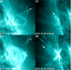 |
Fig. 4. Events, at 131 Å, with preexisting HFRs whose formations were not associated with confined flares (PRE). Top row: snapshots of HFRs observed a few minutes after their appearance. Bottom row: the flux ropes of the top row observed at a later stage. The images of the left- and right-hand columns correspond to events 35 and 107 in Table 1, respectively. The arrows mark the HFRs. The field of view in each image is 300 × 300 arcsec2. |
In Fig. 5 (see also the associated online movie), we give a more detailed presentation of a PRE event (event 61 of Table 1). Panels a–d show selected snapshots from the preeruptive configuration, which show no evidence of the presence of a flux-rope-like structure (see also the movie). From about 00:34 onward (see panel e for an example), the structure of the active region changes because of the development of undulatory loops, which grow and gradually develop tangled threads and twisted tips that probably both reflect the appearance of the HFR (panel f). Some of the twisted tips merge to form a round blob that sits on top of a Λ-shaped system of loops (see panels f to i). The development and outward motion of that feature can be tracked in panels j–k, while at the same interval the eruptive flare is in progress. In panel l, the HFR has left the field of view of the instrument.
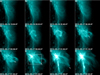 |
Fig. 5. Example of the evolution, at 131 Å, of a preexisting HFR whose formation was not associated with a confined flare (PRE; event 61 in Table 1). The arrows mark the HFR. The box in panel j marks the area used for the calculations presented in Fig. 6. The field of view is 300 × 300 arcsec2. See also the associated online movie. |
The light curves of Fig. 6 have been computed from the region inside the box of Fig. 5, panel j. Both the 131 Å and 94 Å (and to some extent the 335 Å) light curves show enhancements that start around the time of appearance of the HFR and are practically indistinguishable from the main eruptive flare.
4.3. Preexisting hot flux ropes with confined flares
In the events with preexisting HFRs that were formed in conjunction with confined flares (PREC events), the flare appeared in most AIA passbands that we studied, and occasionally in the X-ray fluxes recorded by GOES. The confined nature of the flares was judged by the absence of large-scale EUV dimmings in the AIA data and the absence of white-light CMEs in the Large Angle Spectroscopic Coronagraph (LASCO; Brueckner et al. 1995) data.
In Fig. 7, we present snapshots of three PREC events. The top row shows the HFRs a few minutes after their appearance, while the bottom row shows them in the course of the eruption. The HFRs of the left-hand, middle, and right-hand columns (events 81, 97, and 133 of Table 1) appeared 197, 86, and 451 min, respectively, before the onset of the eruptive flare. At the early stage of their development, the HFRs of events 81 and 97 (see panels a and c) show ring-like structures (we note that the flux-rope-like feature south of the HFR marked with the arrow in panel a did not participate in the eruption) that sit on top of thin elongated current-sheet-like structures, and this shows better for event 81. On the other hand, panel e indicates that the HFR of event 133 appears as a round blob that sits on top of a Λ-shaped loop. Although the time interval between the images of panels a and b is 190 min, the HFR morphology and size has not changed significantly. However, panels d and f show that the HFRs of events 97 and 133 have grown considerably in the course of their evolution; in addition to its growth, the south part of the initial ring-like structure has deformed in event 97.
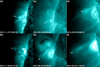 |
Fig. 7. Same as Fig. 4 but for preexisting HFRs whose formations were associated with confined flares (PREC). The images in the left-hand, middle, and right-hand columns correspond to events 81, 97, and 133 in Table 1, respectively. The field of view in each image is 300 × 300 arcsec2 except in those of the middle column where it is 360 × 360 arcsec2. |
In Fig. 8, we present the evolution of a PREC event (event 25 of Table 1) consisting of an HFR seen face-on (see also the associated movie). The pre-event configuration appears in panels a and b. From about 08:20 UT, preflare loops rise and the core of the active region brightens (panel c). These loops grow and develop tangled threads that mark the appearance of the HFR (panel d) while the confined flare progresses (panels e–g). As the confined flare decays (see also the light curves of Fig. 9), the HFR becomes fainter because it presumably cools. It can be traced until about 09:40 and then reappears shortly after 10:15 (panel j), a few minutes before the onset of the eruptive flare (panels k and l). The eruptive flare occurred 98 min after the appearance of the HFR. This behavior is very similar to the evolution of the HFR in Patsourakos et al. (2013).
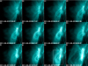 |
Fig. 8. Example of the evolution, at 131 Å, of a preexisting HFR whose formation was associated with a confined flare (PREC; event 25 in Table 1). The dotted curves delineate the outer edge of the HFR. The box in panel k marks the area used for the calculations presented in Fig. 9. The field of view is 300 × 300 arcsec2. See also the associated online movie. |
Event 25 was also presented in Paper I, where we had missed the early development of the HFR (we noted that “The first evidence of the hot flux rope appears around 10:24.”) because we used a 55-min-long sequence of 131 Å images that covered the interval from 10:09 to 11:04. This demonstrates that the use of rather limited time intervals in the study of flux rope formation times may lead to inaccurate conclusions.
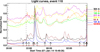
A PREC event that appeared even earlier (356 min), with respect to the eruptive flare, than event 25 is presented in Fig. 10 (event 118 of Table 1; see also the associated movie). Panel a shows the pre-event configuration. The first detection of the flux rope was made after 21:43 in conjunction with the development of a confined flare (see panel c). Although the GOES light curve does not show the flare onset (probably because of the elevated background level), it appears clearly in all AIA channels that we studied (see the light curves of Fig. 11). The early development of the flux rope (panels c–f), which consists of a blob on top of the flaring loops (i.e., its morphology was consistent with a flux rope seen edge-on; see Sect. 2), follows the development of the confined flare, which shows a prominent peak 40 min after its onset. During the decay phase of the flare, the flux rope cools down and becomes fainter until it cannot be traced in AIA images (panels g–j). In the extended interval between the end of the confined flare and the onset of the eruptive flare, the flux rope reappears for short periods, centered around 23:41, 01:31, 01:53, and 03:39 (see the associated movie), which coincide with local peaks in the light curves of the 131 Å and 94 Å emission (see Fig. 11). We conjecture that flaring activity provided plasma heating through magnetic reconnection. Unfortunately, due to the location of the HFR close to the limb, we cannot check whether reconnection also changes the magnetic flux of the flux rope, as has been found by Guo et al. (2013). The flux rope appears again just before the eruptive flare, in the course of which it rises (see panels k and l) until it leaves the field of view of the instrument.
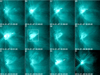 |
Fig. 10. Same as Fig. 8 but for event 118 in Table 1. The arrows mark the HFR. The field of view is 180 × 180 arcsec2. See also the associated online movie. |
In the description of events 25 and 118, we mentioned the existence of time intervals in which the flux ropes “disappeared” from the 131 Å images. The same was also true for their 94 Å emissions. Such time intervals were found in all PREC events at both 131 and 94 Å. These intervals start from about 20 min to more than 1.5 hours after the appearance of the PREC flux ropes and can last from about 30 min to more than 3.5 hours. Cooling of the flux ropes is a possible explanation for such behavior. The varying onset times of these intervals with respect to the appearance of the flux ropes may reflect different occurrence times of reconnection events, which could power the confined flare and heat the plasma.
Cargill (1994) assumed that loops impulsively heated to flare temperatures cool initially by conduction and at later times by radiation. The time scale of cooling due to thermal conduction is
 (1)
(1)
where k is the Boltzmann constant and n, T, and L are the number density, temperature, and characteristic length scale of the structure, respectively (e.g., Pagano et al. 2007). On the other hand, the time scale of radiative losses is
 (2)
(2)
where P(T) is the radiative loss function. Results for flux rope plasmas with different values of n and T, under the assumption of L ≈ 30 Mm (e.g., see Cheng et al. 2012; Patsourakos et al. 2013), are presented in Table 2. The value of n = 12 × 109 cm−3 has been taken from Syntelis et al. (2016), who performed differential emission measure analysis of two HFR events observed by the Hinode EUV Imaging Spectrometer (EIS) and AIA, while the value of n = 1.1 × 109 cm−3 is the average number density of HFRs derived by Cheng et al. (2012) using AIA data. A temperature of 8 MK is appropriate for HFRs visible in the 131 and 94 Å passbands for which the radiative loss function can be approximated by P(T) = 5.49 × 10⁻¹⁶T−1 (Klimchuk et al. 2008). The value of τc = 16 min deduced from the large number density appears broadly consistent with our observations, while both values of τr (i.e., 33 and 348 min) should be considered as upper limits because they do not take into account the conductive cooling of the plasma, which presumably occurred earlier. To this end, we also provide the values of τr for a lower temperature of 2.5 MK in Table 2. For that temperature, the approximate expression for P(T) becomes P(T) = 3.53 × 10⁻¹³T−3/2 (Klimchuk et al. 2008), and we obtain values of τr that are a factor of about 4 lower than before.
Cooling time scales of hot flux rope plasmas.
The cooling at the site of the confined flare is evident in the light curves of some PREC events (see Fig. 11 for an example), where the flare peak generally tends to appear progressively in passbands that probe cooler material (see Viall & Klimchuk 2012, 2013). In five of these events, the flux rope also appears, for limited time intervals, after the confined flare in some of the cooler passbands centered at 211 and 335 Å. Those were the PREC events whose formations were associated with the strongest confined flares, as judged by the maximum value of their intensity at 131 Å (see the relevant entries in the fifth column of Table 1). As a heating event becomes stronger, more plasma is evaporated and therefore one could anticipate higher densities of the cooling plasma. On the other hand, there was not a single case in which we could track the flux rope in cooler passbands throughout the interval of its disappearance from the 131 and 94 Å images. This could be attributed to the low density of the flux rope material (see Syntelis et al. 2016). The difficulty in observing cooling flux rope plasmas at temperatures of a few million K may also be related to the fact that during periods without flare activity, the active region differential emission measure peaks in that temperature range, thus making it possibly more difficult to detect the cooling of the flux rope plasma against a higher background.
5. Discussion and conclusions
This paper presents the first statistical survey of EUV observations to determine the formation times of eruptive HFRs relative to the CME initiation. We considered 34 M-class and X-class flares that occurred relatively close to the limb and involved hot channel or hot blob configurations, which were interpreted as HFRs in Paper I. Using uninterrupted sequences of 131 Å images that spanned more than eight hours, we determined the formation time of the HFRs using the same morphological criteria that we had used in Paper I. Our results are summarized in Table 3 and in the histogram of Fig. 12. Our main conclusions are as follows.
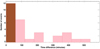 |
Fig. 12. Histogram of the number of events versus the time difference between the onset of the eruptive flare and the appearance of the HFR. |
Statistics of the patterns of HFR formation.
(1) Two thirds (20/30) of the events for which the formation time of the HFRs was unambiguously determined involved a preexisting HFR (that is, an HFR that was formed before the onset of the eruptive flare) whose formation was associated with the occurrence of a distinct confined flare (PREC events). There were four events with a preexisting HFR that was not formed in conjunction with a confined flare (PRE events) and six events in which the HFR was formed once the eruption was underway In the latter group, there was no evidence of prominence material in the 131 Å images (FLY events) in three of the events, while in the other three events there was (FLYP events).
(2) In the FLY and FLYP events, the time difference, Δt, between the onset of the eruptive flare and the appearance of the HFR is either zero or negative. After setting these negative values to zero, we found that the mean and median values of Δt for the whole population of events were 151 and 98 min, respectively.
(3) The time difference, Δt, was larger, in an average sense, in events that involved a PREC flux rope than in those that involved a PRE flux rope; in the former group, Δt ranged from 51 to 536 min, while in the latter it ranged from 3 to 39 min. Our sample is too small to know if we have two populations in a statistical sense. However, there is evidence that the formation patterns of HFRs either during or before eruptions do not show substantial differences when the appearance of the flux rope is not associated with any distinct confined flare activity. This conclusion is further reinforced if we take into account the uncertainties of 3–4 min and at least one minute (the latter being a lower limit) that are associated with the determination of the onset of the eruptions and the formation times of the HFRs, respectively (see Sect. 3). The segregation of the PREC events is also reflected in the histogram of Fig. 12; all but two of the 12 events that populate the leftmost bar of the histogram (brown color) are either FLY, FLYP, or PRE events, while the events that populate all the other bars (pink color) are exclusively PREC events.
(4) The existence of a significant population of preexisting HFRs that were formed well before the initiation of the eruptions (≳1 hour) is consistent with previous case studies on the formation times of sigmoidal EUV hot channel structures that were located close to disk center. These studies include Cheng et al. (2015), Chintzoglou et al. (2015), Joshi et al. (2015), Zhou et al. (2017), James et al. (2018), and Wang et al. (2019), who reported hot channel formation times relative to the onset of the eruptions of about 3–4.5, 11, 1.5, 2.5, 2, and 5 hours, respectively.
(5) We emphasize that the use of uninterrupted, long (more than 8 hours) sequences of images was essential for revealing the statistical prevalence of “truly” preexisting HFRs that were formed well before the onset of the eruptions. For example, if we had used one-hour-long sequences of images, as in Paper I, we would have missed the formation time of 18 HFRs because they appeared more than one hour before the onset of the corresponding eruptions. We also speculate that revisiting published case studies of HFRs that employed rather short sequences of images may also shift the formation of some flux ropes to earlier times with respect to the initiation of the eruptions (see also Sect. 4.3).
(6) It is possible that the percentage of truly preexisting HFRs that we reported are lower limits of the actual ones for the following reasons. (i) In three out of the six events with HFRs formed on the fly, there is evidence of prominence material in 131 Å images, which may indicate the presence of preexisting flux ropes (FLYP events of Sects. 3 and 4). Therefore, the only difference between such events and the events with preexisting HFRs may be the amount of heating available prior to the eruption. (ii) In all four events grouped as “uncertain” in Sect. 3, the HFRs were formed well before the onset of the eruption, but we were unable to unambiguously determine the time of their appearance. (iii) Only three PREC events contained a flux rope configuration seen face-on. Although this percentage (3/20) is similar to the percentage of flux ropes seen face-on that was reported in Paper I (9/45), we cannot exclude the possibility that, due to their poor visibility compared to flux ropes seen edge-on (see Paper I), we missed the early formation of some HFRs that initially appeared face-on.
(7) Not all confined flares recorded in the light curves we constructed were associated with the formation of flux ropes. It is difficult to establish a pattern or common characteristics for those that do, but this is a topic that deserves further investigation.
(8) Our results provide, on average, indirect support for CME initiation models that involve preexisting magnetic flux ropes that subsequently erupt, although for a minority of cases models in which the flux rope is formed during the eruption might be more appropriate. Due to the lack of suitable magnetic field data, it is difficult, and beyond the scope of this paper, to address the question about which events are initiated by ideal mechanisms and then pinpoint the relevant instability, or to speculate about the possible contribution of the tether-cutting scenario versus the breakout model. For limb events such as the ones we studied, these questions could be addressed in the future by combining the AIA observations with simultaneous vector magnetograms of the source region from the recently launched Solar Orbiter mission in quadrature or from an L4 or L5 mission.
Movies
Movie of Fig. 2 Access Supplementary Material
Movie of Fig. 5 Access Supplementary Material
Movie of Fig. 8 Access Supplementary Material
Movie of Fig. 10 Access Supplementary Material
Acknowledgments
We thank the referee for his/her constructive comments. A.N., X.C., and JZ. thank the ISSI team on “Decoding the Pre-Eruptive Magnetic Configuration of Coronal Mass Ejections”, led by S. Patsourakos and A. Vourlidas, for stimulating our research. AV is supported by NSF grants 80NSSC18K0622 and NNX17AC47G. X.C. is supported by NSFC Grants 11722325, 11733003, 11790303, 11790300, Jiangsu NSF Grant BK20170011, and the Alexander von Humboldt foundation. J.Z. is supported by NASA grant NNH17ZDA001N-HSWO2R.
References
- Amari, T., Luciani, J.-F., Aly, J.-J., & Tagger, M. 1996, A&A, 306, 913 [NASA ADS] [Google Scholar]
- Amari, T., Luciani, J. F., & Aly, J. J. 2004, ApJ, 615, 165 [NASA ADS] [CrossRef] [Google Scholar]
- Amari, T., Luciani, J. F., & Aly, J. J. 2005, ApJ, 629, 37 [CrossRef] [Google Scholar]
- Amari, T., Canou, A., Aly, J.-J., et al. 2018, Nature, 554, 211 [NASA ADS] [CrossRef] [Google Scholar]
- Archontis, V., & Török, T. 2008, A&A, 492, 35 [Google Scholar]
- Archontis, V., & Hood, A. W. 2012, A&A, 537, A62 [NASA ADS] [CrossRef] [EDP Sciences] [Google Scholar]
- Antiochos, S. K., DeVore, C. R., & Klimchuk, J. A. 1999, ApJ, 510, 485 [Google Scholar]
- Aulanier, G. 2014, in Nature of Prominences and their Role in Space Weather, eds. B. Schmieder, J. M. Malherbe, & S. T. Wu, IAU Symp., 300, 184 [Google Scholar]
- Aulanier, G., DeLuca, E. E., Antiochos, S. K., et al. 2000, A&A, 540, 1126 [Google Scholar]
- Brueckner, G. E., Howard, R. A., Koomen, M. J., et al. 1995, Sol. Phys., 162, 357 [NASA ADS] [CrossRef] [Google Scholar]
- Canou, A., Amari, T., Bommier, V., et al. 2009, ApJ, 693, L27 [NASA ADS] [CrossRef] [Google Scholar]
- Cargill, P. J. 1994, ApJ, 422, 381 [Google Scholar]
- Chandra, R., Mandrini, C. H., Schmieder, B., et al. 2017, A&A, 598, A41 [CrossRef] [EDP Sciences] [Google Scholar]
- Chen, P. F. 2011, Liv. Rev. Sol. Phys., 8, 1 [Google Scholar]
- Chen, H., Zhang, J., Cheng, X., et al. 2014a, ApJ, 797, L15 [CrossRef] [Google Scholar]
- Chen, B., Bastian, T. S., & Gary, D. E. 2014b, ApJ, 794, 149 [NASA ADS] [CrossRef] [Google Scholar]
- Chen, H., Zhang, J., Li, L., & Ma, S. 2016, ApJ, 818, L27 [NASA ADS] [CrossRef] [Google Scholar]
- Chen, B., Yu, S., Reeves, K. K., & Gary, D. E. 2020, ApJ, 895, L50 [CrossRef] [Google Scholar]
- Cheng, X., Zhang, J., & Ding, M. D. 2011, ApJ, 732, L25 [NASA ADS] [CrossRef] [Google Scholar]
- Cheng, X., Zhang, J., Saar, S. H., & Ding, M. D. 2012, ApJ, 761, 62 [NASA ADS] [CrossRef] [Google Scholar]
- Cheng, X., Zhang, J., Ding, M. D., Liu, Y., & Poomvises, W. 2013, ApJ, 763, 43 [NASA ADS] [CrossRef] [Google Scholar]
- Cheng, X., Ding, M. D., Zhang, J., Srivastava, A. K., Guo, Y., Chen, P. F., & Sun, J. Q. 2014a, ApJ, 789, L35 [CrossRef] [Google Scholar]
- Cheng, X., Ding, M. D., Zhang, J., Sun, X. D., Guo, Y., Wang, Y. M., Kliem, B., & Deng, Y. Y. 2014b, ApJ, 789, 93 [NASA ADS] [CrossRef] [Google Scholar]
- Cheng, X., Ding, M. D., Zhang, J., Vourlidas, A., Liu, Y. D., Olmedo, O., Sun, J. Q., & Li, C. 2014c, ApJ, 780, 28 [NASA ADS] [CrossRef] [Google Scholar]
- Cheng, X., Ding, M. D., & Fang, C. 2015, ApJ, 804, 82 [NASA ADS] [CrossRef] [Google Scholar]
- Cheng, X., Guo, Y., & Ding, M. D. 2017, ScChE, 60, 1383 [Google Scholar]
- Cheng, X., Zhang, J., Kliem, B., et al. 2020, ApJ, 894, 85 [Google Scholar]
- Chintzoglou, G., Patsourakos, S., & Vourlidas, A. 2015, ApJ, 809, 34 [NASA ADS] [CrossRef] [Google Scholar]
- Duan, A., Jiang, C., He, W., et al. 2019, ApJ, 884, 73 [CrossRef] [Google Scholar]
- Fan, Y., & Gibson, S. E. 2007, ApJ, 668, 1232 [Google Scholar]
- Forbes, T. G. 2000, J. Geophys. Res., 105, 23153 [NASA ADS] [CrossRef] [Google Scholar]
- Forbes, T. G., & Isenberg, P. A. 1991, ApJ, 373, 294 [Google Scholar]
- Forbes, T. G., & Priest, E. R. 1995, ApJ, 446, 377 [NASA ADS] [CrossRef] [Google Scholar]
- Georgoulis, M. K., Nindos, A., & Zhang, H. 2019, Phil. Trans. R. Soc. A: Math. Phys. Eng. Sci., 377, 20180094 [NASA ADS] [CrossRef] [Google Scholar]
- Gibson, S. E., & Low, B. C. 1998, ApJ, 493, 460 [NASA ADS] [CrossRef] [Google Scholar]
- Green, L. M., & Kliem, B. 2009, ApJ, 700, L83 [NASA ADS] [CrossRef] [Google Scholar]
- Green, L. M., Kliem, B., & Wallace, A. J. 2011, A&A, 526, A2 [NASA ADS] [CrossRef] [EDP Sciences] [Google Scholar]
- Green, L. M., Török, T., Vršnak, B., Manchester, W., & Veronig, A. 2018, Space Sci. Rev., 214, 46 [Google Scholar]
- Guo, Y., Ding, M. D., Cheng, X., et al. 2013, ApJ, 779, 157 [NASA ADS] [CrossRef] [Google Scholar]
- Hannah, I. G., Christe, S., Krucker, S., et al. 2008, ApJ, 677, 704 [NASA ADS] [CrossRef] [Google Scholar]
- Isenberg, P. A., Forbes, T. G., & Démoulin, P. 1993, ApJ, 417, 368 [Google Scholar]
- Jacobs, C., Poedts, S., & van der Holst, B. 2006, A&A, 450, 793 [NASA ADS] [CrossRef] [EDP Sciences] [Google Scholar]
- James, A. W., Green, L. M., Palmerio, E., et al. 2017, Sol. Phys., 292, 71 [NASA ADS] [CrossRef] [Google Scholar]
- James, A. W., Valori, G., Green, L. M., et al. 2018, ApJ, 855, L16 [NASA ADS] [CrossRef] [Google Scholar]
- Jiang, C., Wu, S. T., Feng, X., & Hu, Q. 2014, ApJ, 786, L16 [NASA ADS] [CrossRef] [Google Scholar]
- Joshi, N. C., Magara, T., & Inoue, S. 2014, ApJ, 795, 4 [CrossRef] [Google Scholar]
- Joshi, N. C., Liu, C., Sun, X., et al. 2015, ApJ, 812, 50 [Google Scholar]
- Karpen, J. T., Antiochos, S. K., & DeVore, C. R. 2012, ApJ, 760, 81 [NASA ADS] [CrossRef] [Google Scholar]
- Kliem, B., & Török, T. 2006, Phys. Rev. Lett., 96, 255002 [Google Scholar]
- Klimchuk, J. A. 2001, in Space Weather, eds. P. Song, H. J. Singer, & G. L. Siscoe (AGU), Geophys. Monograph Ser., 125, 143 [Google Scholar]
- Klimchuk, J. A., Patsourakos, S., & Cargill, P. G. 2008, ApJ, 682, 1351 [Google Scholar]
- Kumar, P., Yurchyshyn, V., Cho, K.-S., & Wang, H. 2017, A&A, 603, A36 [NASA ADS] [CrossRef] [EDP Sciences] [Google Scholar]
- Lemen, J. R., Title, A. M., Akin, D. J., et al. 2012, Sol. Phys., 275, 17 [Google Scholar]
- Li, L. P., & Zhang, J. 2013, A&A, 552, L11 [NASA ADS] [CrossRef] [EDP Sciences] [Google Scholar]
- Liu, C., Deng, N., Liu, R., et al. 2012, ApJ, 745, L4 [NASA ADS] [CrossRef] [Google Scholar]
- Liu, L., Cheng, X., Wang, Y., et al. 2018, ApJ, 867, L5 [NASA ADS] [CrossRef] [Google Scholar]
- López Ariste, A., Aulanier, G., Schmieder, B., & Sainz Dalda, A. 2006, A&A, 456, 725 [NASA ADS] [CrossRef] [EDP Sciences] [Google Scholar]
- Lynch, B. J., & Edmondson, J. K. 2013, ApJ, 764, 87 [NASA ADS] [CrossRef] [Google Scholar]
- Lynch, B. J., Antiochos, S. K., DeVore, C. R., Luhmann, J. G., & Zurbuchen, T. H. 2008, ApJ, 683, 1192 [NASA ADS] [CrossRef] [Google Scholar]
- MacNeice, P., Antiochos, S. K., Phillips, A., et al. 2004, ApJ, 614, 1028 [NASA ADS] [CrossRef] [Google Scholar]
- Mikić, Z., & Linker, J. A. 1994, ApJ, 430, 898 [Google Scholar]
- Moore, R. L., Sterling, A. C., Hudson, H. S., & Lemen, J. R. 2001, ApJ, 552, 833 [Google Scholar]
- Narukage, N., Sakao, T., Kano, R., et al. 2011, Sol. Phys., 269, 169 [NASA ADS] [CrossRef] [Google Scholar]
- Nindos, A., Patsourakos, S., Vourlidas, A., & Tagikas, C. 2015, ApJ, 808, 117 (Paper I) [NASA ADS] [CrossRef] [Google Scholar]
- O’Dwyer, B., Del Zanna, G., Mason, H. E., et al. 2010, A&A, 521, A21 [NASA ADS] [CrossRef] [EDP Sciences] [Google Scholar]
- Pagano, P., Reale, F., Orlando, S., & Peres, G. 2007, A&A, 464, 753 [NASA ADS] [CrossRef] [EDP Sciences] [Google Scholar]
- Patsourakos, S., Vourlidas, A., & Stenborg, G. 2013, ApJ, 764, 125 [NASA ADS] [CrossRef] [Google Scholar]
- Pesnell, W. D., Thompson, B. J., & Chamberlin, P. C. 2012, Sol. Phys., 275, 3 [Google Scholar]
- Reeves, K. K., & Golub, L. 2011, ApJ, 727, L52 [NASA ADS] [CrossRef] [Google Scholar]
- Roussev, I. I., Forbes, T. G., Gombosi, T. I., et al. 2003, ApJ, 588, 45 [Google Scholar]
- Roussev, I. I., Sokolov, I. V., Forbes, T. G., et al. 2004, ApJ, 605, 73 [Google Scholar]
- Schmieder, B., Aulanier, G., & Vršnak, B. 2015, Sol. Phys., 290, 3457 [Google Scholar]
- Shimizu, T. 1995, PASJ, 47, 251 [NASA ADS] [Google Scholar]
- Song, H. Q., Zhang, J., Chen, Y., & Cheng, X. 2014, ApJ, 792, L40 [NASA ADS] [CrossRef] [Google Scholar]
- Sterling, A. C., & Moore, R. L. 2004, ApJ, 602, 1024 [Google Scholar]
- Syntelis, P., Gontikakis, C., Patsourakos, S., & Tsinganos, K. 2016, A&A, 588, A16 [NASA ADS] [CrossRef] [EDP Sciences] [Google Scholar]
- Török, T., & Kliem, B. 2005, ApJ, 630, L97 [Google Scholar]
- Tripathi, D., Reeves, K. K., Gibson, S. E., Srivastava, A., & Joshi, N. C. 2013, ApJ, 778, 142 [NASA ADS] [CrossRef] [Google Scholar]
- Ugarte-Urra, I., Warren, H. P., & Winebarger, A. R. 2007, ApJ, 662, 1293 [Google Scholar]
- Vemareddy, P., & Zhang, J. 2014, ApJ, 797, 80 [CrossRef] [Google Scholar]
- Veronig, A. M., Podladchikova, T., Dissauer, K., et al. 2018, ApJ, 868, 107 [Google Scholar]
- Viall, N. M., & Klimchuk, J. A. 2012, ApJ, 753, 35 [NASA ADS] [CrossRef] [Google Scholar]
- Viall, N. M., & Klimchuk, J. A. 2013, ApJ, 771, 115 [NASA ADS] [CrossRef] [Google Scholar]
- Wang, W., Zhu, C., Qiu, C., et al. 2019, ApJ, 871, 25 [NASA ADS] [CrossRef] [Google Scholar]
- Xue, Z., Yan, X., Cheng, X., et al. 2016, Nat. Commun., 7, 11837 [Google Scholar]
- Xue, Z., Yan, X., Yang, L., et al. 2017, ApJ, 840, L23 [NASA ADS] [CrossRef] [Google Scholar]
- Yan, Y., Deng, Y., Karlický, M., Fu, Q., Wang, S., & Liu, Y. 2001, ApJ, 551, L115 [NASA ADS] [CrossRef] [Google Scholar]
- Yardley, S. L., Green, L. M., Williams, D. R., et al. 2016, ApJ, 827, 151 [NASA ADS] [CrossRef] [Google Scholar]
- Yashiro, S., Gopalswamy, N., Michalek, G., et al. 2004, J. Geophys. Res. (Sp. Phys.), 109, A07105 [Google Scholar]
- Zhang, J., Cheng, X., & Ding, M.-D. 2012, Nat. Commun., 3, 747 [NASA ADS] [CrossRef] [Google Scholar]
- Zhou, Z. J., Zhang, J., Wang, Y. M., et al. 2017, ApJ, 851, 133 [CrossRef] [Google Scholar]
All Tables
All Figures
|
Fig. 1. Events, at 131 Å, with HFRs formed during the eruption with (middle and right-hand columns; FLYP) and without (left column; FLY) preexisting prominence material. Top row: snapshots of the pre-event configuration. Bottom row: snapshots after the appearance of the HFRs. The images of the left-hand, middle, and right-hand columns correspond to events 70, 5, and 99 in Table 1, respectively. The arrows mark the HFRs. The field of view in each image is 300 × 300 arcsec2. |
| In the text | |
|
Fig. 2. Example of the formation, at 131 Å, of an HFR during the eruption (FLY; event 89 in Table 1). The arrows mark the HFR. The box in panel j marks the area used for the calculations presented in Fig. 3. The field of view is 300 × 300 arcsec2. See also the associated online movie. |
| In the text | |
|
Fig. 3. Light curves in 94, 131, 171, 193, 211, 304, and 335 Å AIA passbands from the region marked with the box shown in Fig. 2j as well as in the GOES 1–8 Å channel. All curves are normalized to their maximum values. The vertical dashed line marks the first appearance of the HFR. The arrows just above the horizontal axis mark the times of the images displayed in Fig. 2. |
| In the text | |
|
Fig. 4. Events, at 131 Å, with preexisting HFRs whose formations were not associated with confined flares (PRE). Top row: snapshots of HFRs observed a few minutes after their appearance. Bottom row: the flux ropes of the top row observed at a later stage. The images of the left- and right-hand columns correspond to events 35 and 107 in Table 1, respectively. The arrows mark the HFRs. The field of view in each image is 300 × 300 arcsec2. |
| In the text | |
|
Fig. 5. Example of the evolution, at 131 Å, of a preexisting HFR whose formation was not associated with a confined flare (PRE; event 61 in Table 1). The arrows mark the HFR. The box in panel j marks the area used for the calculations presented in Fig. 6. The field of view is 300 × 300 arcsec2. See also the associated online movie. |
| In the text | |
|
Fig. 7. Same as Fig. 4 but for preexisting HFRs whose formations were associated with confined flares (PREC). The images in the left-hand, middle, and right-hand columns correspond to events 81, 97, and 133 in Table 1, respectively. The field of view in each image is 300 × 300 arcsec2 except in those of the middle column where it is 360 × 360 arcsec2. |
| In the text | |
|
Fig. 8. Example of the evolution, at 131 Å, of a preexisting HFR whose formation was associated with a confined flare (PREC; event 25 in Table 1). The dotted curves delineate the outer edge of the HFR. The box in panel k marks the area used for the calculations presented in Fig. 9. The field of view is 300 × 300 arcsec2. See also the associated online movie. |
| In the text | |
|
Fig. 10. Same as Fig. 8 but for event 118 in Table 1. The arrows mark the HFR. The field of view is 180 × 180 arcsec2. See also the associated online movie. |
| In the text | |
|
Fig. 12. Histogram of the number of events versus the time difference between the onset of the eruptive flare and the appearance of the HFR. |
| In the text | |
Current usage metrics show cumulative count of Article Views (full-text article views including HTML views, PDF and ePub downloads, according to the available data) and Abstracts Views on Vision4Press platform.
Data correspond to usage on the plateform after 2015. The current usage metrics is available 48-96 hours after online publication and is updated daily on week days.
Initial download of the metrics may take a while.