| Issue |
A&A
Volume 642, October 2020
|
|
|---|---|---|
| Article Number | A97 | |
| Number of page(s) | 12 | |
| Section | Stellar structure and evolution | |
| DOI | https://doi.org/10.1051/0004-6361/202038702 | |
| Published online | 09 October 2020 | |
Formation of sdB-stars via common envelope ejection by substellar companions
1
Heidelberger Institut für Theoretische Studien, Schloss-Wolfsbrunnenweg 35, 69118 Heidelberg, Germany
e-mail: This email address is being protected from spambots. You need JavaScript enabled to view it.
2
Astronomisches Rechen-Institut, Zentrum für Astronomie der Universität Heidelberg, Mönchhofstr. 12-14, 69120 Heidelberg, Germany
3
Max Planck Computing and Data Facility, Gießenbachstr. 2, 85748 Garching, Germany
4
Institut für Physik und Astronomie, Universität Potsdam, Haus 28, Karl-Liebknecht-Str. 24/25, 14476 Potsdam-Golm, Germany
5
Max-Planck-Institut für Astrophysik, Karl-Schwarzschild-Str. 1, 85748 Garching, Germany
6
Institut für Theoretische Astrophysik, Zentrum für Astronomie der Universität Heidelberg, Philosophenweg 12, 69120 Heidelberg, Germany
Received:
19
June
2020
Accepted:
10
August
2020
Abstract
Common envelope (CE) phases in binary systems where the primary star reaches the tip of the red giant branch are discussed as a formation scenario for hot subluminous B-type (sdB) stars. For some of these objects, observations point to very low-mass companions. In hydrodynamical CE simulations with the moving-mesh code AREPO, we test whether low-mass objects can successfully unbind the envelope. The success of envelope removal in our simulations critically depends on whether or not the ionization energy released by recombination processes in the expanding material is taken into account. If this energy is thermalized locally, envelope ejection eventually leading to the formation of an sdB star is possible with companion masses down to the brown dwarf range. For even lower companion masses approaching the regime of giant planets, however, envelope removal becomes increasingly difficult or impossible to achieve. Our results are consistent with current observational constraints on companion masses of sdB stars. Based on a semi-analytic model, we suggest a new criterion for the lowest companion mass that is capable of triggering a dynamical response of the primary star thus potentially facilitating the ejection of a CE. This gives an estimate consistent with the findings of our hydrodynamical simulations.
Key words: hydrodynamics / binaries : close / subdwarfs / brown dwarfs
© ESO 2020
1. Introduction
Hot subluminous B-type (sdB) stars are helium-core-burning stars that contain almost no hydrogen. They reach hot surface temperatures of about 2 × 10⁴ K to 4 × 10⁴ K, which places them on the blue end of the horizontal branch (Heber 1986). To form sdB stars, almost all of the hydrogen envelope of the progenitor must be removed by the time the helium ignition is triggered in the core. When this process commences, it thus has most likely evolved to the tip of the red giant branch (RGB).
A natural mechanism for removing the hydrogen envelope is the interaction with a binary companion. About 50% of sun-like stars evolve alongside a companion and this fraction is even higher for more massive stars (Duchêne & Kraus 2013; Moe & Di Stefano 2017). When one star in a close binary system reaches the RGB, it expands rapidly, thus overfilling its Roche lobe (RL), and can trigger unstable mass transfer. If the receiving companion cannot accrete all of this material, it will be engulfed and a common envelope (CE) is formed (Paczyński 1976) around the two compact stellar cores. These cores spiral inward and transfer angular momentum and energy to the envelope material. As a result, the envelope expands and might be partially or even completely ejected from the system (Ivanova et al. 2013). The separation between the cores is greatly reduced and a close binary forms.
Observations have indeed shown that 40% to 70% of single-lined sdB stars exist in close binary systems with periods ranging from 0.03 d to 10 d (Maxted et al. 2001). This strongly suggests a previous CE phase, in which the orbital separation is reduced and the red giant (RG) progenitor loses most of his hydrogen-rich envelope material in the interaction with its companion (Han et al. 2002, 2003). Surprisingly, several sdB binaries with companions in the brown dwarf (BD) regime have been found in recent surveys (Geier et al. 2011; Schaffenroth et al. 2014, 2015). This raises the question of whether a CE interaction with such low-mass companions can indeed trigger successful envelope ejection. Based on estimates assuming a one-dimensional (1D) static structure of the primary, Soker (1998) and Nelemans & Tauris (1998) argue that companions with masses lower than about 10−2 M⊙ evaporate or lose their mass in RL overflow before completely ejecting the envelope material.
Such estimates bear large uncertainties because they do not follow the hydrodynamic evolution and call for a closer investigation. The dynamics of common envelope evolution (CEE) can only be captured self-consistently in three-dimensional (3D) hydrodynamical simulations. With the wide range of spatial scales involved and the need to follow the system over many orbits, such simulations pose substantial challenges to numerical approaches. Smoothed-particle hydrodynamics (SPH) offers a way to account for the “Lagrangian nature” of the problem, but it usually lacks spatial resolution in the dilute stellar envelopes. Moving mesh techniques, that combine the efficiency of (nearly) Lagrangian methods with the accuracy of grid-based hydrodynamics solvers, are an improvement (Ohlmann et al. 2016a,b; Prust & Chang 2019; Sand et al. 2020). Despite recent progress in numerical techniques and available computational resources, a fundamental question of CEE remains unanswered: How is the envelope ejected? If driven by the release of orbital energy only, the ejection remains incomplete in all published CE simulations (for instance Ricker & Taam 2012; Passy et al. 2012; Ohlmann et al. 2016a; Reichardt et al. 2020; Sand et al. 2020). Additional physics seems to be required for a successful envelope removal. The ionization energy stored in the envelope will be released by recombination processes provided that the material expands sufficiently. If thermalized locally, this energy leads to further unbinding of material (Nandez et al. 2015; Nandez & Ivanova 2016; Prust & Chang 2019; Reichardt et al. 2020) and a complete envelope ejection seems possible.
No hydrodynamic CE simulations have previously been carried out in the context of the formation of sdB stars. We present such simulations aiming to determine if substellar companions are sufficient to trigger a significant unbinding of the envelope material in cases where the primary star is at the tip of its RGB. In the subsequent sections, we explain the methods and the setup of our simulations (Sect. 2) and present their results (Sect. 3). Based on these results, we develop a semi-analytic model for the inspiral of the stellar cores (Sect. 3.5), discuss the fate of the companion, and compare our results to observations (Sect. 4) before concluding (Sect. 5).
2. Methods
Following the work of Ohlmann et al. (2016a, b, 2017), we employed the moving-mesh magnetohydrodynamics code AREPO (Springel 2010; Pakmor et al. 2011; Pakmor & Springel 2013) to simulate the CE phase in a system composed of a primary star at the tip of its RGB and a compact low-mass companion. This code is particularly well-suited for this task because of its shock capturing abilities and the excellent conservation of angular momentum and energy. It allows for arbitrary refinement criteria to achieve higher resolution in specific areas. For most of our simulations, we used the OPAL equation of state (EoS; Rogers et al. 1996; Rogers & Nayfonov 2002). It accounts for ionization effects and allows us to track the release of recombination energy. This energy is, in our current implementation, assumed to be thermalized locally. For comparison, one simulation was carried out with an ideal gas EoS as detailed by Ohlmann et al. (2016a, b).
2.1. Red giant star model
With the stellar evolution code MESA (Paxton et al. 2013, 2015) in version 6208, we created a suitable RG progenitor model as the primary star (denoted with subscript 1 in the following) for the subsequent binary simulations. A 1 M⊙ zero-age main sequence star was evolved until the tip of the RGB. The metallicity was set to Z = 0.02, a mixing length parameter of αMLT = 2 was applied, and the Reimers prescription with η = 0.5 was used for RG winds. Due to mass loss via winds, we reach a stellar model that has a total mass of M1 = MRG = 0.77 M⊙, a radius of R1 = RRG = 173 R⊙, a core mass of Mcore = 0.47 M⊙, and an envelope mass of Menv = 0.30 M⊙.
The 1D MESA profile was then mapped onto a 3D grid following the procedure described in Ohlmann et al. (2017). We cut out the core at five percent of the radius of the MESA model and replaced it with a point mass that only interacts gravitationally, henceforth called “core particle”. When combining a grid-based representation of matter with point particles, the gravitational potential has to be softened (Springel 2010). This is the case in our simulations and we set the initial softening length to h = 3.1 R⊙.
To obtain a stellar model in hydrostatic equilibrium (HSE) where
 (1)
(1)
a modified Lane-Emden equation was solved to create a profile with a smooth transition between the core and the envelope (Ohlmann et al. 2017).
2.2. Relaxation
The spatial resolution is coarser in our 3D setup than in the 1D stellar evolution model, resulting in discretization errors. As a consequence, spurious motions arise in the mapped stellar structure. To restore HSE, we carried out a relaxation run of the mapped stellar model for ten dynamical timescales tdyn, which corresponds to 930 d. Velocities were damped by a constant factor during the first 2 tdyn and then constantly reduced until we reached t = 5 tdyn. For the remaining 5 tdyn, the damping was completely shut off which allowed us to check if the star stays stable in the relaxed configuration.
In the top panel of Fig. 1, the Mach number, the ratio between the absolute value of the local fluid velocity v and the speed of sound cs, Ma ≡ v/cs, in the mapped stellar model is plotted over the radius at different times. The inner part of the star stays subsonic with Ma ∼ 0.1. This shows that spurious velocities were damped successfully and the star’s envelope settles into a stable state. For technical reasons, the grid outside the star cannot be empty but has to be filled with low-density material. We chose a uniform background density of ρbg = 10−16 g cm−3, and the material is not in HSE. Consequently, in these regions, Mach numbers above 0.5 occur, but because these flows contain only 6.3 × 10⁻⁴ M⊙, they are irrelevant for the dynamics of the stellar envelope.
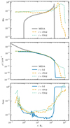 |
Fig. 1. Mach number Ma, density ρ, and relative deviation from HSE ΔHSE according to Eq. (2) over radius of the relaxed giant at the tip of the RGB. The quantities are binned over the radius and averaged in shells. |
The middle panel of Fig. 1 shows that the density profile does not change over time after we stopped the damping. We observe some expansion of surface material. This is caused by the steep initial pressure gradient, that cannot be fully resolved, which makes it impossible to fulfill the condition of HSE (1) for the original profile. Therefore, the relaxed profile settles into a new equilibrium with shallower surface gradients. Still, no mass is lost from the system and the original profile of the MESA output is well represented in the inner parts of the star, where most of the mass is concentrated.
In the bottom panel of Fig. 1, the relative difference between both sides of the HSE Eq. (1),
 (2)
(2)
is shown. Throughout most of the envelope, deviations from HSE stay at low values of ΔHSE ≈ 0.02. Near the center, close to the core particle, the error increases due to the slight decrease in density, as well as close to the surface due to the expansion. We computed a sphere centered on the core particle that contains 99.9% of the mass of the initial RG to define a final radius of R1 = RRG = 118 R⊙ at the end of the relaxation.
This shows that the relaxed model represents a star at the tip of the RGB. It stays stable over sufficiently many dynamical timescales to simulate the subsequent CE phase in a binary system.
2.3. Binary simulations
To setup our binary simulations, we placed a compact companion – denoted with subscript 2 in the following and technically realized as a second core particle of mass M2 – at an orbital separation a that corresponds to 80% of the RL radius. The binary components were placed on a Kepler orbit at a frequency of
 (3)
(3)
where G is the gravitational constant. To facilitate the inspiral, we imposed a corotation factor of χ = 0.95, so that initial velocity of the envelope is given by:
![Mathematical equation: $$ \begin{aligned} \boldsymbol{\nu }_\mathrm{env} = \chi \left( \boldsymbol{\Omega } \times [\boldsymbol{r} - \boldsymbol{r}_\mathrm{core} ] \right). \end{aligned} $$](/articles/aa/full_html/2020/10/aa38702-20/aa38702-20-eq4.gif) (4)
(4)
Here, rcore is the position of the RG core and Ω points into the z-direction.
We note that an earlier start of the simulations, close to the onset of Roche-lobe overflow, would be desirable, but it is prevented by the slow initial evolution of the considered system. Until plunge-in of the companion into the primary star, many orbits would have to be covered. The excellent angular momentum conservation of the moving-mesh code AREPO allows us to follow this evolution in principle, but the computational expense is prohibitive. The error in orbital energy introduced by placing the companion at 80% RL radius is on the order of one percent and therefore acceptable. Moreover, even in the chosen initial setup, it takes several orbits before the separation of the cores shrinks significantly. This leaves enough time for the stellar envelope to adjust to the modified effective potential after adding the companion.
In our simulations, we solved for full magnetohydrodynamics. Following Ohlmann et al. (2016b), the magnetic field of the RG star was initialized as dipole along the z-axis with 10−6 G at the pole. In our current treatise, however, we focus on the hydrodynamical evolution. The magnetic fields in our simulations are dynamically irrelevant and will be discussed in a forthcoming publication.
3. Results
In this section, we present the results of our 3D hydrodynamical CE simulations. All are based on the same initial MESA model for the RG primary star. Some general features of the dynamics are described in Sect. 3.1 based on a “reference simulation” with a companion mass of M2 = 0.08 M⊙. We then vary model parameters of the reference run independently: the spatial resolution around the core particles (Sect. 3.2) to test numerical convergence of the simulation and the EoS (Sect. 3.3) to investigate the effect of recombination energy release on envelope ejection. Based on the results of these runs, we carry out simulations, which explore the effect of the most important physical parameter of the systems under consideration – the mass of the companion – in a setup otherwise identical to the reference run (Sect. 3.4). Finally, we present a semi-analytic model that yields a new criterion for determining the lowest companion mass that is still capable of triggering envelope ejection (Sect. 3.5).
3.1. Reference simulation
For the reference run we choose a companion mass of M2 = 0.08 M⊙, implying a mass ratio of the companion to the primary star of q ≡ M2/M1 = 0.01. The companion is placed at a distance of ai = 164 R⊙ to the center of the RG (the initial period at the start of our simulation is Pi = 329d) and the OPAL EoS is applied. The companion spirals in, thereby ejecting a large fraction of the envelope. We follow this process in our simulation until t = 955d. At this point, we terminate the simulation because the time steps become prohibitively small to follow the further evolution. The reason for the decreasing time step is that we reduce the softening length around the core particles when they approach each other to avoid overlap. The number of grid cells per softening length is kept constant and, due to the CFL criterion (Courant et al. 1928), the time step must be reduced. During the complete run, the relative error amounts to 0.6% in the total energy and to 1.3% in angular momentum.
In Fig. 2, density slices through the orbital plane at different times are shown. During the first orbit, the structure of the RG remains almost unperturbed. Between t = 0 d and t ∼ 189 d, the companion accumulates mass in its wake and forms a tidal arm in the envelope material. The inspiral enters a faster phase and shear instabilities emerge at the edge of the tidal arm. From t ∼ 600 d to t ∼ 750 d, a layered structure emerges with shear instabilities between the adjacent layers. At the end of the simulation at t = 955 d, the initial structure of the RG is completely disrupted and a large fraction of the initial envelope has been removed.
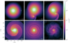 |
Fig. 2. Time series of density snapshots in the orbital plane at different times. The positions of the cores of the RG primary and the 0.08 M⊙ companion are marked by an × and + respectively. Each frame is centered on the center of mass of the binary system. |
In Fig. 3, we show the evolution of the orbital separation a. At t = 161 d, the rate of orbital decay ȧ/a surpasses 0.1 and thus initializes the phase of rapid inspiral, that stops at t = 695 d at an orbital separation of a ≈ 20 R⊙. The separation decreases at a slower rate until it reaches a = 10.4 R⊙ at the end of the simulation.
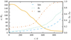 |
Fig. 3. Orbital separation a between companion and core of the RG over time t for a companion mass of 0.08 M⊙ (solid, left axis) and ejected mass fractions f according to the three criteria based on the kinetic (“kin”), thermal (“th”), and internal (“int”) energy as defined in the text (dashed, right axis). |
The fraction of unbound mass is plotted as a function of time in Fig. 3. We apply three different criteria to determine if mass is unbound, all based on the energy budget of the envelope material: The “kinetic energy criterion” counts mass as unbound if ekin+epot > 0, the “thermal energy criterion” if ekin+epot+eth > 0, and the “internal energy criterion” if ekin+epot+eint > 0, where ekin, epot, eth, and eint denote the kinetic, the potential gravitational, the thermal, and the internal energy of the gas, respectively. The internal energy includes both the thermal and the ionization energy of the gas. These criteria provide different estimates of the unbound mass. We refer to the ratio of unbound mass to the initial envelope mass Menv under the respective criterion as fkin, fth, and fint.
The kinetic energy criterion regards material as unbound only if its kinetic energy has overcome the gravitational binding energy. The other energy components, however, may ultimately be converted into kinetic energy and thus contribute to mass ejection, although this has not happened yet at the instant of measurement. The unbound mass fractions are still rising at the end of our simulation for both the kinetic and the thermal energy criteria. The orbital shrinkage has flattened out and thus orbital energy release ceases its contribution to envelope ejection. This shows that the conversion of thermal and ionization energy is still ongoing. Therefore, the kinetic energy criterion certainly underestimates the amount of material that can be unbound and provides a conservative lower limit. The ionization energy criterion assumes that all energy released in recombination processes can be used for envelope ejection. It provides an optimistic upper limit for mass ejection, because some of the energy may be transported away by radiation and/or convection (Grichener et al. 2018; Sabach et al. 2017; Wilson & Nordhaus 2019, 2020). The unbound mass according to the thermal energy criterion is a compromise between these two limiting cases and we will use it as a fiducial value. The final verdict on unbound mass requires us to follow the evolution until envelope ejection stalls for the kinetic energy criterion when also including radiation and convection effects.
We attribute the initial small offset in Fig. 3 in the unbound mass for both the thermal and the internal energy criterion to a readjustment of the energy contributions when placing the core particle representing the companion onto the grid containing the relaxed progenitor star. During the inspiral, the unbound masses determined with the kinetic and the thermal energy criterion both increase at a low rate, that grows after the orbit is stabilized. This is expected, because the ionization energy of the gas is only converted into thermal and kinetic energy when the envelope has significantly expanded and cooled. Assuming that all of the ionization energy will be used eventually, we obtain a fraction of unbound mass of fint = 99.7%. The thermal energy criterion yields fth = 77.8% of unbound gas and is still increasing steeply at the end of the run, because ionization energy is still being converted into thermal energy. This strongly suggests that further mass unbinding will take place. Consequently, even low-mass companions appear to suffice to completely unbind the envelope of the RG and form sdB systems.
3.2. Resolution study
For the CE dynamics, the transfer of orbital energy and angular momentum from the cores to envelope gas is critical. This proceeds around the cores. It is therefore necessary to sufficiently resolve the regions around the core particles in our simulations. As a test, we conduct a number of simulations with varying spatial resolution. The initial total number of cells in our simulation domain is approximately 2.4 × 10⁶. These parameters are applied to all simulations presented in this work. Using a special refinement criterion of AREPO, we vary the number of cells per softening length nc around the core particles between 10 and 40 and compare the evolution of the system. Except for nc, we use setups identical to the reference simulation of Sect. 3.1. We summarize the convergence test runs in Table 1. Because the refinement criterion produces additional grid cells around the core particles, the final total number of cells Nf in the simulation domain is larger by 37% for the highest-resolved run compared to that with the lowest resolution (see Table 1). This implies a growth in computational cost and for this reason the run with nc = 40 terminates at t = 955 d, while the other three extend to t = 1000 d.
Overview of the results of the resolution runs.
In the lower panel of Fig. 4, the orbital separation between the core particles is plotted over time. The final separations af and periods Pf are given in Table 1. The results of the simulations with nc = 40 and nc = 30 and the two simulations with nc = 20 and nc = 10 are qualitatively and quantitatively different. Overall, the two highest-resolved simulations are similar in their orbital evolution. The values of the final unbound mass fractions according to the thermal energy criterion and also the final orbital parameters are very close. This indicates that they are numerically converged. Both 10 and 20 cells per softening length are insufficient to capture the orbital energy and angular momentum transfer between the companion and the surrounding cells, which results in incomplete inspirals. More mass is unbound earlier in the simulations with low resolution, probably due to under-resolved gravitational interaction of the core particles. This can lead to spurious velocities that inject kinetic energy. It is interesting to note that the lowest-resolved simulation shows the largest mass ejection. This emphasizes the danger of wrong conclusions drawn from under-resolved CE simulations and underlines the necessity of through convergence studies.
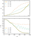 |
Fig. 4. Upper panel: fraction of unbound mass fth under the thermal energy criterion over time. The legend denotes the imposed number of cells nc per softening length. Lower panel: separation between the core particles is shown. |
All simulations conserve angular momentum and total energy relatively well, which is a necessary prerequisite for meaningful physical results, but, as demonstrated here, not a guarantee for numerical convergence. Table 1 summarizes the relative energy errors  , with E0 and Ef denoting the initial and final values of total energy in our simulation domain, and the analogously defined relative errors in total angular momentum
  .
.
From our test simulations, it is clear that the gravitational softening length has to be resolved with at least 30 cells. To be on the safe side, we opt for the highest resolution with nc = 40 in all simulations presented below. This ensures numerically converged results with favorable angular momentum and energy conservation.
3.3. The influence of ionization energy
To analyze the influence of recombination energy release on mass ejection, we repeat our reference run discussed in Sect. 3.1 with an ideal gas EoS thus ignoring ionization effects. We compare the results with our reference run, that employs the OPAL EoS and assumes local thermalization of recombination energy without cooling losses. Starting out from the same MESA model, the relaxation procedure outlined in Sect. 2.2 is repeated, but this time employing an ideal gas EoS. With the thus obtained RG star model, a binary system is set up adopting the same companion mass of M2 = 0.08 M⊙ and the same initial orbital parameters as in our reference simulation.
Figure 5 compares the evolution of unbound mass fraction according to the thermal energy criterion for both simulations. We reach a final value of fth = 77.8% in the reference run accounting for ionization effects, and the value is still increasing at the end of the simulation. In contrast, very little mass is ejected when applying the ideal gas EoS. Here, only fth = 7.3% are unbound at the end of the simulation and this fraction is hardly increasing any longer.
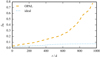 |
Fig. 5. Evolution of the fraction of the unbound mass fth assuming the thermal energy criterion for simulations with different EoS. |
This clearly emphasizes the importance of ionization energy and recombination processes for the ejection of the envelope for the considered case with M2 = 0.08 M⊙. Companions of even lower masses can certainly not eject the envelope when only tapping the orbital energy reservoir. As mentioned above, recombination energy is released when the gas of the envelope has sufficiently expanded and cooled to allow for electron captures. This is reflected in the fact that the unbinding only starts when the inspiral is already well underway. Since the envelope of the progenitor RG is only weakly bound, even small perturbations by low-mass companions cause a significant release of ionization energy that can ultimately lead to a nearly complete unbinding.
Figure 6 illustrates the final state of the two simulations. Its Panel b shows a density slice through the orbital plane at the end of the simulation with the OPAL EoS where ionization energy is included. Comparing with the initial RG primary in panel a shows that outer envelope is largely lost and the low density of the remaining material exhibits an irregular pattern. In contrast, the envelope material of the RG for the run without ionization effects in panel c is notably less disrupted and smoother. The envelope has expanded (cf. panel a), but since ionization energy is not taken into account, no recombination energy can be released and only a small amount of mass is unbound.
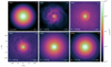 |
Fig. 6. Density snapshots in the orbital plane for different systems. Panel a: initial state of the primary RG star before a companion is added. Here, the time indicates that of the relaxation run. For the binary simulations in (panels b–f), the mass of the companion is given on the bottom left side of each panel, the time after adding the companion at the bottom right and the equation of state at the top left. The positions of the cores of the RG primary star and the companion are marked by an × and + respectively. Each frame is centered on the center of mass of the binary system. |
3.4. Varying companion masses
Overview of the simulation runs with different companion masses.
To study the influence of the companion’s mass on the envelope ejection, we conduct further simulations with identical setups as for the reference run in Sect. 3.1, but with lower M2 (see Table 2). With its 0.08 M⊙, companion of the reference simulation marks the limit above which hydrogen burning ignites and the objects become true stars. With our parameter study, we map out the mass range of BDs down to the most massive giant planets with M ≲ 0.01 M⊙. Table 2 summarizes parameters of our simulations. For comparison, we also include our simulation with the ideal gas EoS. In all runs, relative error in energy stays below 1% and in angular momentum under 2%. We list the initial separations between the core particles ai and the initial orbital periods Pi, as well as the corresponding values at the end of the respective simulations (af and Pf).
The top panel of Fig. 7 shows the evolution of the fraction of unbound mass fth according to the thermal energy criterion. Higher companion masses cause stronger perturbation of the envelope and lead to increased mass ejection. However, for masses as low as M2 = 0.05 M⊙ (q = 0.06), 52.1% of the envelope become unbound under the thermal energy criterion until the end of our simulation. It is also clear that material is still being ejected from the system at this point. If we apply the internal energy criterion which also accounts for ionization energy, the fraction increases to fint = 98.1% (see Table 2). The simulation with the lowest companion mass, however, shows a different picture (see upper panel of Fig. 7): the unbound mass according to the thermal energy criterion quickly reaches about 10% and then stagnates. Only 16.6% of the envelope mass is unbound at the end of the simulation. When employing the internal energy criterion, we find fint = 0.46, implying that even if all available ionization energy is used, less than half of the envelope will eventually become unbound.
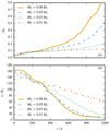 |
Fig. 7. Fraction of unbound mass fth according to the thermal energy criterion and orbital separation a between the core particles over time for simulations with the indicated companion masses M2. |
In the bottom panel of Fig. 7, the orbital separation between the core particles over time is plotted. While for the runs with the companion masses of 0.08 M⊙ and 0.05 M⊙ the separation between the core particles shows a qualitatively similar evolution, we see a distinct behavior for the companion with the lowest mass of 0.01 M⊙, where the orbital separation slowly but steadily decreases. These results indicate that around M2 = 0.03 M⊙ there is a companion mass threshold below which the dynamic interaction with the envelope is not strong enough to trigger significant envelope ejection (we discuss this further in Sect. 3.5).
This qualitatively different behavior can also be seen when comparing the density slices through the orbital plane at the end of the different simulations in Fig. 6. In panel a, the final state of the RG at the end of the relaxation run is given before placing the companion. As discussed above, a direct comparison of the relaxed model and the final state after the binary interaction with the M2 = 0.08 M⊙ (q = 0.10) companion makes the degree of perturbation of the envelope material apparent. Large scale instabilities have emerged and the smooth envelope is notably disrupted. The same can be observed for a companion mass of M2 = 0.05 M⊙ (q = 0.06), which is shown in panel d. However, the disruption in the inner part is not as strong and more material remains in the outer regions. This is not surprising considering the slower mass ejection in this case (see top panel of Fig. 7). As the unbound mass fraction fth is still increasing and fint ≈ 1, this marks only a snapshot in an evolution that ultimately will lead to almost complete envelope removal. This is different for the two lower companion masses. Their density slices in panels e and f of Fig. 6 display a less perturbed envelope. While layered spiral structures have emerged, no large scale perturbations occur. For the companion mass of M2 = 0.03 M⊙ (q = 0.04), the radius of the star appears to have slightly expanded, but for M2 = 0.01 M⊙ (q = 0.01) the expansion is marginal if present at all (see Sect. 3.5).
3.5. Minimum mass for envelope ejection
We have seen from our simulations that lower-mass companions eject less mass (Table 2 and Fig. 7). Even more so, the runs with companion masses of 0.03 M⊙ and 0.01 M⊙ have envelope ejection fractions of fth ≲ 20% over the course of our computations. This suggests that there exist a minimum companion mass below which the envelope of the RGB star is not perturbed strongly enough to cause significant envelope ejection. To further illuminate this lower mass threshold qualitatively, we consider a companion of mass M2 orbiting in the unperturbed envelope of our RGB star under the influence of a drag force (see also MacLeod & Ramirez-Ruiz 2015; MacLeod et al. 2017; Chamandy et al. 2019),
 (5)
(5)
In this equation, vrel is the relative velocity of the companion with respect to the bulk rotational velocity of the RGB star’s envelope, ρ and cs are the local density and sound speed in the unperturbed RGB star, respectively, and Ra a mass-accretion radius that we approximate by Bondi–Hoyle–Littleton theory (Bondi & Hoyle 1944; Bondi 1952),
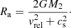 (6)
(6)
We further multiply the drag force by a drag coefficient Cd such that we finally have
 (7)
(7)
We initially place the companion as in the AREPO runs (that is, at the same initial orbital separation with an initial velocity according to a Keplerian orbit) and assume that the RGB star’s envelope rotates as a solid body that is in 95% co-rotation with the companion’s initial orbit. We use the unperturbed envelope structure from the MESA model of the RGB star and then solve the equation of motion of the companion under the influence of the drag force in Eq. (7) with a fourth-order Runge–Kutta method. In this simplified model, the dynamical response of the envelope to the deposition of released orbital energy is neglected. The drag coefficient Cd is adjusted by hand such that the temporal evolution of the orbital separation is close to that found in the AREPO simulations (Fig. 8a).
 |
Fig. 8. Comparison of the evolution of the orbital separation of the various AREPO runs with the simplified drag model (left panel a), and the dynamic response number Rd and the local ratios of inspiral and convective turn-over time (right panel b). The evolution of the orbital separation of a 0.08 M⊙ companion is similar to that of the 0.05 M⊙ companion (Fig. 7) and therefore not shown here for clarity. |
The instantaneous energy injection into the RGB star’s envelope within this simplified model is  . With this energy injection rate, we define a local inspiral time,
 (8)
(8)
where ΔEorb = GM1M2/2(1/at − 1/ai) is the absolute change of the orbital energy from the beginning to the current time (with at the current and ai the initial orbital separation). In the following, we compare this inspiral time to the convective turn-over time,
 (9)
(9)
where HP = P/(gρ) is the local pressure scale height with pressure P, density ρ, and gravitational acceleration g, vconv is the velocity of convective eddies and αmlt relates to the convective mixing efficiency within mixing-length theory (αmlt = 2.0 in our model). This is the relevant timescale in our problem, because convection dominates the energy transport in the envelope of the RGB star (photon diffusion only plays a role in the outermost envelope and the inspiral time is always faster than the photon diffusion time for separations a ≲ 140 R⊙).
This is of course only true if convection is still established despite a companion star perturbing the envelope by its inspiral. In the presence of rotational fluid motions, the Solberg–Høiland criterion can be used to assess convective stability (see, for instance, Kippenhahn et al. 2012). Ohlmann et al. (2016a) find in their CE simulation that convection is partly suppressed in the stirred-up envelope. Also in outflowing envelope material that is unbound and hence no longer in hydrostatic equilibrium, convection cannot occur. The following discussion is therefore only true if convection can still contribute to the energy transport in the perturbed RGB star’s envelope (see also Wilson & Nordhaus 2020).
We further define a local dynamic response number in the RGB star’s envelope,
 (10)
(10)
that compares the local energy injection over a convective turn-over time to the local internal energy of the gas in the envelope. The so defined dynamic response number is a measure to judge whether the envelope is expected to react dynamically, potentially leading to mass ejection. Energy, which is injected locally in the envelope, may be transported to the stellar surface by convection, where it can be radiated away. To trigger a dynamic response of the convective envelope, one has to
-
inject energy faster than can be transported to the surface by convection and
-
inject more energy than the local binding or equivalently internal energy of the gas (the unperturbed envelope is in virial equilibrium).
For Rd ≫ 1, the energy injection into the RGB star’s envelope over a convective convective turn-over time because of the drag force acting on the companion is much larger than the local internal energy of the gas. Therefore, a dynamical response of the envelope is expected and this will likely lead to significant mass ejection. Conversely, for Rd ≲ 1, the injected energy may simply be transported to the stellar surface by convection where it is lost by radiation. In this case, the envelope will not dynamically respond to orbital energy release and little or no envelope ejection is expected.
In Fig. 8b, we plot the dynamic response number and the ratio of the inspiral and convective turn-over timescale for companion masses of 0.05 M⊙, 0.03 M⊙, and 0.01 M⊙. The inspiral time is longer than the convective turn-over time in all cases, implying that convective energy transport is indeed relevant. Because Fdrag ∝ M22, the inspiral time is longer for less massive companions and convection becomes more important in transporting away the locally injected energy. Moreover, the total injected energy, that is essentially the available orbital energy Eorb ∝ M2, is also smaller for less massive companions. These two aspects are reflected in the dynamic response number Rd in Fig. 8b: Rd is of order 5–10 for the 0.05 M⊙ companion, but only on the order of a few for 0.03 M⊙ and lower than 1 for 0.01 M⊙. This implies that a dynamic response and hence significant envelope ejection is expected for our > 0.05 M⊙ companions, while this is no longer the case for a 0.01 M⊙ companion. Our 0.03 M⊙ companion setup marks a marginal case.
Drag coefficient Cd, tidal & evaporation radii (rtid, reva), and corresponding mass coordinates (mtid, meva) from the semi-analytic models for the different companion masses M2.
During the CE phase, the inspiralling companion may be tidally disrupted and could evaporate. We compute the tidal disruption radius as rtid = R2(ρ/ρ2)1/3, where R2 = 0.1 R⊙ is the characteristic radius (Chabrier & Baraffe 2000) and ρ2 is the average density of an inspiralling BD companion. The evaporation radius reva is defined as that radius where the sound speed of the ambient RGB star’s envelope equals the escape velocity from the inspiralling companion (for instance, Livio & Soker 1984; Soker 1998; Nelemans & Tauris 1998, but see also Jia & Spruit 2018 for an alternative criterion). The tidal disruption radius is always smaller than the radius at which evaporation is expected to become important (Table 3). The evaporation radius is larger in lower-mass companions and it is 1.3 R⊙ for M2 = 0.01 M⊙. In case there is no envelope ejection, we expect the companion to start evaporating before it may finally be tidally disrupted. Both, tidal disruption and evaporation would take place near the very bottom of the convective envelope at mass coordinates of 0.462 to 0.464 M⊙ such that the companion’s material is likely mixed throughout the convective envelope of the RGB star.
In summary, we find that for a number of arguments there is a lower mass threshold below which CE ejection becomes impossible. Contrary to the estimates of Soker (1998) and Nelemans & Tauris (1998), however, this threshold is not determined by the evaporation of the companion, although this may also be its fate in our models (see Sect. 4.1). It is rather set by the ability of the companion to trigger a dynamical response of the envelope. In two different approaches – 3D hydrodynamic simulations and 1D semi-analytical modeling – we have explored the value of the threshold. It is important to note that both treatments capture somewhat different parts of the relevant physical processes: While our 3D hydrodynamical simulations account for the expansion of the envelope material because of the release of orbital energy, which is neglected in the semi-analytical treatment, they most likely do not fully resolve convection in the envelope. Both effects, however, are essential to determine the mass threshold, because for a successful envelope ejection, the above discussed conditions (i) and (ii) have to be met. On the one hand, our 3D hydrodynamic simulations determine the correct energy needed locally for mass unbinding, but it remains unclear whether released energy leads to a dynamic envelope expansion and mass ejection rather than being transported away by convection. The spiral structure seen in the simulations (see Figs. 2 and 6), however, question the persistence of initial global convective motions in this phase. On the other hand, our semi-analytic models fail to correctly determine the local binding energy of envelope material because it should have expanded in the inspiralling process – at least in the cases of more massive companions. We argue that in the case of low-mass companion, expansion will be inefficient and therefore our model (although not correctly describing CEE high companion masses) still provides a meaningful estimate of the mass threshold for envelope unbinding. The fact that both models predict the threshold to be somewhere around 0.03 M⊙ is reassuring and consequently this value marks our current best estimate for the mass threshold above which one can expect envelope ejection in a CE phase with our RGB star.
4. Discussion
4.1. Final fate
For companions of M2 ≳ 0.03 M⊙, the inspiral results in a strong dynamical response of the RGB star and we expect mass ejection. For M2 ≳ 0.05 M⊙, almost the whole envelope (98.1%, Table 2) may be ejected if all of the available ionization energy at the end of the run can be employed in unbinding the envelope. For M2 ≈ 0.03 − 0.05 M⊙, it seems that not the whole envelope can be ejected (for instance, we find fint = 71.8% for M2 = 0.03 M⊙). The envelope ejection fractions are still increasing at the end of our simulations (Fig. 7), so the above companion mass ranges for which full and partial envelope ejection are expected will likely be shifted to lower values.
In case of full envelope ejection (M2 ≳ 0.05 M⊙), our final orbital separations appear to have converged. However, this is not to say that the orbit will not change anymore. For example, there is still matter inside the binary orbit at the end of our simulation that may affect the final orbital configuration. When this mass is lost from the inner binary, the orbit may widen or harden, depending on the specific angular momentum taken away by it. For example, if almost no specific angular momentum is removed (for instance in case of an outflow along the z-direction from the center of mass), the binary orbit may widen, because the mass loss reduces the gravitational attraction. If mass is lost with high specific angular momentum (perhaps via mass loss from the outer Lagrangian points), the orbit would shrink. Furthermore, if some high specific-angular-momentum material of the former envelope remains bound to the binary system, a circumbinary disk may form that could exert a torque on the inner binary and thereby lead to further orbital shrinkage and possibly eccentricity pumping (Artymowicz et al. 1991; Artymowicz & Lubow 1994; Kashi & Soker 2011; Dermine et al. 2013; Reichardt et al. 2019). If such a disk is massive enough and long lived, there could even be planet formation as has been suggested in the literature in other and similar situations (for instance, Podsiadlowski 1993; Perets et al. 2010; Beuermann et al. 2010; Völschow et al. 2014).
For partial envelope ejection (M2 ≈ 0.03 − 0.05 M⊙), the RGB star will retain parts of its original envelope and other, high specific-angular-momentum parts may settle into a circumstellar disk. Retaining only a few percent of the original envelope mass is usually enough to maintain giant-star-like radii. As can be seen in our simulations, the dynamical drag on the companion is small at the end of our computations such that the orbital separation has settled to a final value (Fig. 7). From here on, the spiral-in slows down and we anticipate that the system enters a self-regulated phase where the released orbital energy may be transported to the stellar surface by turbulent convection and radiated away (see also Meyer & Meyer-Hofmeister 1979; Podsiadlowski 2001). The companion will then likely dissolve inside the envelope by evaporation rather than being tidally disrupted (Table 3). During the self-regulated CE phase, energy is continuously injected into the envelope of the RGB star, which can trigger pulsations and thereby help to eject the further envelope material (Clayton et al. 2017). Ultimately, this may lead to the full ejection of the envelope.
In case of no (M2 ≲ 0.03 M⊙) and partial envelope ejection, the further evolution of the RGB star may be affected in various ways as studied by several authors and groups (see, for instance, Soker 1998; Siess & Livio 1999; Israelian et al. 2001; Stephan et al. 2020, and references therein):
-
Orbital energy is injected into the RGB star and this additional energy will subsequently be radiated away during a phase in which the star regains thermal equilibrium. Such a transient will roughly last for a thermal timescale of that part of the envelope in which energy has been injected.
-
Some fraction of the initial orbital angular momentum has been ingested into the RGB star such that it may rotate rapidly.
-
In case of partial envelope ejection, the resulting star has an unusual core-envelope structure for its evolutionary stage. During core-helium burning as a horizontal-branch star, this peculiar structure may introduce features to the horizontal-branch morphology of stellar populations (see also D’Cruz et al. 1996).
-
As discussed in Sect. 3.5, the companion likely evaporates inside the convective envelope such that its chemical constituents are mixed up to the surface of the RGB star. Moreover, the dissolution of BDs and planets may activate hot-bottom burning during which lithium can be produced and subsequently mixed to the stellar surface. Altogether, planet-eating stars may show unusual surface abundances.
-
The rapid rotation of the convective envelope may boost a magnetic dynamo such that the star obtains a strong magnetic field and might show enhanced magnetic activity. Furthermore, during the CEE as well as main-sequence mergers, the magneto-rotational instability is found to amplify an initially weak seed magnetic field and thereby highly magnetizes the stellar envelope (Ohlmann et al. 2016b; Schneider et al. 2019). A dynamo operating in this convective envelope could then lead to an even stronger magnetic field than what may be expected otherwise from a convective dynamo in a rapidly rotating envelope (for instance Featherstone et al. 2009; Braithwaite & Spruit 2017). As mentioned above, our 3D magnetohydrodynamic simulations allow us to follow such effects and we will discuss them in a forthcoming publication.
4.2. Comparison to observations of sdB stars
Originally, our study is motivated by the strong evidence for low-mass companions of sdB stars found in observations. More specifically, the analysis of HW Vir systems shows that a significant fraction of sdBs are orbited by close companions in the mass regime of BDs (Schaffenroth et al. 2018). Geier et al. (2011) determine the companion mass of SDSS J082053.53+000843.4 to be between 0.045 and 0.068 M⊙. Moreover, SDSS J162256.66+473051.1 and V2008−1753 likely harbour BD companions with masses of 0.064 M⊙ and 0.069 M⊙, respectively (Schaffenroth et al. 2014, 2015). The mass of the close companion to AA Dor (0.079 M⊙) is very close to the hydrogen-burning limit and it might therefore also be a massive BD Vučković et al. (2016). Furthermore, Schaffenroth et al. (2014) report the discovery of two non-eclipsing sdB binaries with very small minimum masses for the companions. Both the cool companions of PHL 457 (> 0.027 M⊙) and CPD−64°481 (> 0.048 M⊙) might be BDs. SdBs with BDs will eventually evolve to detached white dwarf systems with BD companions. Of such systems nine are known, seven of them with white dwarfs very close to the masses expected for sdB stars. Their companion masses fall into the range of 0.05 to 0.07 M⊙ (Casewell et al. 2018, and references therein). These systems might therefore have formed from the scenario we study in this work.
Our simulations show successful envelope ejection for systems with BD companions as indicated by the observations. Also, the lower mass limit determined here is supported by observations: Despite considerable effort no giant planet has so far been identified in close orbit around a hot subdwarf yet (Schaffenroth et al. 2019; Casewell et al. 2018). However, there may be a bias because the lowest-mass companions are expected at longer periods of about 0.3 d. Otherwise, the companion would exceed its Roche lobe leading to mass transfer onto the primary (see Fig. 14 of Schaffenroth et al. 2019). Such long-period systems are harder to follow up and only few of them have been investigated until now.
Despite the success of our simulations to reproduce the formation scenario inferred from observations, the resulting systems do not match the observed orbital separations of about 0.4 R⊙ to 1.3 R⊙ (see Casewell et al. 2018, and references therein; Schaffenroth et al. 2018). Our simulations yield final orbital separations between the cores that are larger by a factor of ∼10. This points to physical processes impacting the final separations that are not accounted for in our simulations, such as energy loss by convection (Wilson & Nordhaus 2020) or mass loss of the companion by continuous evaporation during the inspiral. It is also possible that the resulting systems forms a circumbinary disk on timescales longer than those followed in our simulations, that interacts with the inner binary changing its orbital parameters. Another possibility is that higher-mass RG primaries lead to a deeper spiral-in of the companion. Whether this can account for the observed difference has to be tested in simulations.
5. Conclusion
In numerical and semi-analytical approaches, we address the question under which conditions sdB stars can form from stars at the tip of the RGB when interacting with low-mass companions. Observations of eclipsing close binary systems consisting of sdB and cool low-mass companions (HW Vir type systems, see Schaffenroth et al. 2019, and references therein) indicate that such a formation channel is indeed realized in nature.
Based on 3D hydrodynamic simulations of CEE, we show that envelope ejection in such systems is possible even with companions in the mass range of BD – provided that the ionization energy released when the envelope expands is thermalized locally and supports gravitational unbinding of the material. This limit is tested in our simulations as well as a model where no ionization energy is used, in which case little envelope material is expelled. The question of whether recombination energy can significantly increase mass ejection compared to cases where mass loss is powered by the release of orbital energy only has been discussed controversially by Grichener et al. (2018), but see Ivanova (2018). They, however, refer to systems that differ from those under consideration here. Recent 3D hydrodynamic simulations of CEE with asymptotic-giant branch primary stars (Sand et al. 2020) suggest that in this case the majority of recombination energy is indeed released in optically thick regions and contributes to envelope removal. Although this ultimately has to be confirmed in simulations accounting for radiative transport, the situation is even more favorable for the systems considered here: Low-mass companions lead to less efficient expansion of the envelope so that if the necessary conditions are reached for recombination, it will be in rather dense and optically thick regions. This strongly suggests that trapping of released ionization energy is a realistic assumption.
Determining the lowest companion mass admissible for successful envelope ejection is a fundamental problem of CEE modeling. A safe upper limit is that sufficient orbital energy is deposited in the envelope to overcome its binding energy. Hydrodynamical simulations show that this is usually prevented by envelope expansion inhibiting energy transfer by tidal drag before significant amounts of material are expelled. We confirm this for our specific setup. The envelope expansion, however, leads to the release of ionization energy that can further unbind envelope material. Therefore, we suggest as a lower limit for successful envelope ejection a companion mass that triggers a dynamical response of the stellar envelope. Combining the findings of our 3D hydrodynamic CE simulations with a semi-analytic model, we conclude that in our setup this is the case for companions with more than about 0.03 M⊙. This suggests that for giant planets as companions the formation of sdB stars in CE episodes with stars at the tip of the RGB is difficult to achieve. Our result is consistent with currently available observations of sdB stars with low-mass companions. A failure to eject the envelope may lead to recurrent CE episodes eventually removing the envelope, the formation of a circumbinary disk, or an evaporation of the companion inside the envelope with several implications for observables of the remaining RGB star.
The exact threshold, however, is likely to also depend on the mass of the primary star: for higher primary masses, more envelope material needs to be lifted, which may require a larger companion mass. This has to be explored in future simulations. Another effect that has not been accounted for in our models but may alter the threshold is a potential mass gain or loss of the companion due to accretion or ablation when spiralling into the envelope. Although we find that complete evaporation is not the key to determine the lowest companion mass for successful envelope ejection, it may be a continuous process that changes the companion mass in the evolution.
The final orbital separation remains an open question. Compared with observations, our simulations predict values that are larger by a factor of about 10. This may imply that the observed systems had more massive RG primaries than assumed in our simulation. It could, however, also imply that physical processes are important for determining the orbital parameters of the resulting system which our current simulations do not account for.
Acknowledgments
The work of MK, FS, and FKR is supported by the Klaus Tschira Foundation. SG and VS are partly supported by the Deutsche Forschungsgemeinschaft (DFG) through grant GE 2506/9-1. We thank Orsola De Marco, Noam Soker and our referee for their helpful comments.
References
- Artymowicz, P., & Lubow, S. H. 1994, ApJ, 421, 651 [NASA ADS] [CrossRef] [Google Scholar]
- Artymowicz, P., Clarke, C. J., Lubow, S. H., & Pringle, J. E. 1991, ApJ, 370, L35 [NASA ADS] [CrossRef] [Google Scholar]
- Beuermann, K., Hessman, F. V., Dreizler, S., et al. 2010, A&A, 521, L60 [NASA ADS] [CrossRef] [EDP Sciences] [Google Scholar]
- Bondi, H. 1952, MNRAS, 112, 195 [NASA ADS] [CrossRef] [MathSciNet] [Google Scholar]
- Bondi, H., & Hoyle, F. 1944, MNRAS, 104, 273 [NASA ADS] [CrossRef] [Google Scholar]
- Braithwaite, J., & Spruit, H. C. 2017, R. Soc. Open Sci., 4, 160271 [Google Scholar]
- Casewell, S. L., Braker, I. P., Parsons, S. G., et al. 2018, MNRAS, 476, 1405 [NASA ADS] [CrossRef] [Google Scholar]
- Chabrier, G., & Baraffe, I. 2000, ARA&A, 38, 337 [NASA ADS] [CrossRef] [Google Scholar]
- Chamandy, L., Blackman, E. G., Frank, A., et al. 2019, MNRAS, 490, 3727 [CrossRef] [Google Scholar]
- Clayton, M., Podsiadlowski, P., Ivanova, N., & Justham, S. 2017, MNRAS, 470, 1788 [NASA ADS] [CrossRef] [Google Scholar]
- Courant, R., Friedrichs, K. O., & Lewy, H. 1928, Math. Ann., 100, 32 [NASA ADS] [CrossRef] [MathSciNet] [Google Scholar]
- D’Cruz, N. L., Dorman, B., Rood, R. T., & O’Connell, R. W. 1996, ApJ, 466, 359 [NASA ADS] [CrossRef] [Google Scholar]
- Dermine, T., Izzard, R. G., Jorissen, A., & Van Winckel, H. 2013, A&A, 551, A50 [NASA ADS] [CrossRef] [EDP Sciences] [Google Scholar]
- Duchêne, G., & Kraus, A. 2013, ARA&A, 51, 269 [Google Scholar]
- Featherstone, N. A., Browning, M. K., Brun, A. S., & Toomre, J. 2009, ApJ, 705, 1000 [NASA ADS] [CrossRef] [Google Scholar]
- Geier, S., Classen, L., & Heber, U. 2011, ApJ, 733, L13 [NASA ADS] [CrossRef] [Google Scholar]
- Grichener, A., Sabach, E., & Soker, N. 2018, MNRAS, 478, 1818 [CrossRef] [Google Scholar]
- Han, Z., Podsiadlowski, P., Maxted, P. F. L., Marsh, T. R., & Ivanova, N. 2002, MNRAS, 336, 449 [NASA ADS] [CrossRef] [Google Scholar]
- Han, Z., Podsiadlowski, P., Maxted, P. F. L., & Marsh, T. R. 2003, MNRAS, 341, 669 [NASA ADS] [CrossRef] [Google Scholar]
- Heber, U. 1986, A&A, 155, 33 [NASA ADS] [Google Scholar]
- Israelian, G., Santos, N. C., Mayor, M., & Rebolo, R. 2001, Nature, 411, 163 [NASA ADS] [CrossRef] [PubMed] [Google Scholar]
- Ivanova, N. 2018, ApJ, 858, L24 [NASA ADS] [CrossRef] [Google Scholar]
- Ivanova, N., Justham, S., Chen, X., et al. 2013, A&ARv, 21, 59 [Google Scholar]
- Jia, S., & Spruit, H. C. 2018, ApJ, 864, 169 [CrossRef] [Google Scholar]
- Kashi, A., & Soker, N. 2011, MNRAS, 417, 1466 [NASA ADS] [CrossRef] [Google Scholar]
- Kippenhahn, R., Weigert, A., & Weiss, A. 2012, Stellar Structure and Evolution (Berlin Heidelberg: Springer-Verlag) [Google Scholar]
- Livio, M., & Soker, N. 1984, MNRAS, 208, 763 [NASA ADS] [CrossRef] [Google Scholar]
- MacLeod, M., & Ramirez-Ruiz, E. 2015, ApJ, 803, 41 [NASA ADS] [CrossRef] [Google Scholar]
- MacLeod, M., Antoni, A., Murguia-Berthier, A., Macias, P., & Ramirez-Ruiz, E. 2017, ApJ, 838, 56 [NASA ADS] [CrossRef] [Google Scholar]
- Maxted, P. F. L., Heber, U., Marsh, T. R., & North, R. C. 2001, MNRAS, 326, 1391 [NASA ADS] [CrossRef] [Google Scholar]
- Meyer, F., & Meyer-Hofmeister, E. 1979, A&A, 78, 167 [NASA ADS] [Google Scholar]
- Moe, M., & Di Stefano, R. 2017, ApJS, 230, 15 [Google Scholar]
- Nandez, J. L. A., & Ivanova, N. 2016, MNRAS, 460, 3992 [NASA ADS] [CrossRef] [Google Scholar]
- Nandez, J. L. A., Ivanova, N., & Lombardi, J. C. 2015, MNRAS, 450, L39 [NASA ADS] [CrossRef] [Google Scholar]
- Nelemans, G., & Tauris, T. M. 1998, A&A, 335, L85 [NASA ADS] [Google Scholar]
- Ohlmann, S. T., Röpke, F. K., Pakmor, R., & Springel, V. 2016a, ApJ, 816, L9 [NASA ADS] [CrossRef] [Google Scholar]
- Ohlmann, S. T., Röpke, F. K., Pakmor, R., Springel, V., & Müller, E. 2016b, MNRAS, 462, L121 [NASA ADS] [CrossRef] [Google Scholar]
- Ohlmann, S. T., Röpke, F. K., Pakmor, R., & Springel, V. 2017, A&A, 599, A5 [NASA ADS] [CrossRef] [EDP Sciences] [Google Scholar]
- Paczyński, B. 1976, in Structure and Evolution of Close Binary Systems, eds. P. Eggleton, S. Mitton, & J. Whelan, IAU Symp., 73, 75 [NASA ADS] [CrossRef] [EDP Sciences] [Google Scholar]
- Pakmor, R., & Springel, V. 2013, MNRAS, 432, 176 [NASA ADS] [CrossRef] [Google Scholar]
- Pakmor, R., Bauer, A., & Springel, V. 2011, MNRAS, 418, 1392 [CrossRef] [Google Scholar]
- Passy, J.-C., De Marco, O., Fryer, C. L., et al. 2012, ApJ, 744, 52 [NASA ADS] [CrossRef] [Google Scholar]
- Paxton, B., Cantiello, M., Arras, P., et al. 2013, ApJS, 208, 4 [NASA ADS] [CrossRef] [Google Scholar]
- Paxton, B., Marchant, P., Schwab, J., et al. 2015, ApJS, 220, 15 [Google Scholar]
- Perets, H. B., Gal-Yam, A., Mazzali, P. A., et al. 2010, Nature, 465, 322 [NASA ADS] [CrossRef] [PubMed] [Google Scholar]
- Podsiadlowski, P. 1993, in Planets Around Pulsars, eds. J. A. Phillips, S. E. Thorsett, & S. R. Kulkarni, ASP Conf. Ser., 36, 149 [Google Scholar]
- Podsiadlowski, P. 2001, in Evolution of Binary and Multiple Star Systems, eds. P. Podsiadlowski, S. Rappaport, A. R. King, F. D’Antona, & L. Burderi, ASP Conf. Ser., 229, 239 [NASA ADS] [Google Scholar]
- Prust, L. J., & Chang, P. 2019, MNRAS, 486, 5809 [CrossRef] [Google Scholar]
- Reichardt, T. A., De Marco, O., Iaconi, R., Tout, C. A., & Price, D. J. 2019, MNRAS, 484, 631 [CrossRef] [Google Scholar]
- Reichardt, T. A., De Marco, O., Iaconi, R., Chamandy, L., & Price, D. J. 2020, MNRAS, 494, 5333 [CrossRef] [Google Scholar]
- Ricker, P. M., & Taam, R. E. 2012, ApJ, 746, 74 [NASA ADS] [CrossRef] [Google Scholar]
- Rogers, F. J., & Nayfonov, A. 2002, ApJ, 576, 1064 [Google Scholar]
- Rogers, F. J., Swenson, F. J., & Iglesias, C. A. 1996, ApJ, 456, 902 [NASA ADS] [CrossRef] [Google Scholar]
- Sabach, E., Hillel, S., Schreier, R., & Soker, N. 2017, MNRAS, 472, 4361 [NASA ADS] [CrossRef] [Google Scholar]
- Sand, C., Ohlmann, S. T., Schneider, F. R. N., Pakmor, R., & Roepke, F. K. 2020, ApJ, submitted [arXiv:2007.11000] [Google Scholar]
- Schaffenroth, V., Classen, L., Nagel, K., et al. 2014, A&A, 570, A70 [NASA ADS] [CrossRef] [EDP Sciences] [Google Scholar]
- Schaffenroth, V., Barlow, B. N., Drechsel, H., & Dunlap, B. H. 2015, A&A, 576, A123 [NASA ADS] [CrossRef] [EDP Sciences] [Google Scholar]
- Schaffenroth, V., Geier, S., Heber, U., et al. 2018, A&A, 614, A77 [NASA ADS] [CrossRef] [EDP Sciences] [Google Scholar]
- Schaffenroth, V., Barlow, B. N., Geier, S., et al. 2019, A&A, 630, A80 [NASA ADS] [CrossRef] [EDP Sciences] [Google Scholar]
- Schneider, F. R. N., Ohlmann, S. T., Podsiadlowski, P., et al. 2019, Nature, 574, 211 [NASA ADS] [CrossRef] [Google Scholar]
- Siess, L., & Livio, M. 1999, MNRAS, 308, 1133 [NASA ADS] [CrossRef] [Google Scholar]
- Soker, N. 1998, AJ, 116, 1308 [NASA ADS] [CrossRef] [Google Scholar]
- Springel, V. 2010, MNRAS, 401, 791 [NASA ADS] [CrossRef] [Google Scholar]
- Stephan, A. P., Naoz, S., Gaudi, B. S., & Salas, J. M. 2020, ApJ, 889, 45 [CrossRef] [Google Scholar]
- Völschow, M., Banerjee, R., & Hessman, F. V. 2014, A&A, 562, A19 [NASA ADS] [CrossRef] [EDP Sciences] [Google Scholar]
- Vučković, M., Østensen, R. H., Németh, P., Bloemen, S., & Pápics, P. I. 2016, A&A, 586, A146 [NASA ADS] [CrossRef] [EDP Sciences] [Google Scholar]
- Wilson, E. C., & Nordhaus, J. 2019, MNRAS, 485, 4492 [CrossRef] [Google Scholar]
- Wilson, E. C., & Nordhaus, J. 2020, MNRAS, 497, 1895 [CrossRef] [Google Scholar]
All Tables
Drag coefficient Cd, tidal & evaporation radii (rtid, reva), and corresponding mass coordinates (mtid, meva) from the semi-analytic models for the different companion masses M2.
All Figures
|
Fig. 1. Mach number Ma, density ρ, and relative deviation from HSE ΔHSE according to Eq. (2) over radius of the relaxed giant at the tip of the RGB. The quantities are binned over the radius and averaged in shells. |
| In the text | |
|
Fig. 2. Time series of density snapshots in the orbital plane at different times. The positions of the cores of the RG primary and the 0.08 M⊙ companion are marked by an × and + respectively. Each frame is centered on the center of mass of the binary system. |
| In the text | |
|
Fig. 3. Orbital separation a between companion and core of the RG over time t for a companion mass of 0.08 M⊙ (solid, left axis) and ejected mass fractions f according to the three criteria based on the kinetic (“kin”), thermal (“th”), and internal (“int”) energy as defined in the text (dashed, right axis). |
| In the text | |
|
Fig. 4. Upper panel: fraction of unbound mass fth under the thermal energy criterion over time. The legend denotes the imposed number of cells nc per softening length. Lower panel: separation between the core particles is shown. |
| In the text | |
|
Fig. 5. Evolution of the fraction of the unbound mass fth assuming the thermal energy criterion for simulations with different EoS. |
| In the text | |
|
Fig. 6. Density snapshots in the orbital plane for different systems. Panel a: initial state of the primary RG star before a companion is added. Here, the time indicates that of the relaxation run. For the binary simulations in (panels b–f), the mass of the companion is given on the bottom left side of each panel, the time after adding the companion at the bottom right and the equation of state at the top left. The positions of the cores of the RG primary star and the companion are marked by an × and + respectively. Each frame is centered on the center of mass of the binary system. |
| In the text | |
|
Fig. 7. Fraction of unbound mass fth according to the thermal energy criterion and orbital separation a between the core particles over time for simulations with the indicated companion masses M2. |
| In the text | |
|
Fig. 8. Comparison of the evolution of the orbital separation of the various AREPO runs with the simplified drag model (left panel a), and the dynamic response number Rd and the local ratios of inspiral and convective turn-over time (right panel b). The evolution of the orbital separation of a 0.08 M⊙ companion is similar to that of the 0.05 M⊙ companion (Fig. 7) and therefore not shown here for clarity. |
| In the text | |
Current usage metrics show cumulative count of Article Views (full-text article views including HTML views, PDF and ePub downloads, according to the available data) and Abstracts Views on Vision4Press platform.
Data correspond to usage on the plateform after 2015. The current usage metrics is available 48-96 hours after online publication and is updated daily on week days.
Initial download of the metrics may take a while.