| Issue |
A&A
Volume 642, October 2020
|
|
|---|---|---|
| Article Number | A79 | |
| Number of page(s) | 11 | |
| Section | The Sun and the Heliosphere | |
| DOI | https://doi.org/10.1051/0004-6361/202038626 | |
| Published online | 07 October 2020 | |
Probing solar flare accelerated electron distributions with prospective X-ray polarimetry missions
1
Department of Mathematics, Physics & Electrical Engineering, Northumbria University, Newcastle upon Tyne NE1 8ST, UK
e-mail: This email address is being protected from spambots. You need JavaScript enabled to view it.
2
Space Science Laboratory, University of California, Berkeley, USA
3
School of Physics & Astronomy, University of Glasgow, Glasgow G12 8QQ, UK
Received:
9
June
2020
Accepted:
18
August
2020
Abstract
Solar flare electron acceleration is an extremely efficient process, but the method of acceleration is not well constrained. Two of the essential diagnostics, electron anisotropy (velocity angle to the guiding magnetic field) and the high energy cutoff (highest energy electrons produced by the acceleration conditions: mechanism, spatial extent, and time), are important quantities that can help to constrain electron acceleration at the Sun but both are poorly determined. Here, by using electron and X-ray transport simulations that account for both collisional and non-collisional transport processes, such as turbulent scattering and X-ray albedo, we show that X-ray polarization can be used to constrain the anisotropy of the accelerated electron distribution and the most energetic accelerated electrons together. Moreover, we show that prospective missions, for example CubeSat missions without imaging information, can be used alongside such simulations to determine these parameters. We conclude that a fuller understanding of flare acceleration processes will come from missions capable of both X-ray flux and polarization spectral measurements together. Although imaging polarimetry is highly desired, we demonstrate that spectro-polarimeters without imaging can also provide strong constraints on electron anisotropy and the high energy cutoff.
Key words: Sun: flares / Sun: X-rays, gamma rays / Sun: atmosphere / polarization / scattering / acceleration of particles
© ESO 2020
1. Introduction
Solar flares are the observational product of magnetic energy release in the Sun’s atmosphere and the conversion of this magnetic energy into kinetic energies. Processes of energy release and transfer acting in flares are initiated by magnetic reconnection in the corona (e.g. Parker 1957; Sweet 1958; Priest & Forbes 2000). Many studies show that a substantial fraction of the magnetic energy goes into the acceleration of energetic keV and sometimes MeV electrons (e.g. Emslie et al. 2012; Aschwanden et al. 2015, 2017; Warmuth & Mann 2016). Although it is established that solar flares are exceptionally efficient particle accelerators and hence, a relatively close astrophysical laboratory for studying particle acceleration, the exact mechanisms and even the exact locations of energy release and/or acceleration are not well-constrained (e.g. Benz 2017). The magnetic energy may be dissipated to particles by plasma turbulence (e.g. Larosa & Moore 1993; Petrosian 2012; Vlahos et al. 2016; Kontar et al. 2017), but it is possible that other mechanisms, such as shock acceleration in reconnection outflows, contribute as well (e.g. Mann et al. 2009; Chen et al. 2015). Further, the acceleration of seemingly distinct populations of electrons at the Sun and those detected in situ in the heliosphere, as well as the connection between flare-accelerated electrons and MeV to GeV ions, is poorly understood.
X-ray bremsstrahlung is the prime diagnostic of flare-accelerated electrons at the Sun (e.g. Kontar et al. 2011). However, one reason that the properties of the acceleration region remain exclusive is because bremsstrahlung emission is density weighted, and so flare-accelerated electrons produce their strongest emission away from the primary site(s) of acceleration in the corona, in the chromosphere where the density is high. In a standard model, electrons accelerated in the corona stream towards the dense layers of the chromosphere where they lose energy via collisions and produce hard X-ray (HXR) footpoints (e.g. Holman et al. 2011). Hence, in order to determine the properties of accelerated electrons and the environment in which they are accelerated, we require state-of-the art transport models and diagnostic tools that realistically account for collisions in both the corona and chromosphere, and constrain non-collisional transport effects such as turbulent scattering (Kontar et al. 2014). In the last few years, there has been significant advancement in our understanding of electron transport at the Sun. Instead of modelling electron transport with very little interaction with the coronal plasma, we now understand the importance of accounting for diffusive processes in energy and pitch-angle in the corona (e.g. Jeffrey et al. 2014; Kontar et al. 2015). For example, the application of a full collisional model, accounting for energy diffusion, led to a solution of the ‘low-energy cutoff’ problem (e.g. Kontar et al. 2019), whereby the energy associated with flare-accelerated electrons could not be constrained from the X-ray flux spectrum. However, many of the vital properties required to constrain the acceleration process(es) still remain elusive since they are difficult to determine from a single X-ray flux spectrum alone.
Since the birth of X-ray astronomy, X-ray polarization in solar physics has been understudied. Observations and studies exist, but many results have large uncertainties (e.g. Kontar et al. 2011). This is mainly because the polarimeters were unsuitable for flare observations; they were secondary add-on missions, such as the polarimeter on board the Reuven Ramaty High Energy Solar Spectroscopic Imager (RHESSI, Lin et al. 2002; McConnell et al. 2002), or they were not optimised for solar observations e.g. they were astrophysical missions studying gamma ray bursts. However, the X-ray polarization spectrum is an observable that can provide a direct link to several key properties of energetic electrons, including the anisotropy, which is usually an unknown quantity that is vital for constraining both acceleration and transport properties in the corona. Many studies have extensively modelled both spatially integrated and spatially resolved solar flare X-ray polarization, i.e. Bai & Ramaty (1978), Leach & Petrosian (1983), Emslie et al. (2008), Jeffrey & Kontar (2011). Here, the aim is not to reiterative the main results of these past studies but to show how prospective missions, such as relatively cheap CubeSat missions, can be used alongside electron and X-ray transport simulations to determine vital acceleration parameters, even without imaging information.
Section 2 describes the electron and X-ray transport models used in this study, while Sect. 3 briefly describes some proposed X-ray spectro-polarimeters. In Sect. 4, we show simulation examples of spatially integrated X-ray polarization and demonstrate how acceleration parameters can be determined from spatially integrated X-ray flux and polarization spectra together. We briefly summarise the study in Sect. 5.
2. Electron and X-ray transport
2.1. Electron transport model
To determine how the properties of flare-accelerated electrons are changed in a hot and collisional flaring coronal plasma, we use the kinetic transport simulation first discussed in Jeffrey et al. (2014) and Kontar et al. (2015). We model the evolution of an electron flux F(z, E, μ) [electron erg−1 s−1 cm−2] in space z [cm], energy E [erg], and pitch-angle μ to a guiding magnetic field, using the Fokker-Planck equation of the form (e.g. Lifshitz & Pitaevskii 1981; Karney 1986):
![Mathematical equation: $$ \begin{aligned}&\mu \frac{\partial F}{\partial z} = \Gamma m_{\rm e}^2 \;\frac{\partial }{\partial E} \left[ G (u[E] ) \frac{\partial F}{\partial E} + \frac{G (u[E] )}{E} \left( \frac{E}{k_{\rm B }T}-1 \right)F \right] \nonumber \\&\qquad \quad + \frac{\Gamma m_{\rm e}^2}{4E^2} \; \frac{\partial }{\partial \mu } \left[ (1-\mu ^{2}) \biggl ( \mathrm{erf} (u[E] ) - G (u[E] ) \biggr ) \frac{\partial F}{\partial \mu } \right]\nonumber \\&\qquad \quad + S(E,z,\mu ), \end{aligned} $$](/articles/aa/full_html/2020/10/aa38626-20/aa38626-20-eq1.gif) (1)
(1)
where  , and e [esu] is the electron charge, n is the plasma number density [cm−3] (a hydrogen plasma is assumed), me is the electron rest mass [g], and lnΛ is the Coulomb logarithm. The variable
  , where kB [erg K−1] is the Boltzmann constant and T[K] is the background plasma temperature. S(E, z, μ) plays the role of the electron flux source function. The first term on the right-hand side of Eq. (1) describes energy evolution due to collisions (advective and diffusive terms), while the second term describes the pitch-angle evolution due to collisions.
The functions erf(u) (the error function) and G(u) are given by,
 (2)
(2)
and
 (3)
(3)
Further information regarding these functions and Eq. (1) can be found in Jeffrey (2014). The error function and G(u) control the lower-energy (E ≈ kBT) electron interactions ensuring that they become indistinguishable from the background thermal plasma.
Equation (1) is a time-independent equation useful for studying solar flares where the electron transport time from the corona to the lower atmosphere is usually shorter than the observational time (i.e. most X-ray spectral observations have integration times of tens of seconds to minutes), but temporal information can be extracted (Jeffrey et al. 2019).
Equation (1) models electron-electron energy losses, the dominant electron energy loss mechanism in the flaring plasma, and both electron-electron and electron-proton interactions for collisional pitch-angle scattering1. Equation (1) can be easily generalised to model any particle-particle collisions.
The z coordinate traces the dominant magnetic field direction. For simplicity here, in each simulation we use a homogenous coronal number density and temperature. At the boundary with the chromosphere, the number density is set at n = 1 × 1012 cm−3 but the number density rises to photospheric densities of n ≈ 1017 cm−3 over ≈3″ using the exponential density function shown Jeffrey et al. (2019). At the chromospheric boundary, the temperature is set at T ≈ 0 MK so that the electron transport model becomes a cold target model (Brown 1971) where all E > > kBT. The simulation ends when all of the electrons reach the chromosphere and all electrons have been removed when their energy E = 0 keV. We assume a homogenous magnetic field. Chromospheric magnetic mirroring is not modelled here as it will not change the main results shown in Sect. 4, although we plan to include it in future studies.
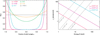 |
Fig. 1. Left: different injected electron anisotropy at the loop apex using S(μ) (Eq. (11)). Small Δμ produces beamed distributions while large Δμ produces isotropic distributions. Right: turbulent scattering mean free path λs versus electron energy E using Eq. (7) and using λs, 0 = 2 × 10⁷, 2 × 10⁸ and 2 × 109 cm. Turbulent scattering quickly isotropises higher energy electrons. The mean free path λs is also compared with the collisional mean free path (using λ = v4/Γ; grey dashed and dotted lines) for three different densities of n = 1 × 1010 cm−3, n = 1 × 1011 cm−3 and n = 1 × 1012 cm−3. |
2.2. Non-collisional scattering
We also study how non-collisional transport effects such as turbulent scattering change the electron distribution and the resulting X-ray polarization. Other non-collisional effects can change the electron properties, such as beam-driven Langmuir wave turbulence (Hannah et al. 2009), electron re-acceleration (Brown et al. 2009) and/or beam-driven return current (Knight & Sturrock 1977; Emslie 1980; Zharkova & Gordovskyy 2006; Alaoui & Holman 2017), but studying these processes is beyond the scope of the paper.
Here we use an isotropic turbulent scattering approximation2 (e.g. Schlickeiser 1989) where the turbulent scattering diffusion coefficient  is related to the turbulent scattering mean free path λs [cm] and electron velocity v [cm s−1] using
 (4)
(4)
Using the standard quasilinear theory for slab turbulence (Jokipii 1966; Kennel & Petschek 1966; Skilling 1975; Lee 1982; Kontar et al. 2014), λs can be related to the level of turbulent magnetic field fluctuations  resonant with electrons of velocity v by
 (5)
(5)
where Ωce = eB/mc is the electron gyrofrequency [Hz], B is the magnetic field strength [G] and c is the speed of light [cm s−1]. Using for example, E = 25 keV and B = 300 G,  corresponds to 2 × 10⁷ [cm] ≤ λs ≤ 2 × 10⁹ [cm].
In simulations where we investigate the role of non-collisional turbulent scattering, the governing Fokker-Planck equation becomes
![Mathematical equation: $$ \begin{aligned}&\mu \frac{\partial F}{\partial z} = \Gamma m_{\rm e}^2 \;\frac{\partial }{\partial E} \left[ G (u[E] ) \frac{\partial F}{\partial E} + \frac{G (u[E] )}{E} \left( \frac{E}{k_{\rm B }T}-1 \right)F \right]\nonumber \\&\qquad \quad + \frac{\Gamma m_{\rm e}^2}{4E^2} \; \frac{\partial }{\partial \mu } \left[ (1-\mu ^{2}) \biggl ( \mathrm{erf} (u[E] ) - G (u[E] ) \biggr ) \frac{\partial F}{\partial \mu } \right]\nonumber \\&\qquad \quad + \frac{1}{2\lambda _{\rm s}(E)}\frac{\partial }{\partial \mu }\left[(1-\mu ^{2}) \frac{\partial F}{\partial \mu } \right] + S(E,z,\mu ). \end{aligned} $$](/articles/aa/full_html/2020/10/aa38626-20/aa38626-20-eq11.gif) (6)
(6)
For the majority of coronal flare conditions and electron energies, non-collisional turbulent scattering operates on timescales shorter than collisional scattering and can produce greater isotropy and trapping amongst higher energy electrons (see Fig. 1, right panel). By combining X-ray imaging spectroscopy and radio observations of the gyrosynchrotron radiation, Musset et al. (2018) find empirically that the scattering mean free path is
![Mathematical equation: $$ \begin{aligned} \lambda _{\rm s}=\lambda _{\mathrm{s},0} \mathrm{[cm]} \left(\frac{25}{E \mathrm{[keV]}}\right), \end{aligned} $$](/articles/aa/full_html/2020/10/aa38626-20/aa38626-20-eq12.gif) (7)
(7)
where λs, 0 = 2 × 108 cm. In Sect. 4, we use λs, 0 = 2 × 108 cm and λs, 0 = 2 × 109 cm.
In this model higher energy electrons have a smaller turbulent mean free path than lower energy electrons. The model of Musset et al. (2018) is suitable for the purposes of the paper and while it is based upon the observation of a single flare and has large uncertainties, it clearly shows that the mean free path of higher energy electrons (from microwave observations) is smaller than the mean free path of lower energy electrons (from X-ray observations).
Following Jeffrey et al. (2014), and re-writting Eq. (6) as a Kolmogorov forward equation (Kolmogorov 1931), Eq. (6) can be converted to a set of time-independent stochastic differential equations (SDEs) (e.g. Gardiner 1986; Strauss & Effenberger 2017) that describe the evolution of z, E, and μ in Itô calculus:
 (8)
(8)
 (9)
(9)
![Mathematical equation: $$ \begin{aligned}&\mu _{j+1}=\mu _{j}-\left[\frac{\Gamma m_{\rm e}^{2} \biggl ( \mathrm{erf}(u_{j})-G(u_{j}) \biggr ) }{2 E_{j}^{2}} \,\, \mu _{j} + \frac{\mu _{j}}{\lambda _{\rm s}(E_{j})}\right] \, \Delta s \nonumber \\&\qquad \,\, +\sqrt{\left[\frac{ (1-\mu _{j}^{2}) \, \Gamma m_{\rm e}^{2} \, \biggl ( \mathrm{erf}(u_{j})-G(u_{j}) \biggr ) }{2 E_{j}^{2}} + \frac{\left(1-\mu _{j}^{2}\right)}{\lambda _{\rm s}(E_{j})}\right]\, \Delta s} \, \, W_\mu . \end{aligned} $$](/articles/aa/full_html/2020/10/aa38626-20/aa38626-20-eq15.gif) (10)
(10)
We note that Δs [cm] is the step size along the particle path, and Wμ, WE are random numbers drawn from Gaussian distributions with zero mean and a unit variance representing the corresponding Wiener processes (e.g. Gardiner 1986). A simulation step size of Δs = 105 cm is used in all simulations, and E, μ and z are updated at each step j. A step size of Δs = 105 cm is approximately two orders of magnitude smaller than the thermal collisional length in a dense (n = 1011 cm−3) plasma with T ≥ 10 MK (or the collisional length of an electron with an energy of 1 keV or greater, in a cold plasma). The derivation of Eq. (6) and a detailed description of the simulations can be found in Jeffrey et al. (2014).
Equation (6) (and Eqs. (9) and (10)) diverge as E → 0, and as discussed in Jeffrey et al. (2014), the deterministic equation ![Mathematical equation: $ E_{j+1}=\left[E_{j}^{3/2} + \frac{3\Gamma m_{\mathrm{e}}^{2}}{2\sqrt{\pi k_{\mathrm{B}}T}}\Delta s \right]^{2/3} $](/articles/aa/full_html/2020/10/aa38626-20/aa38626-20-eq16.gif) must be used for low energies where Ej ≤ Elow using
must be used for low energies where Ej ≤ Elow using ![Mathematical equation: $ E_{\mathrm{low}}=\left[\frac{3\Gamma m_{\mathrm{e}}^{2}}{2\sqrt{\pi k_{\mathrm{B}} T}} \Delta s\right]^{2/3} $](/articles/aa/full_html/2020/10/aa38626-20/aa38626-20-eq17.gif) – see Jeffrey et al. (2014), following Lemons et al. (2009). For such low energy thermal electrons, μj + 1 can be drawn from an isotropic distribution μ ∈ [ − 1, +1].
– see Jeffrey et al. (2014), following Lemons et al. (2009). For such low energy thermal electrons, μj + 1 can be drawn from an isotropic distribution μ ∈ [ − 1, +1].
Once the electron transport simulations are finished, we also include an additional background coronal thermal component with temperature T and a chosen EM = n2V that is dominant at lower X-ray energies between ≈1−25 keV, and where V is the volume of this source. Although it is possible that the thermal component can produce a small detectable polarization of a few percent (Emslie & Brown 1980), we assume that the coronal Maxwellian source is isotropic and hence, produces completely unpolarized X-ray emission in all the simulations shown here.
2.3. Electron input anisotropy and other injection properties
The initial electron anisotropy is chosen using
 (11)
(11)
where Δμ controls the electron directivity. As Δμ → 0 the distribution is completely beamed, with half directed along one loop leg (μ = −1) and half along the other (μ = +1), and as Δμ → ∞, the electron distribution becomes isotropic (see the left panel of Fig. 1).
In many of the simulation runs shown in Sect. 4, the electron directivity is beamed. Since the directivity is unknown, a beamed distribution is used so that differences in the studied parameters are clearly seen and understood.
For most of the simulations shown here, we input sensible flaring parameters: a simple power law distribution in energy (E−δ) with a spectral index of δ = 5, a low energy cutoff of Ec = 20 keV and an acceleration rate of Ṅ = 7 × 1035 electrons s−1 and in space, we input a Gaussian at the loop apex with a standard deviation of 1″.
2.4. Creation of the X-ray distribution
The electron flux spectrum is calculated and it is converted to a photon spectrum using the full angle-dependent polarization bremsstrahlung cross section as described in Emslie et al. (2008) and Jeffrey & Kontar (2011) and using the cross-section shown in Gluckstern & Hull (1953) and Haug (1972) given by
 (12)
(12)
 (13)
(13)
and
 (14)
(14)
where ϵ is the X-ray photon energy and σ⊥(E, ϵ, Θ) and σ∥(E, ϵ, Θ) are the perpendicular and parallel components of the bremsstrahlung cross-section. Subscripts I, Q, U denote the cross section used for the total X-ray flux (I) and linear polarization components (Q, U) respectively, and
 (15)
(15)
relates θ the photon emission angle measured from the local solar vertical, β the electron pitch-angle (e.g. the angle between the electron velocity and the magnetic field) and Φ the electron azimuthal angle measured in the plane perpendicular to the local solar vertical.
Using the above cross sections the resulting photon flux I and each specific linear polarization state Q and U can be written as:
 (16)
(16)
 (17)
(17)
 (18)
(18)
2.5. X-ray transport effects and determining the polarization observables
Depending on the directivity, some fraction of the emitted X-rays are transported to the photosphere. Here Compton backscattering will change the properties of these X-rays before their escape towards the observer. This is known as the X-ray albedo component (e.g. Tomblin 1972; Santangelo et al. 1973; Bai & Ramaty 1978) and all X-ray observables including the flux and polarization spectra are altered by this albedo component. Hence, we employ the code of Jeffrey & Kontar (2011) to create the X-ray albedo component for all simulation runs. A full discussion regarding this code can be found in Jeffrey & Kontar (2011).
Once the X-ray albedo component has been included, two polarization observables, the degree of polarization (DOP) and polarization angle Ψ can be calculated using
 (19)
(19)
and
 (20)
(20)
The negatives in Eq. (20) ensure that Ψ = 0° corresponds to a dominant polarization direction parallel to the local solar radial direction (negative DOP) and Ψ = 90° corresponds to a dominant polarization direction perpendicular to the local solar radial direction (positive DOP). We note that high energy electrons (MeV) can produce spatially integrated Ψ = 90° and thus positive DOP, due to electrons with higher energies scattering through larger angles, providing a useful diagnostic for the presence of MeV electrons. Moreover, Emslie et al. (2008) showed that values of spatially integrated Ψ other than 0° or 90° are possible when the tilt of the flare loop moves away from the local vertical direction (loop tilt τ). Finally, we note that in the case of spatially resolved observations, the angle of polarization Ψ can have values other than Ψ = 0° or Ψ = 90° due to the Compton scattered albedo component as shown in Jeffrey & Kontar (2011), providing a detailed probe of electron directivity in the chromosphere.
Here we only study spatially integrated X-ray data for relatively low electron energies < 300 keV and for flare loops aligned along the local solar vertical. Hence Ψ = 0° and DOP is negative for all simulations. Therefore, since Ψ and the sign of DOP do not change, we only show the DOP results (and as a percentage only).
3. Prospective X-ray polarization instrumentation
Instrumentation to specifically detect solar flare HXR polarization are currently being researched and developed and three such instruments are summarised here. Currently, the most advanced concept is the Gamma-Ray Imager/Polarimeter for Solar flares (GRIPS, Duncan et al. (2016)). GRIPS is a balloon-borne telescope designed to study solar-flare particle acceleration and transport. It has already flown once in Antarctica in January 2016, and will be re-proposed for flight during the next Solar Maximum. GRIPS can do imaging spectro-polarimetry of solar flares in the ∼150 keV to ∼10 MeV range, with a spectral resolution of a few keV, and an angular resolution of ∼12.5″. GRIPS’s key technological improvements over the current solar state of the art at HXR/gamma-ray energies, RHESSI, include 3D position-sensitive germanium detectors (3D-GeDs) and a single-grid modulation collimator, the multi-pitch rotating modulator (MPRM). Focusing optics or Compton imaging techniques are not adequate for separating magnetic loop footpoint emissions in flares over the GRIPS energy band, and indirect imaging methods must be employed. The GRIPS MPRM covers 13 spatial scales from 12.5″ to 162″. For comparison, RHESSI could only image gamma-ray emissions at two spatial scales (35″ and 183″). For photons that Compton scatter, usually ≳150 keV, the energy deposition sites can be tracked, providing polarization measurements as well as enhanced background reduction through Compton imaging. The nominal GRIPS balloon payload has a minimum detectable polarization (MDP) signal of ∼3% in the 150–650 keV band for 2002-July-23 X-flare, while a spacecraft version will likely be closer to ∼1%. While we plan to discuss the spatially resolved observations of GRIPS in another study, here we concentrate on the usefulness of spatially integrated observations of the polarization (DOP) spectrum at lower energies.
In the HXR (∼10–100 keV) regime, the proposed Sapphire (Solar Polarimeter for Hard X-rays, Saint-Hilaire et al. 2019) concept aims to do spatially-integrated spectro-polarimetry of solar flares from CubeSat platforms. A single Sapphire module is expected to be able to detected polarization in the ∼1.5% threshold (≥20 keV, 3-sigma) for a similar flare. Sapphire modules are designed to be stackable, with the decrease (improvement) in MDP for N modules roughly behaving as  .
.
Other proposed missions include the Japanese PhoENiX mission (Physics of Energetic and Non-thermal plasmas in the X (= magnetic reconnection) region, Narukage 2019) which will have an X-ray spectro-polarimeter on board measuring over an energy range of 60–300 keV (and 20–300 keV for spectroscopy).
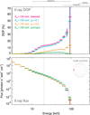 |
Fig. 2. Resulting spatially integrated X-ray DOP and flux spectra for three injected electron distributions with either beamed, Δμ = 0.5, Δμ = 0.1 or isotropic pitch-angle distributions and using the following identical electron properties of: δ = 5, Ec = 20 keV (vertical grey dotted line), EH = 100 keV and Ṅ = 7 × 1035 e s−1, and corona plasma properties of: n = 3 × 1010 cm−3 and T = 20 MK, plotted for a flare located at a heliocentric angle of θ = 60°. All spectra include an albedo component and a coronal background thermal component with EM = n2V = 0.9 × 1048 cm−3, using a chosen V = 1027 cm3. For example error calculations, we use an effective area of 5 cm2 and a time bin of 120 s. No turbulent scattering is present. |
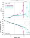 |
Fig. 3. Resulting spatially integrated X-ray DOP and flux spectra for injected electron distributions with different high energy cutoffs of EH = 100 keV, EH = 200 keV and EH = 300 keV. Each use the following identical electron and plasma properties of: δ = 5, Ec = 20 keV (vertical grey dotted line), a beamed distribution and |

4. Results
We investigate how spatially integrated X-ray DOP changes with anisotropy, high energy cutoff and non-collisional turbulent scattering. DOP (and indeed polarization angle) will vary with the flare geometrical properties such as heliocentric angle and the properties of the flare loop such as loop tilt to the local vertical direction, but these properties can always be estimated from flare imaging (see Appendix A, Fig. A.1). In the following sections, all results are shown for a heliocentric angle of 60° and a loop tilt of 0° (the loop apex is parallel to the local vertical direction).
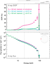 |
Fig. 4. Resulting spatially integrated X-ray DOP and flux spectra for injected beamed electron distributions with EH = 100 keV without turbulent scattering, and with turbulent scattering (using λs, 0 = 2 × 108 cm or λs, 0 = 2 × 109 cm) situated in the coronal loop over a distance of [−10″, +10″] from the loop apex. Each use the following identical electron and plasma properties of: δ = 5, Ec = 20 keV (vertical grey dotted line), a beamed distribution and Ṅ = 7 × 1035 e s−1, and coronal plasma properties of: n = 3 × 1010 cm−3 and T = 20 MK, plotted for a flare located at a heliocentric angle of θ = 60°. All DOP spectra include an albedo component and a coronal thermal component (EM = 0.9 × 1048 cm−3). The results suggest that a lack of coronal turbulent scattering could be detectable from the DOP spectrum. |
4.1. X-ray polarization and electron anisotropy
Traditionally, the prime diagnostic of X-ray polarization is its direct link with electron directivity. Figure 2 shows the spatially integrated DOP (%) versus X-ray energy for four different injected electron anisotropies from completely beamed to isotropic3, for a given set of otherwise identical coronal plasma parameters and electron spectral and spatial parameters. The resulting DOP spectra contains an albedo component and a thermal component as described in Sect. 2. As expected, the DOP at all energies clearly decreases with increasing injected electron isotropy. In Fig. 2, we plot the results for an average coronal number density of n = 3 × 1010 cm−3 and coronal temperature of T = 20 MK. The plasma properties of the corona do change the resulting DOP slightly, particularly at lower energies below 50 keV, however, properties such as the average coronal number density can be estimated from the X-ray flux spectrum and/or EUV spectral observations, and applied to the DOP spectrum.
In Fig. 2, we plot the X-ray flux and DOP over an energy range of ≈3−100 keV, where the flare count rates are highest (most flare spectra are steeply decreasing power laws). As an example in Figs. 2–4, we calculate sensible flux and DOP error values using counts = flux × effective area (A)×time bin (ΔT)×energy bin (ΔE) and assuming that photons = counts. The error on the flux is then calculated as  and the corresponding DOP error as
  . Here we use A = 5 cm2 and Δt = 120 s, with ΔE shown in each figure. We plot the resulting DOP spectra for a flare located at a heliocentric angle of 60° (the DOP should grow as the heliocentric angle approaches the limb).
Comparison of the determined parameters and those input into the simulation.
4.2. X-ray polarization and the high energy cutoff
Another important diagnostic of the acceleration mechanism is the high energy cutoff (the highest energy electrons produced by the acceleration process). The high energy cutoff is also dependent on the spatial extent of the acceleration region and the acceleration time, making it an important modelling constraint. Although the presence of high (MeV) energy electrons might be determinable from microwave observations if present e.g. Melnikov et al. (2002) and Gary et al. (2018), we show that the high energy cutoff changes the trend in the DOP spectra (and also the sign of the polarization angle Ψ for MeV energies as discussed in Jeffrey & Kontar (2011)). We show that the presence of higher energy keV electrons in the distribution can decrease the overall DOP at all observed energies.
In Fig. 3, we plot the resulting DOP spectra from three injected electron distributions with different high energy cutoffs of 100 keV, 200 keV and 300 keV. After 20 keV, we can see that the gradient of the DOP spectrum decreases with an increase in the high energy cutoff EH, producing a flattening and then a decrease in DOP with energy as the high energy cutoff increases to EH = 300 keV, over a typical observed flare energy range of ≈10−100 keV.
This occurs because the resulting X-ray directivity is also dependent on the bremsstrahlung cross section. For example, an 80 keV X-ray is more likely to be emitted by an electron of energy 100 keV than an electron of energy 80 keV (i.e. magnitude of the cross section), with the directivity of the emitted 80 keV X-ray decreased (i.e. the cross section is more isotropic; see Appendix B, Fig. B.2). However, solar flare electron energy spectra are steeply decreasing power laws and to check that the X-ray emission from high energy electrons can indeed contribute enough emission to significantly decrease the X-ray directivity and DOP, two electron distributions with EH = 100 keV and EH = 300 keV, and δ = 5 are compared (see Appendix B, Fig. B.1). By studying the emission from each electron distribution above and below an example energy of 40 keV separately, we see that for X-rays above 25–30 keV, the contribution from higher energy electrons dominates, with this contribution dominating more at lower X-ray energies for higher EH.
This ultimately means that electron distributions with higher electron energies will produce lower energy X-rays with a smaller DOP, even for the same injected beaming. This is an important diagnostic tool that can help to constrain the highest energies in the electron distribution, even when they are completely undetectable by other means. The X-ray DOP spectrum is always a result of both the electron anisotropy and high energy cutoff and both parameters should be determined in tandem.
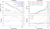 |
Fig. 5. Example of how the X-ray flux and DOP spectra can be used together to estimate the properties of the accelerated electron distribution. Applying the warm target function (f_thick_warm in OSPEX) to the X-ray flux helps to constrain the coronal plasma properties and the following acceleration parameters: low energy cutoff Ec, the spectral index δ and the rate of acceleration Ṅ. Ignoring any other transport mechanisms, and once constrained, the resulting X-ray DOP spectra should only be dependent upon the high energy cutoff EH and acceleration anisotropy Δμ, and turbulent scattering (using λs, 0), if present. Top panels: (left) the “flux data” (black) and the resulting f_vth+f_thick_warm fits to the X-ray flux spectrum (red and green respectively, this also contains an albedo component not shown), and (right) the “DOP data” (black) and four simulation runs using the constrained properties from the X-ray flux spectra and the values of EH, Δμ and λs, 0 shown. Bottom panels: residuals and resulting reduced χ2 for each fit. Both the X-ray flux and DOP are fitted between 3 and 90 keV (grey dash-dot line). |
4.3. Transport versus injection properties
Other transport effects such as turbulent scattering also alter the properties of the electron distribution, including the anisotropy and hence the X-ray polarization. An estimation of the plasma properties from the X-ray flux spectrum, imaging and EUV observations can determine the effects due to collisions, however, constraining the presence and properties of additional non-collisional transport effects outside of the acceleration region can be challenging in the majority of flares. Since DOP is sensitive to changes in anisotropy, we test if the DOP spectra can be used to separate acceleration isotropy with isotropy produced by additional transport processes in the corona outside of the acceleration region.
In Fig. 4, as one example, we plot the DOP versus energy for three identical beamed electron distributions with EH = 100 keV, with no coronal turbulence and with turbulence (λs, 0 = 2 × 108 cm and λs, 0 = 2 × 109 cm) situated in the coronal loop over a distance of [−10″, +10″] from the loop apex. As expected, the presence of turbulence in the corona increases the electron isotropy and hence, reduces the DOP at all energies. Even very beamed distributions produce low levels of DOP when turbulent scattering is present, as shown in Fig. 4.
Using DOP only, it is difficult to distinguish between an initially isotropic electron distribution and the presence of strong turbulence in the corona outside of the acceleration region, although it is suggestive that if strong turbulence is present in the corona then it is also highly likely to be present in the coronal acceleration region. Turbulence greatly affects higher energy electrons and isotropises them quickly leading to low DOP at all energies. The results indicate that a lack of turbulence in the flaring corona can be determined from the DOP spectrum. Figure 4 also shows interesting differences between strong and milder turbulent scattering (i.e. slightly greater DOP at large energies from stronger turbulent scattering) that will be investigated further for different turbulent conditions beyond the scope of this study.
4.4. Extracting parameters from a combined X-ray flux and DOP spectral analysis
The above results show that X-ray polarization is dependent on several important electron acceleration properties and the coronal plasma properties. Moreover, this shows that the DOP spectrum is a powerful diagnostic tool, particularly when used alongside the X-ray flux spectrum.
As a preliminary demonstration of how we could extract vital acceleration parameters from combined X-ray flux and DOP spectra together, we simulate a flare at a heliocentric angle of 60° with certain accelerated electron and background coronal properties (see Table 1), producing the resulting X-ray flux and DOP spectra shown in Fig. 5. To each spectrum, we add noise and we assume a spacecraft background level of 10−2 photons s−1 cm−2 keV−1 at all energies. We now treat the outputs as observational data with unknown properties. Firstly, to the X-ray flux spectrum, we apply the Solar Software (SSW)/OSPEX fitting function routines (as with real flare data). We fitted the X-ray flux spectrum with an isothermal function (f_vth in OSPEX) and warm-target fitting function (f_thick_warm in OSPEX), using the steps described in Kontar et al. (2019). In this fit, as is usual with data, we set EH = 200 keV, a value above the highest energy used in the fitting (90 keV). From fitting, we determine the following accelerated electron parameters: Ṅ = (7.19 ± 0.58) × 1035 e s−1, δ = −4.93 ± 0.39, Ec = 26.6 ± 1.7 keV, and the surrounding coronal plasma parameters of T = 23.3 ± 0.1 MK, EM = (0.24 ± 0.02)×1049 cm−3 and  cm−3 where V is the volume of the hot plasma, assuming a sensible flare volume of V ≈ 1 × 1027 cm−3 and loop length L = 24″, as shown in Table 1. Once these parameters are constrained, we can fix them in the simulation. Then, the only unknowns are EH, Δμ and any coronal loop turbulence described here using λs, 0. Using different simulation runs, we can constrain and determine these parameters by comparison with the observed flare X-ray DOP spectrum. In Fig. 5, four such runs are shown and compared with the DOP spectrum; the runs use different anisotropies, high energy cutoffs and one with turbulent scattering filling the entire corona loop. The residuals and goodness of fit χ2 (calculated as the sum of the residuals divided by the number of fitted energy bins) of each resulting simulation “model” are also shown as an example of how observations and models can be compared.
In Table 1, we show all the determined electron and plasma parameters, the method used to obtain each parameter and compare with the actual parameters that were used in the original ‘data’ simulation. Using X-ray flux and X-ray DOP observations together provides us with a fuller understanding of the solar flare acceleration mechanism. Our analysis shows that current modelling is capable of producing estimates of EH and Δμ, and determining whether turbulence exists in the corona. It will be possible to determine the uncertainties on these variables using many simulation runs and a full Monte Carlo parameter space analysis. However, this full uncertainty analysis is beyond the scope of the current work, since the aim here is to demonstrate how the DOP spectrum can be used as a powerful diagnostic tool alongside the X-ray flux spectrum if the data becomes available.
The DOP is also sensitive to other electron acceleration parameters such as e.g. spectral index and breaks in the spectrum. However, as shown these parameters can be constrained from the X-ray flux spectrum before analysing the DOP spectrum, showing the importance of studying the X-ray flux and DOP spectra in tandem.
5. Summary
X-ray polarimetry is a vital tool for constraining the solar flare acceleration mechanism especially when used alongside the X-ray flux spectrum. The X-ray DOP spectrum is highly sensitive to currently unknown properties such as the accelerated electron pitch-angle distribution, highest energy accelerated electrons and the presence of turbulence in the corona. We have simulation tools available to analyse the X-ray DOP spectrum in detail, if the observations become available and although imaging polarimetry is highly desired, our results show that missions without imaging can also provide strong constraints on electron anisotropy and the high energy cutoff.
In this paper we specifically discussed transport processes that can change the pitch angle distribution of electrons such as Coulomb collisions and turbulent scattering due to magnetic fluctuations but other transport processes may be present. We used a model with a simple homogenous background plasma in the corona since we cannot study the individual plasma properties of each flare. Spatial variations in parameters such as number density along the loop will cause changes in the DOP spectrum. If such changes can be inferred from the data, then they can be incorporated into the model before the inference of acceleration properties.
For this the pitch-angle term in Eq. (1) is multiplied by 2, compared to Jeffrey et al. (2014, 2019).
We use this model for turbulent scattering since the details of scattering in the flaring corona are not well-constrained, i.e. there are many models but few observations.
For comparison, the emitting electron distribution has been forced to be completely isotropic and the DOP spectrum peaking at 2–3% results purely from the backscattered albedo component (e.g. Bai & Ramaty 1978; Jeffrey & Kontar 2011).
Acknowledgments
The development of the electron and photon transport models are part of an international team grant (“Solar flare acceleration signatures and their connection to solar energetic particles” http://www.issibern.ch/teams/solflareconnectsolenerg/) from ISSI Bern, Switzerland. NLSJ acknowledges IDL support provided by the UK Science and Technology Facilities Council (STFC). We thank the anonymous referee for their useful comments that helped to improve the text.
References
- Alaoui, M., & Holman, G. D. 2017, ApJ, 851, 78 [CrossRef] [Google Scholar]
- Aschwanden, M. J., Boerner, P., Ryan, D., et al. 2015, ApJ, 802, 53 [NASA ADS] [CrossRef] [Google Scholar]
- Aschwanden, M. J., Caspi, A., Cohen, C. M. S., et al. 2017, ApJ, 836, 17 [NASA ADS] [CrossRef] [Google Scholar]
- Bai, T., & Ramaty, R. 1978, ApJ, 219, 705 [NASA ADS] [CrossRef] [Google Scholar]
- Benz, A. O. 2017, Liv. Rev. Sol. Phys., 14, 2 [Google Scholar]
- Brown, J. C. 1971, Sol. Phys., 18, 489 [NASA ADS] [CrossRef] [Google Scholar]
- Brown, J. C., Turkmani, R., Kontar, E. P., MacKinnon, A. L., & Vlahos, L. 2009, A&A, 508, 993 [NASA ADS] [CrossRef] [EDP Sciences] [Google Scholar]
- Chen, B., Bastian, T. S., Shen, C., et al. 2015, Science, 350, 1238 [NASA ADS] [CrossRef] [Google Scholar]
- Duncan, N., Saint-Hilaire, P., Shih, A. Y., et al. 2016, Proc. SPIE, 9905, 99052Q [CrossRef] [Google Scholar]
- Emslie, A. G. 1980, ApJ, 235, 1055 [NASA ADS] [CrossRef] [Google Scholar]
- Emslie, A. G., & Brown, J. C. 1980, ApJ, 237, 1015 [NASA ADS] [CrossRef] [Google Scholar]
- Emslie, A. G., Bradsher, H. L., & McConnell, M. L. 2008, ApJ, 674, 570 [NASA ADS] [CrossRef] [Google Scholar]
- Emslie, A. G., Dennis, B. R., Shih, A. Y., et al. 2012, ApJ, 759, 71 [NASA ADS] [CrossRef] [Google Scholar]
- Gardiner, C. W. 1986, Appl. Opt., 25, 3145 [Google Scholar]
- Gary, D. E., Chen, B., Dennis, B. R., et al. 2018, ApJ, 863, 83 [CrossRef] [Google Scholar]
- Gluckstern, R. L., & Hull, M. H. 1953, Phys. Rev., 90, 1030 [NASA ADS] [CrossRef] [Google Scholar]
- Hannah, I. G., Kontar, E. P., & Sirenko, O. K. 2009, ApJ, 707, L45 [NASA ADS] [CrossRef] [Google Scholar]
- Haug, E. 1972, Sol. Phys., 25, 425 [NASA ADS] [CrossRef] [Google Scholar]
- Holman, G. D., Aschwanden, M. J., Aurass, H., et al. 2011, Space Sci. Rev., 159, 107 [NASA ADS] [CrossRef] [Google Scholar]
- Jeffrey, N. L. S. 2014, PhD Thesis, University of Glasgow, UK [Google Scholar]
- Jeffrey, N. L. S., & Kontar, E. P. 2011, A&A, 536, A93 [NASA ADS] [CrossRef] [EDP Sciences] [Google Scholar]
- Jeffrey, N. L. S., Kontar, E. P., Bian, N. H., & Emslie, A. G. 2014, ApJ, 787, 86 [NASA ADS] [CrossRef] [Google Scholar]
- Jeffrey, N. L. S., Kontar, E. P., & Fletcher, L. 2019, ApJ, 880, 136 [CrossRef] [Google Scholar]
- Jokipii, J. R. 1966, ApJ, 146, 480 [Google Scholar]
- Karney, C. 1986, Comput. Phys. Rep., 4, 183 [Google Scholar]
- Kennel, C. F., & Petschek, H. E. 1966, J. Geophys. Res., 71, 1 [NASA ADS] [CrossRef] [Google Scholar]
- Knight, J. W., & Sturrock, P. A. 1977, ApJ, 218, 306 [NASA ADS] [CrossRef] [Google Scholar]
- Kolmogorov, A. 1931, Math. Ann., 104, 415 [CrossRef] [MathSciNet] [Google Scholar]
- Kontar, E. P., Brown, J. C., Emslie, A. G., et al. 2011, Space Sci. Rev., 159, 301 [NASA ADS] [CrossRef] [Google Scholar]
- Kontar, E. P., Bian, N. H., Emslie, A. G., & Vilmer, N. 2014, ApJ, 780, 176 [NASA ADS] [CrossRef] [Google Scholar]
- Kontar, E. P., Jeffrey, N. L. S., Emslie, A. G., & Bian, N. H. 2015, ApJ, 809, 35 [NASA ADS] [CrossRef] [Google Scholar]
- Kontar, E. P., Perez, J. E., Harra, L. K., et al. 2017, Phys. Rev. Lett., 118, 155101 [NASA ADS] [CrossRef] [Google Scholar]
- Kontar, E. P., Jeffrey, N. L. S., & Emslie, A. G. 2019, ApJ, 871, 225 [CrossRef] [Google Scholar]
- Larosa, T. N., & Moore, R. L. 1993, ApJ, 418, 912 [NASA ADS] [CrossRef] [Google Scholar]
- Leach, J., & Petrosian, V. 1983, ApJ, 269, 715 [NASA ADS] [CrossRef] [Google Scholar]
- Lee, M. A. 1982, J. Geophys. Res., 87, 5063 [NASA ADS] [CrossRef] [Google Scholar]
- Lemons, D. S., Winske, D., Daughton, W., & Albright, B. 2009, J. Comput. Phys., 228, 1391 [CrossRef] [Google Scholar]
- Lifshitz, E. M., & Pitaevskii, L. P. 1981, Physical Kinetics (Course of theoretical physics) (Oxford: Pergamon Press), 1981 [Google Scholar]
- Lin, R. P., Dennis, B. R., Hurford, G. J., et al. 2002, Sol. Phys., 210, 3 [Google Scholar]
- Mann, G., Warmuth, A., & Aurass, H. 2009, A&A, 494, 669 [NASA ADS] [CrossRef] [EDP Sciences] [Google Scholar]
- McConnell, M. L., Ryan, J. M., Smith, D. M., Lin, R. P., & Emslie, A. G. 2002, Sol. Phys., 210, 125 [NASA ADS] [CrossRef] [Google Scholar]
- Melnikov, V. F., Shibasaki, K., & Reznikova, V. E. 2002, ApJ, 580, L185 [NASA ADS] [CrossRef] [Google Scholar]
- Musset, S., Kontar, E. P., & Vilmer, N. 2018, A&A, 610, A6 [NASA ADS] [CrossRef] [EDP Sciences] [Google Scholar]
- Narukage, N. 2019, Am. Astron. Soc. Meeting Abstr., 234, 126.03 [Google Scholar]
- Parker, E. N. 1957, J. Geophys. Res., 62, 509 [Google Scholar]
- Petrosian, V. 2012, Space Sci. Rev., 173, 535 [NASA ADS] [CrossRef] [Google Scholar]
- Priest, E., & Forbes, T. 2000, Magnetic Reconnection (Cambridge, UK: Cambridge University Press) [CrossRef] [Google Scholar]
- Saint-Hilaire, P., Jeffrey, N. L. S., Martinez Oliveros, J. C., et al. 2019, AGU Fall Meeting Abstracts, 2019 SH31C-3310 [Google Scholar]
- Santangelo, N., Horstman, H., & Horstman-Moretti, E. 1973, Sol. Phys., 29, 143 [NASA ADS] [CrossRef] [Google Scholar]
- Schlickeiser, R. 1989, ApJ, 336, 243 [NASA ADS] [CrossRef] [Google Scholar]
- Skilling, J. 1975, MNRAS, 172, 557 [NASA ADS] [CrossRef] [Google Scholar]
- Strauss, R. D. T., & Effenberger, F. 2017, Space Sci. Rev., 212, 151 [NASA ADS] [CrossRef] [Google Scholar]
- Sweet, P. A. 1958, IAU Symp., 6, 123 [Google Scholar]
- Tomblin, F. F. 1972, ApJ, 171, 377 [NASA ADS] [CrossRef] [Google Scholar]
- Vlahos, L., Pisokas, T., Isliker, H., Tsiolis, V., & Anastasiadis, A. 2016, ApJ, 827, L3 [NASA ADS] [CrossRef] [Google Scholar]
- Warmuth, A., & Mann, G. 2016, A&A, 588, A116 [NASA ADS] [CrossRef] [EDP Sciences] [Google Scholar]
- Zharkova, V. V., & Gordovskyy, M. 2006, ApJ, 651, 553 [NASA ADS] [CrossRef] [Google Scholar]
Appendix A: Change in DOP versus energy with heliocentric angle and loop tilt
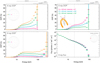 |
Fig. A.1. Left: change in spatially integrated X-ray DOP versus energy for four different heliocentric angles of 20°, 40°, 60° and 80° (as shown by the coloured dots). In this example, all electron distributions are beamed with EH = 100 keV (top panel) and EH = 300 keV (bottom panel). Right: change in spatially integrated X-ray DOP and flux versus energy for different loop tilts of τ = 0°, 25°, 45° (the apex of the loop is tilted by an angle relative to the local vertical – see small cartoon). Each (left and right) uses the following identical electron properties of: δ = 5, Ec = 20 keV (grey dotted line), and Ṅ = 7 × 1035 e s−1, and corona plasma properties of: n = 3 × 1010 cm−3 and T = 20 MK. All spectra include an albedo component and a coronal background thermal component (EM = 0.9 × 1048 cm−3). |
The spatially integrated DOP changes with both flare location on the solar disk (heliocentric angle) and with loop tilt (how the loop apex is tilted with respect to the local vertical; the polarization angle also changes with loop tilt, Emslie et al. 2008). However, both the heliocentric angle and loop tilt can be estimated from imaging the flare in different wavelengths (e.g. EUV). We show some examples of how DOP changes with heliocentric angle and loop tilt in Fig. A.1.
Appendix B: Bremsstrahlung cross section and the contribution from high energy electrons
In Sect. 4.2, we determined that a high energy cutoff leads to lower DOP across all energies and explained that this is due to the production of a more isotropic X-ray distribution when higher energy electrons are present. To confirm this, in Fig. B.1 we plot the resulting X-ray fluxes from electrons of energy E ≤ 40 keV (dashed line) and from electrons of energy E > 40 keV (solid line) separately, but from the same emitting electron distribution. This is shown for an electron distribution with a high energy cutoff of EH = 100 keV (top panel) and EH = 300 keV (middle panel), and a spectral index of δ = 5. The bottom panel of Fig. B.1 shows the X-ray contribution ratio (defined as the X-ray emission from E > 40 keV divided by the X-ray emission from E ≤ 40 keV) versus energy up to 40 keV, for electron distributions with EH = 100 keV and EH = 300 keV respectively.
Although, the contribution will vary with other properties such as spectral index δ, we can see that for both EH = 100 keV and EH = 300 keV, the X-ray contribution from higher energy electrons (E > 40 keV) dominates from above 25 keV (EH = 300 keV) and above 30 keV (EH = 100 keV). Therefore, it shows that the bulk of the X-rays > 25 keV (EH = 300 keV) and > 35 keV (EH = 100 keV) will be dominated by a closer to isotropic X-ray distribution produced by electrons with E > 40 keV (Fig. B.2).
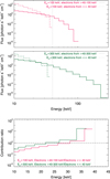 |
Fig. B.1. Resulting X-ray fluxes from electrons of energy E ≤ 40 keV (dashed line) and from electrons of energy E > 40 keV (solid line) separately, for two different high energy cutoff of EH = 100 keV (top) and EH = 300 keV (middle). Bottom: X-ray contribution ratio (the X-ray emission from E > 40 keV divided by the X-ray emission from E ≤ 40 keV) versus energy up to 40 keV (vertical grey dotted line), for electron distributions with EH = 100 keV and EH = 300 keV. The horizontal black dashed-dot line denotes a ratio of 1. |
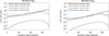 |
Fig. B.2. Total bremsstrahlung cross section (σI) for the emission of a 40 keV X-ray by electrons of different of energies 40, 50, 100 and 300 keV (left) and for the emission of an 80 keV X-ray by electrons of different of energies 80, 90, 100 and 300 keV. |
All Tables
All Figures
|
Fig. 1. Left: different injected electron anisotropy at the loop apex using S(μ) (Eq. (11)). Small Δμ produces beamed distributions while large Δμ produces isotropic distributions. Right: turbulent scattering mean free path λs versus electron energy E using Eq. (7) and using λs, 0 = 2 × 10⁷, 2 × 10⁸ and 2 × 109 cm. Turbulent scattering quickly isotropises higher energy electrons. The mean free path λs is also compared with the collisional mean free path (using λ = v4/Γ; grey dashed and dotted lines) for three different densities of n = 1 × 1010 cm−3, n = 1 × 1011 cm−3 and n = 1 × 1012 cm−3. |
| In the text | |
|
Fig. 2. Resulting spatially integrated X-ray DOP and flux spectra for three injected electron distributions with either beamed, Δμ = 0.5, Δμ = 0.1 or isotropic pitch-angle distributions and using the following identical electron properties of: δ = 5, Ec = 20 keV (vertical grey dotted line), EH = 100 keV and Ṅ = 7 × 1035 e s−1, and corona plasma properties of: n = 3 × 1010 cm−3 and T = 20 MK, plotted for a flare located at a heliocentric angle of θ = 60°. All spectra include an albedo component and a coronal background thermal component with EM = n2V = 0.9 × 1048 cm−3, using a chosen V = 1027 cm3. For example error calculations, we use an effective area of 5 cm2 and a time bin of 120 s. No turbulent scattering is present. |
| In the text | |
|
Fig. 3. Resulting spatially integrated X-ray DOP and flux spectra for injected electron distributions with different high energy cutoffs of EH = 100 keV, EH = 200 keV and EH = 300 keV. Each use the following identical electron and plasma properties of: δ = 5, Ec = 20 keV (vertical grey dotted line), a beamed distribution and |
| In the text | |
|
Fig. 4. Resulting spatially integrated X-ray DOP and flux spectra for injected beamed electron distributions with EH = 100 keV without turbulent scattering, and with turbulent scattering (using λs, 0 = 2 × 108 cm or λs, 0 = 2 × 109 cm) situated in the coronal loop over a distance of [−10″, +10″] from the loop apex. Each use the following identical electron and plasma properties of: δ = 5, Ec = 20 keV (vertical grey dotted line), a beamed distribution and Ṅ = 7 × 1035 e s−1, and coronal plasma properties of: n = 3 × 1010 cm−3 and T = 20 MK, plotted for a flare located at a heliocentric angle of θ = 60°. All DOP spectra include an albedo component and a coronal thermal component (EM = 0.9 × 1048 cm−3). The results suggest that a lack of coronal turbulent scattering could be detectable from the DOP spectrum. |
| In the text | |
|
Fig. 5. Example of how the X-ray flux and DOP spectra can be used together to estimate the properties of the accelerated electron distribution. Applying the warm target function (f_thick_warm in OSPEX) to the X-ray flux helps to constrain the coronal plasma properties and the following acceleration parameters: low energy cutoff Ec, the spectral index δ and the rate of acceleration Ṅ. Ignoring any other transport mechanisms, and once constrained, the resulting X-ray DOP spectra should only be dependent upon the high energy cutoff EH and acceleration anisotropy Δμ, and turbulent scattering (using λs, 0), if present. Top panels: (left) the “flux data” (black) and the resulting f_vth+f_thick_warm fits to the X-ray flux spectrum (red and green respectively, this also contains an albedo component not shown), and (right) the “DOP data” (black) and four simulation runs using the constrained properties from the X-ray flux spectra and the values of EH, Δμ and λs, 0 shown. Bottom panels: residuals and resulting reduced χ2 for each fit. Both the X-ray flux and DOP are fitted between 3 and 90 keV (grey dash-dot line). |
| In the text | |
|
Fig. A.1. Left: change in spatially integrated X-ray DOP versus energy for four different heliocentric angles of 20°, 40°, 60° and 80° (as shown by the coloured dots). In this example, all electron distributions are beamed with EH = 100 keV (top panel) and EH = 300 keV (bottom panel). Right: change in spatially integrated X-ray DOP and flux versus energy for different loop tilts of τ = 0°, 25°, 45° (the apex of the loop is tilted by an angle relative to the local vertical – see small cartoon). Each (left and right) uses the following identical electron properties of: δ = 5, Ec = 20 keV (grey dotted line), and Ṅ = 7 × 1035 e s−1, and corona plasma properties of: n = 3 × 1010 cm−3 and T = 20 MK. All spectra include an albedo component and a coronal background thermal component (EM = 0.9 × 1048 cm−3). |
| In the text | |
|
Fig. B.1. Resulting X-ray fluxes from electrons of energy E ≤ 40 keV (dashed line) and from electrons of energy E > 40 keV (solid line) separately, for two different high energy cutoff of EH = 100 keV (top) and EH = 300 keV (middle). Bottom: X-ray contribution ratio (the X-ray emission from E > 40 keV divided by the X-ray emission from E ≤ 40 keV) versus energy up to 40 keV (vertical grey dotted line), for electron distributions with EH = 100 keV and EH = 300 keV. The horizontal black dashed-dot line denotes a ratio of 1. |
| In the text | |
|
Fig. B.2. Total bremsstrahlung cross section (σI) for the emission of a 40 keV X-ray by electrons of different of energies 40, 50, 100 and 300 keV (left) and for the emission of an 80 keV X-ray by electrons of different of energies 80, 90, 100 and 300 keV. |
| In the text | |
Current usage metrics show cumulative count of Article Views (full-text article views including HTML views, PDF and ePub downloads, according to the available data) and Abstracts Views on Vision4Press platform.
Data correspond to usage on the plateform after 2015. The current usage metrics is available 48-96 hours after online publication and is updated daily on week days.
Initial download of the metrics may take a while.