| Issue |
A&A
Volume 642, October 2020
|
|
|---|---|---|
| Article Number | A92 | |
| Number of page(s) | 8 | |
| Section | Extragalactic astronomy | |
| DOI | https://doi.org/10.1051/0004-6361/202038301 | |
| Published online | 09 October 2020 | |
EeV astrophysical neutrinos from flat spectrum radio quasars
1
INAF – Osservatorio Astronomico di Brera, Via E. Bianchi 46, 23807 Merate, Italy
e-mail: This email address is being protected from spambots. You need JavaScript enabled to view it.
2
DESY, Platanenallee 6, 15738 Zeuthen, Germany
3
Gran Sasso Science Institute (GSSI), Viale F. Crispi 7, 67100 L’Aquila, Italy
4
INFN, Laboratori Nazionali del Gran Sasso (LNGS), 67100 Assergi, L’Aquila, Italy
Received:
30
April
2020
Accepted:
14
June
2020
Abstract
Context. Flat-spectrum radio quasars (FSRQs) are the most powerful blazars in the γ-ray band. Although they are supposed to be good candidates in producing high-energy neutrinos, no secure detection of FSRQs has been obtained to date, except for a possible case of PKS B1424-418.
Aims. In this work, our aim was to compute the expected flux of high-energy neutrinos from FSRQs using standard assumptions for the properties of the radiation fields filling the regions surrounding the central supermassive black hole.
Methods. Starting from the FSRQ spectral sequence, we computed the neutrino spectrum assuming interaction of relativistic protons with internal and external radiation fields. We studied the neutrino spectra resulting from different values of free parameters
Results. The result we obtained is that high-energy neutrinos are naturally expected from FSRQs in the sub-EeV–EeV energy range and not at PeV energies. This justifies the non-observation of neutrinos from FSRQs with the present technology, since only neutrinos below 10 PeV have been observed. We found that for a non-negligible range of the parameters, the cumulative flux from FSRQs is comparable to or even exceeds the expected cosmogenic neutrino flux. This result is intriguing and highlights the importance of disentangling these point-source emissions from the diffuse cosmogenic background.
Key words: neutrinos / BL Lacertae objects: general / radiation mechanisms: non-thermal / astroparticle physics
© ESO 2020
1. Introduction
The extreme phenomenology displayed by active galactic nuclei (AGN) is ultimately associated with the gravitational energy released by gas falling into a supermassive black hole (MBH = 107 − 10 M⊙) residing at the centre of the host galaxies. Active galactic nuclei with relativistic jets, although a minor fraction of the total population, represent the most powerful persistent sources of electromagnetic radiation in the Universe (Blandford et al. 2019). Blazars (Romero et al. 2017) are a subclass of jetted AGNs in which the jet is closely aligned with the line of sight. Under this favourable geometry, the non-thermal emission of the jet is highly amplified by relativistic effects (relativistic beaming). The observed electromagnetic emission of these sources extends over the entire electromagnetic spectrum, and it is characterised by strong variability that can enhance the luminosity by several orders of magnitude during flares. The spectral energy distribution (SED) of blazars – dominated by the non-thermal emission of the relativistic jet – typically shows a double bump shape. The first peak is in the IR-UV band, the maximum of the high-energy one is in the γ-ray band. While the first bump originates from the synchrotron emission of the relativistic electrons in the jet, the physical interpretation of the second peak is still under debate, also in view of the neutrino detection associated with one of these objects (Aartsen et al. 2018). In the pure leptonic model, gamma rays are produced through the inverse Compton scattering by the synchrotron-emitting relativistic electrons. In pure hadronic scenarios, on the other hand, high-energy photons are supposed to be produced through the synchrotron emission of relativistic protons (Aharonian 2000) or the reprocessed radiation produced in photomeson interactions (e.g. Aharonian 2000; Mücke et al. 2003).
Blazars can be divided into two sub-classes: flat-spectrum radio quasars (FSRQs) and BL Lac objects. Their classification is historically based on the width of the emission lines observed in the optical spectra (the traditional division corresponds to an equivalent width of 5 Å). Flat-spectrum radio quasars display broad lines and are generally more powerful than BL Lac, especially in the γ-ray band. On the other hand, BL Lacs, although less powerful, can emit photons at higher energies (up to the multi-TeV band). At present, there is evidence supporting the existence of a continuous trend (or sequence) between the SED of the two sub-classes (see Fossati et al. 1998 and Ghisellini et al. 2017, G17 hereafter).
The IceCube detection of a high-energy neutrino (Eν ∼ 290 TeV) in the direction of a flaring blazar (of which the precise nature is debated, see Padovani et al. 2019), TXS 0506+056, in September 2017 (Aartsen et al. 2018), has lead the community to focus on this class as electromagnetic counterparts of astrophysical neutrinos (Palladino et al. 2019; Murase et al. 2018; Padovani et al. 2016), although many other candidates have been proposed (see Ahlers & Halzen 2014; Mészáros 2017, and Gaisser 2018 for reviews). The production of neutrinos requires the existence of a population of relativistic protons (with energies Ep ≃ 20 × Eν) creating charge pions in collisions with target protons/ions or photons (the latter case is usually referred to as a photomeson reaction). Relativistic protons are thought to be co-accelerated with the electrons, although the details of the mechanisms involved are not completely clear. Considering the low particle density inferred for the relativistic outflows, pion production through the collision with gas is widely considered unlikely (however, see e.g. Sahakyan 2018 for possible scenarios), and therefore neutrino production is expected to proceed mainly through the photomeson channel. This reaction is characterised by a well-defined threshold for energies very close to the one corresponding to the Δ resonance, (pγ → Δ+ followed by the quick decay to pπ0 or nπ+) and this allows one to derive a useful rule of thumb relating the energy of the target photons involved in the reaction, ϵ, and the proton energy, Ep, as Ep ≃ 1.3 × 10¹⁷/ϵ eV (where ϵ is expressed in eV). From this relation, and taking into account the fact that the typical neutrino energy is 1/20 of that of the parent proton, the efficient production of neutrinos with energy in the range 0.1–10 PeV can be linked to target photons in the optical, UV, or soft-X-ray bands.
While they have been suggested to be potential good neutrino emitters (e.g. Murase et al. 2012, Dermer et al. 2014; Kadler et al. 2016), FSRQs are not favoured by current data. In particular, as they are powerful but relatively rare in the sky, one should expect to detect multiplets of neutrino events from single FSRQs already in the current samples (e.g. Murase & Waxman 2016). This rules out the possibility that FSRQs represent the bulk of the sources of the neutrinos detected by IceCube in the 0.1–10 PeV energy range. Interestingly, this conclusion is consistent with the current picture of the structure of FSRQs. In fact, the most intense radiation field expected to interact with relativistic protons in the inner regions of the jet has typical frequencies corresponding to the UV-optical-IR bands, corresponding to relatively large Ep, which in turn implies Eν above the PeV band. In view of the physics programmes of existing and future neutrino telescopes, this expectation deserves careful and quantitative discussion.
In this work, we focus on FSRQs using the state-of-the-art knowledge on their structure and demography to infer their potential neutrino emission. In Sect. 2, we describe the population and the structure of the FSRQs we considered in the work, Sect. 3 describes the calculation of the neutrino emission we used, while Sect. 4 describes the set-up of our models. We report the resulting cumulative predicted spectra in Sect. 5, in which we also compare our results with the most up to date IceCube data, the expected spectra for cosmogenic neutrinos and the sensibility of the future telescope GRAND. Finally, in Sect. 6 we conclude with a discussion.
2. Properties of FSRQs
2.1. Structure
A sketch of the structure of the central regions (distances under a few pc) of FSRQs is reported in Fig. 1. We represent the different regions of interest in our work. Accretion of gas occurs through a standard, optically thick and geometrically thin accretion disc, which is shown in yellow in Fig. 1 (Shakura & Sunyaev 1973). The emission from the disc, peaking in the optical-UV band, irradiates small clouds of gas moving in keplerian orbits around the supermassive black hole (SMBH). The photoionised gasses of the clouds re-emit the intercepted flux in prominent emission lines (with average energy ϵBLR ≃ 10 eV), whose observed profile is broadened by Doppler shift. The (usually assumed shell-like) region filled by these clouds is generally known as the broad-line region (BLR), which is represented in blue in the sketch of Fig. 1. The geometry of the BLR can be probed using the reverberation mapping technique, which allows direct measurements of the distance of the clouds (Kaspi et al. 2007). Beyond the BLR, at typical distances of 1–10 pc, we find a thick structure of dust, traditionally assumed to have a toroidal shape (region 2 of Fig. 1, in purple). Dust grains are powerful absorbers of radiation, and the torus obscures the central regions for observers lying at large angles. Dust heated by the central UV radiation re-emits it as a black-body spectrum at a temperature TIR ≃ 500 − 103 K, peaking in the IR band.
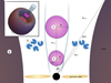 |
Fig. 1. Sketch of geometry we assumed for FSRQs. Region 1 is the emission region containing cosmic rays and photons from the synctrotron emission of electrons. Region 2 and region 3 are the torus and the broad-line region that produce external photon populations. See text for a more detailed description. |
As discussed in Ghisellini & Tavecchio (2009), an approximated estimate of the typical size of the BLR (RBLR) and the torus (Rtorus) can be expressed as a function of the disc luminosity Ld as:
 (1)
(1)
and
 (2)
(2)
These distances are very important since, together with the corresponding luminosities, determine the photon density, a critical parameter for the efficiency of the photopion reactions. We note that, since the radiation energy density is proportional to L/R2, the simple scaling above implies fixed energy densities for all Ld, meaning for all FSRQs.
The jet is launched in the vicinity of the SMBH and it is progressively accelerated and collimated. The physical processes at the base of jet formation and acceleration are still under debate (for a review, see Blandford et al. 2019 or Romero et al. 2017). The scenario outlined by magnetohydrodynamics numerical simulations (e.g. McKinney 2006) describes a jet that starts as a magnetically dominated (Poynting) flow that accelerates progressively converting the magnetic energy flux into kinetic energy flux. The acceleration is relatively low: the flow is expected to reach the final Lorentz factor (where magnetic and kinetic powers are almost in equipartition) around the parsec scale (e.g. Komissarov et al. 2007; Vlahakis 2015 and Nakamura et al. 2018). This is the region generally identified as the “blazar region”, which is the region where the bulk of the radiation observed from blazars is produced.
Jets of FSRQs propagate through the different structures discussed above. In the reference frame of the outflowing plasma, moving with constant bulk Lorentz factor Γ, the energy density of the radiation fields is modified by the relativistic boosting. At distances for which the jet is totally immersed in the (nearly isotropic) radiation field of the BLR or of the torus, the relativistic boosting results in the shift of the frequencies by a factor ≈Γ and the amplification of the energy density by a factor ≈Γ2 with respect to the value measured by an external observer at rest (e.g. Sikora et al. 1994). Although the spectrum emitted by the BLR clouds is rather complex, with the presence of lines and continuum, the boosted emission as observed in the jet rest frame can be well approximated by a peaked, black-body-like spectrum, with the maximum corresponding to the Lyman α line, at an energy  eV Tavecchio & Gabriele (2008). We used this approximation in the calculation of the neutrino spectra.
2.2. Sites of neutrino production
The radiation we observe from FSRQs emerges from an emission region inside the jet. For simplicity, we assume a spherical region, at a distance d from the central SMBH and with a radius R as reported in Fig. 1. We assume a conical jet with semi-aperture angle θj, so that R = dθj. The location of the emission region of an FSRQ is a subject of debate. While standard models assume that the emission mainly occurs at distances lower than RBLR (thus within the dense radiation field of the BLR), the absence of spectral features related to absorption of gamma rays by the UV continuum (e.g. Poutanen & Stern 2010 and Costamante et al. 2018), together with the detection of few FSRQs at TeV energies during flares (e.g. MAGIC Collaboration 2018 or H. E. S. S. Collaboration 2019) indicates that, at least in some cases and/or during high-activity states, the electromagnetic radiation is produced beyond the BLR (e.g. Tavecchio et al. 2011).
In the following, we calculate the neutrino output expected for two cases, notably by assuming the emission region located at a distance d < RBLR and RBLR < d < Rtorus. We distinguish the two scenarios, referring to them as “inside BLR” and “outside BLR”. For the torus, we assume TIR = 500 K.
2.3. Population
To characterise the entire population of FSRQs, we considered the results of Ajello et al. (2012). They offer a parametrisation of the cosmological evolution of FSRQs in terms of their gamma-ray luminosity, redshift, and spectral index of the spectrum between 0.1–100 GeV. In our model, we are only interested to the distribution in redshift and luminosity, therefore the spectral index dependence is disregarded. According to Ajello et al. (2012), these high-luminosity objects are characterised by a positive evolution, and it becomes very strong for the highest luminosity FSRQs, which are distributed as ∼(1 + z)5 for z < 1. These objects are quite rare in the Universe, being characterised by a local density lower than 1 Gpc−3. Moreover, they are very brilliant, varying in the Lγ = 1044 − 1050 erg s−1 range.
In this work, we divided the FSRQ population in five different luminosity bins: from 1044 erg s−1 < Lγ < 1045 erg s−1 to Lγ > 1048 erg s−1. This classification is the same as what was reported in G17, and it serves in the next section to derive the neutrino emission for each FSRQ bin. One possible realisation of the distribution given in Ajello et al. (2012) is shown in the first panel of Fig. 2. In this plot, we show the redshift and the gamma-ray luminosity of 1167 sources1. We also illustrate the separation between resolved and unresolved sources, using a luminosity at Earth of 4 × 10⁻¹² erg cm−2 s−1 as a splitting point, similarly to Palladino et al. (2019). In principle, one can expect that the bolometric (i.e. total) neutrino output is related to the power emitted in the electromagnetic channel. In Murase & Waxman (2016) or Righi et al. (2017), for example, authors assume a linear relation between the γ-ray luminosity and the neutrino one. Here, we find a non-linear relation between the two luminosities because of the models we considered (see Sect. 4).
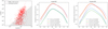 |
Fig. 2. Left panel: cosmological evolution of FSRQs, according to Ajello et al. (2012). Centre and right panels: contribution to the neutrino flux for different parameters we considered in this work. Central and right panels: inside and outside BLR scenarios, respectively. |
The centre and right panels of Fig. 2 show the expected contribution to the neutrino flux for different parameters studied in this work and for the inside and outside BLR scenarios. In all the scenarios, high-luminosity sources contribute most on the expected total neutrino flux from FSRQs.
3. Formalism for neutrino production
To derive the spectrum of the neutrino emission of an FSRQ, we start from the (observed) total, or bolometric, electromagnetic non-thermal luminosity of the jet, Lbol, and the (measured or inferred) disc luminosity, Ld. The latter can be directly translated to the BLR and torus radii through Eq. (1) and (2) above. This uniquely provides the external photon densities as a function of distance along the jet.
The other ingredient we need is the energy distribution of the relativistic cosmic rays (protons, for simplicity). We describe it as a power law with exponential cut off (see below). We normalised the total proton luminosity (i.e. total energy injected into the proton population per unit time) as measured in the jet frame,  (primes denote quantities measured in the jet frame), to the electromagnetic luminosity,
  , meaning we impose
  (we assume this relation as a purely phenomenological description, although it can be justified by simple physical arguments, e.g. Righi et al. 2017). The jet-frame electromagnetic luminosity can be derived from the observed luminosity with
  , where δ is the relativistic Doppler factor that depends on the bulk Lorentz factor Γ and the angle θ between the jet velocity and the line of sight as: δ = [Γ(1 − β cos θ)]−1. Using these relations, we can write:
 (3)
(3)
For a given photomeson efficiency fpγ, the luminosity channelled into neutrinos as measured in the jet frame is proportional to  .
.
To derive the observed electromagnetic luminosity Lbol, we exploited the averaged SED constructed for sources of different γ-ray luminosity by G17. Specifically, G17 considered a sample of 448 FSRQs with known redshift extracted from to the third AGN catalogue detected by Fermi/LAT, 3LAC (Ackermann et al. 2015), grouped them into five bins of gamma-ray luminosity, and for each bin derived an averaged SED using a suitable phenomenological function (see Eq. (11) of G17).
The SED models can be used to derive the average observed bolometric luminosity, Lbol, of the five FSRQ categories. These luminosity bins are representative of the entire population of FSRQs.
We then calculated the neutrino spectrum, adopting the same calculations described in Tavecchio et al. (2014). Here we describe schematically the main assumptions.
The proton population is characterised by a total luminosity in the jet frame,  , and the energy distribution is parametrised by a cut-off energy power law:
 (4)
(4)
The photomeson production efficiency fpγ is calculated as the ratio between the timescales of the adiabatic losses ( , with R as the radius of the jet region) and the cooling rate
  of protons which is given, in the jet frame, by
 (5)
(5)
where nt is the numerical density of the target photons,  and ϵth is the threshold energy of the process. We solved the integral of Eq. (5) using as cross section σpγ and the inelasticity Kpγ provided in Atoyan & Dermer (2003).
The neutrino luminosity  in the jet frame is given by (e.g. Murase et al. 2014):
 (6)
(6)
From the decay of π0 produced in the photomeson reaction, we expect a production of γ-rays with a luminosity  given by:
 (7)
(7)
Finally, we obtained the neutrino luminosity Lν in the observer frame using the Doppler factor δ:
 (8)
(8)
In summary, the free parameters entering in the calculation are: the index and the maximum energy of the proton distribution, n and  , the distance d of the region along the jet where the emission occurs (see Fig. 1), the Lorentz factor Γ, and the Doppler factor δ. To reduce the number of free parameters, we fixed the Lorentz factor Γ = 13 following Ghisellini & Tavecchio (2015) and we assumed δ = Γ (i.e. we fixed the observing angle to 1/Γ).
4. Models
In the following, we consider two different regions inside the jet in which the photopion production occurs. In the first case (inside BLR), we assume that the region is at a distance d < RBLR (where the BLR radius is given by Eq. (1)), and, for precision, we consider that d = RBLR/2. In this case, there are three different photon target populations involved in the pγ reaction: the synchrotron radiation produced inside the jet (assumed to be cospatial with the protons), the radiation from the BLR clouds and the thermal torus radiation. In the second case (outside BLR), we assume the region to be beyond the BLR radius: in this case, there are only the synchrotron radiation and the torus emission as photon targets for the pγ reaction (the BLR radiation is strongly de-amplified in the jet frame, see e.g. Ghisellini & Tavecchio 2009). In this case, we fixed d = RTorus/2 with RTorus given by Eq. (2).
The size RBLR and RTorus (and, therefore, the distance of the emission region in the two scenarios) can be derived from the disc luminosity. We link the disc luminosity to the bolometric non-thermal luminosity of the jet following Ghisellini & Tavecchio (2009) (see also Ghisellini et al. 2014), meaning we assume Ld ≈ Lbol/Γ2.
Assuming a jet semi-aperture angle θj, the radius of the emission region in the inside BLR case is:
 (9)
(9)
where we set the aperture angle to the standard value θj = 1/Γ. For the case outside the BLR, we used the same equation as with RTorus instead of RBLR. This way, we fixed the distance and the size of the emission region, d and R, to Lbol for each bin.
Concerning the maximum energy of the proton distribution,  , we derived it using the condition of equality between cooling and acceleration timescales
  in the jet frame. This condition corresponds to the equilibrium between losses and gains suffered by relativistic protons in the emission region. Losses include photomeson losses with timescale
  , Eq. (5) and adiabatic losses with characteristic timescales:
 (10)
(10)
with R being the radius of the emission region (e.g. Tavecchio & Ghisellini 2015).
The acceleration time can be expressed by:
 (11)
(11)
where  is the proton energy normalised to 1015 eV, B is the magnetic field (for precision, we set B = 5 G), and ηacc is a parameter depending on the details of the acceleration process, and it is estimated to be in the range of 1–100 (e.g. Rieger et al. 2007). For the acceleration time, the relevant parameter is ηacc/B; so our scenario in which we fix the magnetic field but keep ηacc as a free parameter does not affect the calculations.
Figure 3 shows the relevant cooling (blue and orange lines) and acceleration timescales (green lines) for different values of ηacc for an intermediate luminosity bin, 1046 erg s−1 < Lγ < 1047 erg s−1. The intersection between the curve corresponding to the shorter cooling timescale and that for the acceleration timescale fixes the maximum energy attainable by accelerated protons. The vertical black dashed lines indicate the value of  for different values of ηacc. Except for the highest luminosity bins, the cooling is dominated by the adiabatic losses (horizontal orange line).
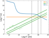 |
Fig. 3. Acceleration and cooling timescales (measured in the jet frame) expected for high-energy protons for an intermediate luminosity bin, 1046 erg s−1 < Lγ < 1047 erg s−1. The blue line shows the photomeson timescale tpγ. Green lines show an estimate of the acceleration timescale for three values of the acceleration efficiency ηacc. The orange horizontal line is the adiabatic timescale. All quantities are expressed in the emission region reference frame. |
This way, the free parameters are now ξ (the parameter linking Lbol with the cosmic ray luminosity, Eq. (3)), n (the index of the proton energy distribution, Eq. (4)), and ηacc (the acceleration efficiency, Eq. (11)). Figure 4 shows how the neutrino spectrum changes for different values of n and ηacc and two luminosity bins of FSRQs (the highest one Lγ > 1048 erg s−1, left panel, and the intermediate one, 1046 erg s−1 < Lγ < 1047 erg s−1, right panel) considering the scenario inside the BLR.
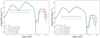 |
Fig. 4. SED and neutrino component for an intermediate bin of FSRQ, 1046 erg s−1 < Lγ < 1047 erg s−1, left panel, and the highest bin Lγ > 1048 erg s−1. Blue line shows the SED derived by G17. Dashed lines correspond to the expected cascade of γ-rays from the π0 decay. In both cases, we report the inside BLR case. |
In Fig. 4, it is clearly visible that the bulk of the neutrino output lies at energies above 1 PeV for the inside the BLR case, and at even larger energies in the other case. This is a combined effect of the threshold and of the spectrum of the target photons. For instance, in the case in which the BLR photon field is dominant, as already remarked, the spectrum in the jet frame can be well approximated with a black-body (BB) shape. Since protons interact mainly with photons at the energy peak of the BB spectrum, we expect that photons with an energy of  eV to be the radiation targets of protons with
  eV. The neutrino produced through photomeson reactions has an energy
  eV, and in the observer frame
  eV. When IR photons from the torus are dominant, the threshold imposes an even larger energy for protons, and in turn for the produced neutrinos. We remark that this result is completely independent on the details of the proton energy distribution (slope, maximum energy), but it is solely the result of the spectral properties of the photon fields.
As discussed in the previous paragraph, photomeson reactions produce neutrinos from the decay of charged pions and γ-rays from the π0 decay. We can derive the spectrum of these photons using Eq. (7). Photons with these energies interacting with low-energy targets are promptly absorbed through the pair production reaction γγ → e+ + e−. The resulting pairs produce high-energy gamma rays through inverse Compton scattering, triggering the development of an electromagnetic cascade inside the emission region. When the energy is degraded below the energy Eτ = 1 for which the optical depth is unity, photons can leave the source. The observed spectrum for saturated cascades is characterised by a universal spectrum with slope ≈1 (i.e. “flat” in the SED representation) extending from a low energy end Emin to Eτ = 1.
The flat cascade component can provide a substantial contribution in the “valley” between the two SED bumps (as extensively discussed for the case of TXS 0506+056, e.g. Ansoldi et al. 2018, Cerruti et al. 2018). The very well-known absence of features associated with cascades in the observed SED of FSRQ (e.g. G17) therefore implies a robust upper limit to the luminosity of the cascade component, and in turn to the neutrino emission.
A detailed calculation of the expected cascade spectrum is beyond our aims. For our purposes, a good approximation of the cascade luminosity can be obtained assuming that the total UHE photon luminosity  injected by the π0 decay (which in the observer frame is
  ) is re-emitted as a flat ∝E−1 component extending from Emin to Eτ = 1. The latter energy can be derived from the condition that the optical depth of the emission region is τ(E) = 1. Emin is more difficult to assess, but the normalisation of the cascade spectrum has a very weak dependence on it. For precision, we assume Emin = 10−3 eV.
As an example, in Fig. 4 we report (horizontal dotted lines) the cascade spectra derived for two luminosity bins and a set of parameters, together with the corresponding SED. For the high-luminosity bin (Lγ > 1048 erg s−1, left panel) the cascade components are relatively more luminous than those corresponding to the lower luminosity bin (1046 erg s−1 < Lγ < 1047 erg s−1, right panel). Therefore, each set of parameters (ηacc, n, ξ) fulfilling the condition that the cascades lie below the valley for the most powerful sources automatically satisfies the constraint for the entire population. We define this as the “low” model.
Another possibility would be to instead adopt different sets of parameters for the different luminosity bins, tuning them so that for each bin the cascade provides the maximum contribution to neutrinos allowed by the SED. Clearly, this case describes the highest total neutrino flux allowed for the entire FSRQ population (“high” case). For simplicity, in this scenario we fixed the power index n = 2 and the acceleration efficiency ηacc = 5. What we obtain is therefore a different value of ξ for each luminosity bin of FSRQs in a range between 9 × 10⁻¹ < ξ < 2 × 10³. This implies that low-power FSRQs should be relatively more efficient than the high-power ones in injecting power on relativistic protons.
To give a comparison between the high and low cases, we plotted the neutrino spectra for all luminosity bins (inside the BLR case) in Fig. 5. In both panels, solid lines are the electromagnetic SED from G17, while dashed lines are the neutrino spectra. In the left panel, the neutrino spectra are obtained using the same values n = 2, ηacc = 5 and ξ = 0.3 far all bins (low case). The right panel instead shows the high scenario with the same values of n and ηacc, but with ξ variable for each bin (as above). It is clear that in this high scenario, the low-luminosity FSRQs are more efficient in producing neutrinos than they are in the low scenario.
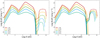 |
Fig. 5. Electromagnetic SED of all categories of FSRQs, solid lines, with the expected neutrino spectra, dashed lines. Left panel: scenario with n = 2, ηacc = 5 and ξ = 0.3. Right panel: maximum scenario with n = 2, ηacc = 5 and ξ variable for each luminosity bin. |
Even if the low case provides a neutrino flux lower than the maximum potential (constrained by the cascade component), it should be considered a relatively optimistic scenario, since we are assuming that protons are accelerated and injected with a relatively large luminosity. Of course, an entire class of models with ξ lower than the minimum assumed are possible, for which the predicted neutrino luminosity would therefore be lower than that derived here.
5. Cumulative neutrino emission
Figures 6 and 7 show the cumulative diffuse neutrino emission from FSRQs for the different scenarios that we consider in this work obtained by convolving the neutrinos spectra with the luminosity functions. In all cases, we compare our results with the IceCube data (blue points for HESE events and light blue band for throughgoing muons, Aartsen et al. 2017), the sensitivity of the future experiment, GRAND (black dashed lines Álvarez-Muñiz et al. 2020), and the expected flux from cosmogenic neutrinos (grey region Alves Batista et al. 2019). Those neutrinos are produced by the interaction of ultra-high-energy cosmic rays, UHECR, interacting with the intergalactic backgrounds including the cosmic microwave background (CMB) and the extragalactic background light (EBL; Berezinsky & Zatsepin 1969). The expected spectrum of the cosmogenic neutrinos displays a tail at low energies due to the interaction of cosmic rays with the UV component of EBL. In fact, the contribution of the interaction of UHECR with EBL is below 1018 eV, while at higher energies, the contribution of UHECR interacting with CMB dominates. In Fig. 6, we report our results considering the inside (left panel) and outside (right panel) scenarios in the low case. We predicted neutrino emission from ten different models (five inside BLR, five outside BLR). All scenarios are compatible with the current limits given by IceCube.
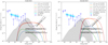 |
Fig. 6. Diffuse neutrino case in the luminosity-dependent case, assuming ηacc = 5 in the left panel and ηacc = 50 in the right panel. The results are compared with the IceCube data (HESE as blue points, throughgoing muons as light blue band) plus the sensitivity of the future experiment GRAND. |
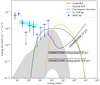 |
Fig. 7. Expected diffuse flux, assuming the maximum ξ for each luminosity bin. |
In the left panel of Fig. 6, in which we consider the emission region inside the BLR, we have two cases in which the maximum plateau of the emission by FSRQs is observable thanks to three years of GRAND observation, and it does not interfere with the peak of the cosmogenic neutrinos (best expectation). Moreover, these two scenarios, in which we have, respectively, n = 2, ξ = 0.3 and ηacc = 1 (red solid line) or ηacc = 5 (yellow solid line), are the only two scenarios among those we considered that provide fluxes clearly detectable with only three years of GRAND observations. For other scenarios (considering softer proton spectra, smaller ξ, or low acceleration efficiency), we predict spectra that are amidst the cosmogenic neutrino region, and more time is needed to clearly identify them.
In the right panel of Fig. 6, we show the outside BLR scenario. In this case, the predicted spectra peak at higher energies than the cosmogenic neutrino emission, because of the low-energy target photon energy from the torus. For this reason, we expect an easy distinction between the cosmogenic component and FSRQ neutrino emission. In addition, we expect an isotropic flux of cosmogenic neutrinos, while we expect neutrinos from FSRQs to point back to the sources.
In Fig. 7, the neutrino emission in the high scenario for both inside (green solid line) and outside (yellow line) cases are shown. In the first case, the cosmogenic neutrino peak is below our prediction, while in the outside case, our spectrum peaks at a higher energy, allowing a possible detection of the cosmogenic neutrinos in the case of the most optimistic scenario. In view of the physics programmes of existing and future neutrino telescopes, this expectation deserves careful and quantitative discussion.
6. Conclusion
Flat-spectrum radio quasars (FSRQs) are the most luminous blazars in the γ-ray band. Their nuclear region, which is naturally rich in photons, is the ideal environment to produce high-energy neutrinos via photohadronic interactions. In this work, we computed the neutrino flux expected from FSRQs using standard assumptions on their structure and a limited selection of the parameters.
In order to estimate the diffuse flux, we used the FSRQ population (i.e. luminosity function and evolution) described by Ajello et al. (2012). We considered two different scenarios, in which neutrinos are produced inside the BLR, with three different photon target populations for the photomeson reaction, or outside the BLR, where only synchrotron and torus radiation contribute to the neutrino production. In both cases, we derive the neutrino emission investigating five different scenarios in which the three main free parameters (the spectral index of relativistic protons n, the acceleration efficiency ηacc, and the parameters ξ that link the bolometric luminosity to the proton luminosity) vary.
Neutrino luminosity is constrained by the photons produced through the decay of π0 that trigger an electromagnetic cascade. The resulting reprocessed photon emission is characterised by a flat spectrum extending over several decades in frequency, contributing especially in the X-ray band, which is the location of the valley between the two SED peaks. The condition that the reprocessed flux lies below the observed (hard) X-ray continuum provides a stringent upper limit to the photomeson reactions. In particular, this provides a constraint on the parameters that we used in our luminosity-independent model. In particular, the highest luminosity bin provides the most stringent constraint.
Then, we considered a more complex model for both inside and outside scenarios, in which all the luminosity bins of FSRQs produce the maximum neutrino emission allowed without exceeding the limit given by the electromagnetic emission. In this model, each luminosity bin had a different value of ξ, which implies that low-power FSRQs are relatively more efficient in injecting power into relativistic protons than the high-power FSRQs.
We remark that a possible dominant component of neutrinos well above 1 PeV is naturally related to the nature of the radiation fields filling the central regions of FSRQ. In fact, due to the threshold that characterises the photopion reaction, only protons with energies above the PeV range (as measured in the jet frame) can interact and produce pions. Lower neutrino energies would require the existence of an unobserved intense field at soft/medium X-ray energies. This prediction is in agreement with the non-detection of FSRQs by the current generation of high-energy neutrino detectors.
We showed the cumulative neutrino flux for the entire population of FSRQs, and, in all scenarios, we considered that the FSRQ could be detectable by future neutrino telescopes in the sub-EeV-EeV energy region. Moreover, in several cases the neutrino flux is higher than the cosmogenic neutrino flux estimates discussed in the literature. Our results are in agreement with the results obtained in Rodrigues et al. (2018), in which the authors identified highly luminous FSRQs as best neutrino emitters among blazar objects.
We would like to note that our results do not completely exclude the possibility that FSRQs provide some contribution to the main signal observed by IceCube. In fact, our analysis is based on the average spectra obtained from the sequence of FSRQ and assumes the structural properties described by the simple relations of Eqs. (1)–(2). Therefore, our calculations should be considered as representative of the average population of an FSRQ and do not describe possible outlier behaviours of the sources. Indeed, in some situations FSRQs could have different values of the various parameter that determine the neutrino emission, such as the Doppler factor or the power-law index. In principle, similar modifications allow some special FSRQs – or most FSRQs in certain special situations or statse – to be more efficient in producing neutrinos in the range ∼100 TeV−1 PeV.
Our results can be easily tested using a future neutrino telescope, since cosmogenic neutrinos are expected to be isotropically distributed, while EeV neutrinos from FSRQs should point back to the source, particularly to FSRQs with a gamma-ray luminosity between 1047 and 1049 erg s−1.
The total number of sources comes directly from the theoretical distribution.
Acknowledgments
We would like to thank F. Halzen for his helpful suggestions, which helped us to improve the discussion of the results. AP has received funding from the European Research Council (ERC) under the European Union’s Horizon 2020 research and innovation programme (Grant No. 646623). CR and FT acknowledge contribution from the grant INAF CTA-SKA, “Probing particle acceleration and gamma-ray propagation with CTA and its precursors” and the INAF Main Stream project “High-energy extragalactic astrophysics: toward the Cherenkov Telescope Array”. This work was partially supported by the research grant number 2017W4HA7S “NAT-NET: Neutrino and Astroparticle Theory Network” under the program PRIN 2017 funded by the Italian Ministero dell’Università e della Ricerca (MUR).
References
- Aartsen, M. G., Ackermann, M., Adams, J., et al. 2017, The IceCube Neutrino Observatory - Contributions to ICRC 2017 Part II: Properties of the Atmospheric and Astrophysical Neutrino Flux [Google Scholar]
- Aartsen, M. G., et al. 2018, Science, 361, eaat1378 [CrossRef] [Google Scholar]
- Ackermann, M., Ajello, M., & Atwood, W. B. 2015, ApJ, 810, 14 [NASA ADS] [CrossRef] [Google Scholar]
- Aharonian, F. A. 2000, New A., 5, 377 [NASA ADS] [CrossRef] [Google Scholar]
- Ahlers, M., & Halzen, F. 2014, Phys. Rev. D, 90, 043005 [NASA ADS] [CrossRef] [Google Scholar]
- Ajello, M., Shaw, M. S., Romani, R. W., et al. 2012, ApJ, 751, 108 [NASA ADS] [CrossRef] [Google Scholar]
- Álvarez-Muñiz, J., Alves Batista, R., & Balagopal, A. 2020, Sci. China. Phys. Mech. Astron., 63, 219501 [Google Scholar]
- Alves Batista, R., de Almeida, R. M., Lago, B., & Kotera, K. 2019, J. Cosmol. Astropart. Phys., 2019, 002 [CrossRef] [Google Scholar]
- Ansoldi, S., Antonelli, L. A., & Arcaro, C. 2018, ApJ, 863, L10 [NASA ADS] [CrossRef] [Google Scholar]
- Atoyan, A. M., & Dermer, C. D. 2003, ApJ, 586, 79 [NASA ADS] [CrossRef] [Google Scholar]
- Berezinsky, V. S., & Zatsepin, G. T. 1969, Phys. Lett., 28B, 423 [NASA ADS] [CrossRef] [Google Scholar]
- Blandford, R., Meier, D., & Readhead, A. 2019, ARA&A, 57, 467 [NASA ADS] [CrossRef] [Google Scholar]
- Cerruti, M., Zech, A., Boisson, C., et al. 2018, in SF2A-2018: Proceedings of the Annual meeting of the French Society of Astronomy and Astrophysics, eds. P. Di Matteo, F. Billebaud, F. Herpin, et al., 235 [Google Scholar]
- Costamante, L., Cutini, S., Tosti, G., Antolini, E., & Tramacere, A. 2018, MNRAS, 477, 4749 [NASA ADS] [CrossRef] [Google Scholar]
- Dermer, C. D., Murase, K., & Inoue, Y. 2014, JHEAp, 3–4, 29 [Google Scholar]
- Fossati, G., Maraschi, L., Celotti, A., Comastri, A., & Ghisellini, G. 1998, MNRAS, 299, 433 [Google Scholar]
- Gaisser, T. K. 2018, ArXiv e-prints [arXiv: 1801.01551] [Google Scholar]
- Ghisellini, G., & Tavecchio, F. 2009, MNRAS, 397, 985 [NASA ADS] [CrossRef] [Google Scholar]
- Ghisellini, G., & Tavecchio, F. 2015, MNRAS, 448, 1060 [NASA ADS] [CrossRef] [Google Scholar]
- Ghisellini, G., Tavecchio, F., Maraschi, L., Celotti, A., & Sbarrato, T. 2014, Nature, 515, 376 [NASA ADS] [CrossRef] [Google Scholar]
- Ghisellini, G., Righi, C., Costamante, L., & Tavecchio, F. 2017, MNRAS, 469, 255 [NASA ADS] [CrossRef] [Google Scholar]
- H. E. S. S. Collaboration (Abdalla, H., et al.) 2019, A&A, 627, A159 [NASA ADS] [CrossRef] [EDP Sciences] [Google Scholar]
- Kadler, M., Krauß, F., Mannheim, K., et al. 2016, Nat. Phys., 12, 807 [Google Scholar]
- Kaspi, S., Brandt, W. N., Maoz, D., et al. 2007, ApJ, 659, 997 [NASA ADS] [CrossRef] [Google Scholar]
- Komissarov, S. S., Barkov, M. V., Vlahakis, N., & Königl, A. 2007, MNRAS, 380, 51 [Google Scholar]
- MAGIC Collaboration (Acciari, V. A., et al.) 2018, A&A, 619, A159 [NASA ADS] [CrossRef] [EDP Sciences] [Google Scholar]
- McKinney, J. C. 2006, MNRAS, 368, 1561 [NASA ADS] [CrossRef] [Google Scholar]
- Mészáros, P. 2017, Ann. Rev. Nucl. Part. Sci., 67, 45 [CrossRef] [Google Scholar]
- Mücke, A., Protheroe, R. J., Engel, R., Rachen, J. P., & Stanev, T. 2003, Astropart. Phys., 18, 593 [Google Scholar]
- Murase, K., & Waxman, E. 2016, Phys. Rev. D, 94, 103006 [NASA ADS] [CrossRef] [Google Scholar]
- Murase, K., Beacom, J. F., & Takami, H. 2012, J. Cosmol. Astropart. Phys., 2012, 030 [CrossRef] [Google Scholar]
- Murase, K., Inoue, Y., & Dermer, C. D. 2014, Phys. Rev. D, 90, 023007 [NASA ADS] [CrossRef] [Google Scholar]
- Murase, K., Oikonomou, F., & Petropoulou, M. 2018, ApJ, 865, 124 [NASA ADS] [CrossRef] [EDP Sciences] [Google Scholar]
- Nakamura, M., Asada, K., & Hada, K. 2018, ApJ, 868, 46 [NASA ADS] [CrossRef] [Google Scholar]
- Padovani, P., Resconi, E., Giommi, P., Arsioli, B., & Chang, Y. L. 2016, MNRAS, 457, 3582 [NASA ADS] [CrossRef] [Google Scholar]
- Padovani, P., Oikonomou, F., Petropoulou, M., Giommi, P., & Resconi, E. 2019, MNRAS, 484, L104 [NASA ADS] [CrossRef] [Google Scholar]
- Palladino, A., Rodrigues, X., Gao, S., & Winter, W. 2019, ApJ, 871, 41 [NASA ADS] [CrossRef] [Google Scholar]
- Poutanen, J., & Stern, B. 2010, ApJ, 717, L118 [Google Scholar]
- Rieger, F. M., Bosch-Ramon, V., & Duffy, P. 2007, Ap&SS, 309, 119 [NASA ADS] [CrossRef] [Google Scholar]
- Righi, C., Tavecchio, F., & Guetta, D. 2017, A&A, 598, A36 [NASA ADS] [CrossRef] [EDP Sciences] [Google Scholar]
- Rodrigues, X., Fedynitch, A., Gao, S., Boncioli, D., & Winter, W. 2018, ApJ, 854, 54 [NASA ADS] [CrossRef] [Google Scholar]
- Romero, G. E., Boettcher, M., Markoff, S., & Tavecchio, F. 2017, Space Sci. Rev., 207, 5 [NASA ADS] [CrossRef] [Google Scholar]
- Sahakyan, N. 2018, ApJ, 866, 109 [NASA ADS] [CrossRef] [Google Scholar]
- Shakura, N. I., & Sunyaev, R. A. 1973, A&A, 24, 337 [NASA ADS] [Google Scholar]
- Sikora, M., Begelman, M. C., & Rees, M. J. 1994, ApJ, 421, 153 [Google Scholar]
- Tavecchio, F., & Gabriele, G. 2008, MNRAS, 386, 945 [NASA ADS] [CrossRef] [Google Scholar]
- Tavecchio, F., & Ghisellini, G. 2015, MNRAS, 451, 1502 [NASA ADS] [CrossRef] [Google Scholar]
- Tavecchio, F., Becerra-Gonzalez, J., Ghisellini, G., et al. 2011, A&A, 534, A86 [NASA ADS] [CrossRef] [EDP Sciences] [Google Scholar]
- Tavecchio, F., Ghisellini, G., & Guetta, D. 2014, ApJ, 793, L18 [NASA ADS] [CrossRef] [Google Scholar]
- Vlahakis, N. 2015, Astrophys. Space Sci. Libr., 414, 177 [NASA ADS] [CrossRef] [Google Scholar]
All Figures
|
Fig. 1. Sketch of geometry we assumed for FSRQs. Region 1 is the emission region containing cosmic rays and photons from the synctrotron emission of electrons. Region 2 and region 3 are the torus and the broad-line region that produce external photon populations. See text for a more detailed description. |
| In the text | |
|
Fig. 2. Left panel: cosmological evolution of FSRQs, according to Ajello et al. (2012). Centre and right panels: contribution to the neutrino flux for different parameters we considered in this work. Central and right panels: inside and outside BLR scenarios, respectively. |
| In the text | |
|
Fig. 3. Acceleration and cooling timescales (measured in the jet frame) expected for high-energy protons for an intermediate luminosity bin, 1046 erg s−1 < Lγ < 1047 erg s−1. The blue line shows the photomeson timescale tpγ. Green lines show an estimate of the acceleration timescale for three values of the acceleration efficiency ηacc. The orange horizontal line is the adiabatic timescale. All quantities are expressed in the emission region reference frame. |
| In the text | |
|
Fig. 4. SED and neutrino component for an intermediate bin of FSRQ, 1046 erg s−1 < Lγ < 1047 erg s−1, left panel, and the highest bin Lγ > 1048 erg s−1. Blue line shows the SED derived by G17. Dashed lines correspond to the expected cascade of γ-rays from the π0 decay. In both cases, we report the inside BLR case. |
| In the text | |
|
Fig. 5. Electromagnetic SED of all categories of FSRQs, solid lines, with the expected neutrino spectra, dashed lines. Left panel: scenario with n = 2, ηacc = 5 and ξ = 0.3. Right panel: maximum scenario with n = 2, ηacc = 5 and ξ variable for each luminosity bin. |
| In the text | |
|
Fig. 6. Diffuse neutrino case in the luminosity-dependent case, assuming ηacc = 5 in the left panel and ηacc = 50 in the right panel. The results are compared with the IceCube data (HESE as blue points, throughgoing muons as light blue band) plus the sensitivity of the future experiment GRAND. |
| In the text | |
|
Fig. 7. Expected diffuse flux, assuming the maximum ξ for each luminosity bin. |
| In the text | |
Current usage metrics show cumulative count of Article Views (full-text article views including HTML views, PDF and ePub downloads, according to the available data) and Abstracts Views on Vision4Press platform.
Data correspond to usage on the plateform after 2015. The current usage metrics is available 48-96 hours after online publication and is updated daily on week days.
Initial download of the metrics may take a while.