| Issue |
A&A
Volume 641, September 2020
|
|
|---|---|---|
| Article Number | A126 | |
| Number of page(s) | 13 | |
| Section | Numerical methods and codes | |
| DOI | https://doi.org/10.1051/0004-6361/202038573 | |
| Published online | 18 September 2020 | |
RAPTOR
II. Polarized radiative transfer in curved spacetime⋆
1
Department of Astrophysics/IMAPP, Radboud University Nijmegen, PO Box 9010, 6500 GL Nijmegen, The Netherlands
e-mail: This email address is being protected from spambots. You need JavaScript enabled to view it.
2
Mullard Space Science Laboratory, University College London, Holmbury St. Mary, Dorking, Surrey RH5 6NT, UK
3
Institut für Theoretische Physik, Goethe-Universität Frankfurt, Max-von-Laue-Straße 1, 60438 Frankfurt am Main, Germany
Received:
3
June
2020
Accepted:
2
July
2020
Abstract
Context. Accreting supermassive black holes are sources of polarized radiation that propagates through highly curved spacetime before reaching the observer. Accurate and efficient numerical schemes for polarized radiative transfer in curved spacetime are needed to help interpret observations of such polarized emission.
Aims. We aim to extend our publicly available radiative transfer code RAPTOR to include polarized radiative transfer, so that it can produce simulated polarized observations of accreting black holes. The RAPTOR code must remain compatible with arbitrary spacetimes and it must be efficient in operation, despite the added complexity of polarized radiative transfer.
Methods. We provide a brief review of various codes and methods for covariant polarized radiative transfer available in the literature and existing codes, and we present an efficient new scheme. For the spacetime propagation aspect of the computation, we developed a compact, Lorentz-invariant representation of a polarized ray. For the plasma-propagation aspect of the computation, we performed a formal analysis of the stiffness of the polarized radiative-transfer equation with respect to our explicit integrator. We also developed a hybrid integration scheme that switches to an implicit integrator in case of stiffness in order to solve the equation with optimal speed and accuracy for all possible values of the local optical/Faraday thickness of the plasma.
Results. We performed a comprehensive code verification by solving a number of well-known test problems using RAPTOR and comparing its output to exact solutions. We also demonstrate convergence with existing polarized radiative-transfer codes in the context of complex astrophysical problems, where we found that the integrated flux densities for all Stokes parameters converged to excellent agreement.
Conclusions. The RAPTOR code is capable of performing polarized radiative transfer in arbitrary, highly curved spacetimes. This capability is crucial for interpreting polarized observations of accreting black holes, which can yield information about the magnetic-field configuration in such accretion flows. The efficient formalism implemented in RAPTOR is computationally light and conceptually simple. The code is publicly available.
Key words: radiative transfer / black hole physics / polarization
The public version of RAPTOR is available at the following URL: https://github.com/tbronzwaer/raptor
© ESO 2020
1. Introduction
Many low-luminosity active galactic nuclei (LLAGN) display prominent jets and compact cores that are sources of highly nonthermal continuum radio emission (see, e.g., Heeschen 1970; Wrobel & Heeschen 1991). The observational signatures of the compact cores have been reproduced using models that produce self-absorbed synchrotron emission in the jet (Falcke & Biermann 1995; Falcke et al. 2004) or in a magnetized accretion flow (Narayan et al. 1998; Yuan et al. 2003; Broderick & Loeb 2006; Moscibrodzka et al. 2009; Dexter et al. 2009; see also Falcke et al. 2001). This radiation is emitted by relativistic electrons gyrating around magnetic field lines. In the optically thin limit, the emission is significantly polarized (Jones & Hardee 1979), an effect that has been observed in higher-luminosity AGN sources (Gabuzda et al. 1996; Gabuzda & Cawthorne 2000; Lyutikov et al. 2005). The polarized emission from an accreting AGN can therefore yield information about the magnetic-field morphology of the source, which may be crucial to the evolution of the accretion flow of the AGN. The Event Horizon Telescope (EHT) is a worldwide millimeter-wavelength array capable of resolving the black-hole shadow (Goddi et al. 2017; Event Horizon Telescope Collaboration 2019); this is a characteristic feature of the radio-frequency emission from optically thin AGN at the scale of the event horizon (Falcke et al. 2000; Broderick & Narayan 2006), although the black-hole shadow may be obscured or exaggerated in certain accretion scenarios (see Gralla et al. 2019 and Narayan et al. 2019). The EHT can also determine the polarization state of such emission: Johnson et al. (2015) report 1.3 mm observations (230 GHz) that indicate partially ordered magnetic fields within a region of about six Schwarzschild radii around the event horizon of Sagittarius A* (Sgr A*), the supermassive black hole in the center of the Milky Way. Bower et al. (2003) reported stable long-term behavior and short-term variability in Sgr A* rotation measure, implying a complex inner region (within 10 Schwarzschild radii) in which both emission and propagation effects are important to the observed polarization. Hada et al. (2016) studied the central black hole in the galaxy M 87, and observed a bright feature with (linear) polarization degree of 0.2 at 86 GHz at the jet base. Observations in infrared by Gravity Collaboration (2018) were consistent with a model in which a relativistic “hot spot” of material, orbiting near the innermost stable circular orbit (ISCO) of Sgr A* in a poloidal magnetic field, emits polarized synchrotron radiation.
To study accreting supermassive black holes, general-relativistic radiative transfer (GRRT) codes are used (see, e.g., Jaroszynski & Kurpiewski 1997; Bromley et al. 2001; Broderick 2006; Noble et al. 2007; Dexter & Agol 2009; Younsi et al. 2012). The GRRT codes solve the geodesic equation in curved spacetime to compute null geodesics, and then solve the radiative-transfer equation along the null geodesics to produce an image. This computation requires the evaluation of emission and absorption coefficient of radiation along the geodesics. In our case, the emission and absorption coefficients are computed using the state variables of a radiating plasma, that is, the black-hole accretion flow, generally consisting of both a disk and a jet. Plasma variables needed to compute the emission and absorption coefficients, such as density, magnetic fields, and temperature, are either provided by analytical or semi-analytical models, or by fully numerical, general-relativistic magnetohydrodynamical (GRMHD) plasma simulations. Some models, such as the thin-disk model of an accreting black hole in a black-hole binary system (Shakura & Sunyaev 1973; Novikov et al. 1973), consist of a geometrically thin, optically thick disk, meaning that the emissivity function along a ray is a delta function; other models, such as those based on GRMHD data, may be geometrically thick yet optically thin, necessitating the use of volumetric rendering techniques, specifically, solving the radiative-transfer equation along a ray.
In order to interpret and complement polarized observations, it is important that the numerical radiative-transfer tools used to study accreting supermassive black holes are capable of including polarization. In a previous paper (Bronzwaer et al. 2018), we presented RAPTOR, a publicly available GRRT code capable of performing time-dependent radiative transfer in arbitrary spacetimes. In the present paper, we develop a novel formalism and algorithm for polarized radiative transfer to extend RAPTOR’s capabilities. Two things affect the polarization state of radiation propagating through a plasma in a strong gravitational field, namely: propagation through curved spacetime itself (which may rotate the polarization vector around the propagation direction of the ray), and interaction with the plasma (which may affect the polarization state in a general way). In order to model these two processes quantitatively, several equivalent formalisms for covariant polarized radiative transfer have been proposed in the literature; these formalisms differ in the ways in which they represent polarized radiation and in the method of integration. Broderick & Blandford (2004), Shcherbakov & Huang (2011), Dexter (2016), and Younsi et al. (2020) represented polarized radiation using the Stokes parameters plus a polarization basis vector, integrating the Stokes parameters through curved spacetime and any plasma that may be present while parallel-transporting the basis vector. Moscibrodzka & Gammie (2018) also represented polarized radiation using the Stokes parameters for computing the plasma interaction. But their formalism, which is based on Gammie & Leung (2012), transforms back and forth between the Stokes parameters (which are convenient for computing the interaction of the ray with a radiating plasma) and a covariant description of the polarization state. This polarization state is a tensor called the coherence matrix, which is convenient for propagation through spacetime. In this work, we choose to develop a novel formalism for RAPTOR to match our previously chosen numerical methods (Bronzwaer et al. 2018) and to optimize computational efficiency and accuracy of RAPTOR.
This paper is organized as follows: in Sect. 2, we discuss the theory of polarized radiative transfer in curved spacetime as well as various methods for solving the governing equations. We also present the representation of polarized radiation by RAPTOR. In Sect. 3, we construct a numerical algorithm that solves the polarized radiative-transfer equation and analyze the stiffness of that equation with respect to our integrator, using the results to optimize the accuracy of our algorithm. We demonstrate the correctness of our algorithm by comparing RAPTOR output to previous results, as well as to the output of other codes, in the context of complex, astrophysical problems in Sect. 4. We summarize our results in Sect. 5.
2. Polarized radiative transfer in curved spacetime
Electromagnetic radiation is the most ubiquitous messenger of information in astrophysics. Emitted by sources widely distributed in space and time, this kind of radiation pervades the universe and interacts with matter, most of which exists as a plasma. Some of this radiation is emitted in a highly polarized state, such as synchrotron radiation. Some of this radiation is (de)polarized after emission, for example, by interaction with magnetized plasmas (Aitken et al. 2000) or dust grains (Davis & Greenstein 1951). Besides interaction with matter, propagation of polarized radiation through curved spacetime can also affect the polarization state of the radiation (Misner et al. 1973).
In Bronzwaer et al. (2018), we represented an “unpolarized” ray of light by its intensity Iν (where ν is the radiation frequency), position xμ, and wave vector kμ; the wave vector describes the traveling direction and frequency of a ray to solve the radiative-transfer equation along null geodesics. In the case of polarized radiative transfer, we must additionally keep track of the polarization state of the ray, which describes the orientation and phase of the electromagnetic oscillations associated with the ray. In the case of an ensemble of photons with identical polarization states, the polarization state is said to be pure, while in the case of an ensemble of photons with multiple polarization states, the polarization state is mixed. As before, RAPTOR functions in the regime of geometrical optics, in which the radiation wavelength must be much smaller than the typical length scales of plasma features and spacetime curvature.
2.1. Descriptions of a polarized ray: Propagation through a curved spacetime
Various descriptions of the polarization state of radiation are used in the literature. These descriptions differ in three key ways: (i) whether or not they encode the phase of the polarization state, (ii) whether or not they can describe mixed states or only pure states, and (iii) whether or not they are Lorentz covariant.
In the present context, we neglect all information about the phase of the polarization state. This is because ray tracing is valid only in the regime of geometrical optics, in which the phase is omitted, so that wave effects (such as interference and diffraction) are neglected. We do, however, choose to incorporate a description of mixed states, as astrophysical sources can emit polarized radiation in such states. Additionally, a particular description may be more suitable than others, depending on the circumstances. For example, interaction with a radiating plasma is commonly described using the Stokes parameters, while the effects of propagation through curved spacetime are more easily calculated using a Lorentz-covariant description. It is therefore necessary to be able to convert between the different descriptions. In this section we describe the two descriptions of a polarized ray used in RAPTOR, as well as the transformation equations between these two descriptions. We then present the equations of motion through curved spacetime for a polarized ray.
2.1.1. Stokes parameters
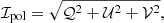
The Stokes parameters, denoted I, Q, U, V, describe the polarization state of a ray by encoding the total intensity of radiation, the intensities of the two types of linear polarization, and the circularly polarized intensity, respectively. The Stokes parameters must be defined in a particular coordinate system such that the wave vector of the associated radiation is parallel to the z-axis of the coordinate system. Their signs are then determined by choosing a convention, that is, a handedness and orientation of the observer coordinate frame. This paper follows the International Astronomical Union (IAU) convention, in which the angle χ = 1/2arctan(U/Q), called the electric vector position angle (EVPA), is defined as an angle east of north, and the sense of circular polarization is called right-handed (left-handed) if the direction of rotation of the EVPA is clockwise (anti-clockwise) for an observer looking in the direction of propagation. For a detailed description of this convention, see, for example, Hamaker & Bregman (1996).
The Stokes parameters are often represented as a vector, the Stokes vector, denoted S = (I, Q, U, V)T. They may also be written in terms of specific intensities, which is convenient for our purpose, as follows: Sν = (Iν, Qν, Uν, Vν)T. The Stokes parameters represent quantities that can be readily measured, hence they are generally used to report observational results.
The Stokes parameters can encode both pure and mixed polarization states; we can distinguish between the two using the degree of polarization, p, which is calculated as follows:
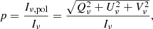 (1)
(1)
where Iν, pol is the intensity of polarized radiation (which is in a pure state, described by Qν, Uν, Vν) and Iν the total intensity. For pure polarization states, this results in p = 1 and Iν, pol = Iν; for mixed states, we have 0 ≤ p < 1 and Iν, pol ≤ Iν. The Stokes parameters omit phase information, and the Stokes vector is not Lorentz covariant. Consequently, to transport the Stokes parameters through curved spacetime consistently, it is necessary to transport a basis vector along the geodesic, even in the case of propagation through a vacuum. Shcherbakov & Huang (2011) present an algorithm that integrates the Stokes parameters directly through curved spacetime in this manner.
Just as the Lorentz-invariant quantity ℐ = Iν/ν3 was employed during integration of the radiative-transfer equation in Bronzwaer et al. (2018), Lorentz-invariant Stokes intensities are defined as follows:
 (2)
(2)
where ν represents the frequency of a ray in the frame in which Sν is evaluated. It is convenient to use these Lorentz-invariant quantities during integration, when constantly shifting between frames.
2.1.2. Polarization four-vector
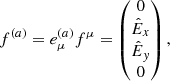
The polarization four-vector, fμ, is a complex-valued vector that describes a pure polarization state. As it is a four-vector, it is Lorentz covariant. The polarization four-vector is a unit vector written as
 (3)
(3)
where the asterisk denotes complex conjugation. The polarization vector associated with a ray is parallel-transported along the null geodesic of the ray as follows:
 (4)
(4)
When expressed in a suitable tetrad frame (see Sect. 2.2) and provided the frame is inertial, meaning that its acceleration vector vanishes, the components of the polarization vector represent normalized, projected electric-field amplitudes along the x and y-axes of the frame, respectively. Using Roman indices framed by parentheses to indicate tetrad-frame coordinates, we have
 (5)
(5)
where  are the components of the ath tetrad-basis vector expressed in coordinates μ, and
  and
and  are components of a unit vector pointing along the electric field. In the most general case, both
  and
and  are complex, and the polarization vector encodes the overall phase of the polarization state. It is also possible to restrict one of the components to be real; only the overall phase information is then lost.
The polarization four-vector only describes pure polarization states; it cannot describe mixed states. However, by keeping track of both the intensity of polarized radiation, ℐpol, and the total intensity ℐ in addition to fμ, it is possible to represent rays with a mixed polarization state.
Given the triplet (ℐ,ℐpol,fμ), plus a suitable tetrad in which to express the Stokes parameters, the transformation (ℐ,ℐpol,f(a)) → 𝒮 is given by
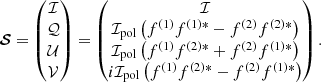 (6)
(6)
The reverse transformation, 𝒮 → (ℐ,ℐpol,f(a)), is degenerate, as the latter quantity contains an additional degree of freedom (the overall phase of the polarization state of the ray). The degeneracy is lifted by choosing a phase, that is, by demanding that f(1) ∈ ℝ. f(a) is then computed as follows:
 (7a)
(7a)
 (7b)
(7b)
 (7c)
(7c)
where  , and similarly for
  and
and  (we note that ℐ retains its identity when transforming).
2.1.3. Spacetime propagation equation
In our model, the polarization state of a ray is affected by two processes: propagation through spacetime and interaction with a plasma. Given Eqs. (1) and (4), we can express the equations of motion for propagation of a polarized ray through curved (vacuum) spacetime as
 (8a)
(8a)
 (8b)
(8b)
 (8c)
(8c)
where λ is the affine parameter expressed in units of length (GM/c2), which parameterizes the null geodesic. The subscript S implies that we only consider effects due to propagation through curved spacetime, ignoring the plasma. Equations (8a)–(8c) show that the degree of polarization p remains constant along a ray when propagated through a curved (vacuum) spacetime. This is a consequence of the fact that Iν, pol and Iν transform in the same way between different frames, so that their ratio remains a constant from frame to frame, and thus throughout a (vacuum) spacetime integration. Equivalently, the corresponding Lorentz-invariant intensities, ℐ and ℐpol, are themselves constant along the ray, as is the ratio between these quantities.
2.2. Constructing suitable tetrad frames to express the Stokes parameters
As in the case of unpolarized radiative transfer, it is convenient to perform the radiative-transfer computations in a suitably chosen frame. Unlike in the case of unpolarized radiative transfer, in which transforming between frames is accomplished simply by computing the frequency of a ray seen by an observer co-moving with the frame of interest, this frame must now be constructed explicitly, as polarized radiative-transfer computations depend on the orientation of the frame. This must be done both at the observer’s location (the camera) and also at any location where the ray interacts with radiating matter. It is also necessary to specify the handedness of the tetrad frame, which is achieved by ordering its basis vectors.
We employed a generalized version of the tetrad described in Gammie & Leung (2012); as is the case for those authors, our tetrad-frame indices (t,∥,⊥,K) correspond with (t,x,y,z), respectively, defining a right-handed coordinate system. As previously, we adopted the (−,+,+,+) metric convention, and we denoted the tetrad-frame coordinates with Roman indices enclosed in parentheses. In what follows, it is assumed that the wave vector of the ray is null (kαkα = 0), that the velocity four-vector of the frame is time-like with norm −1 (i.e., uαuα = −1) and that dα is a space-like vector (dαdα > 0). When the ray resides inside the volume for which GRMHD data is available, uα is given by the local plasma four-velocity, and we may use the local magnetic-field four vector (bα) for the space-like vector dα; bα is space-like (except for the pathological case in which it vanishes, in which case the integration step may be skipped), and orienting the tetrad this way simplifies calculations because all coefficients related to Stokes U vanish. Under these circumstances we refer to the tetrad frame as the plasma frame. When no magnetic-field vector is available, or when we wish to orient the tetrad in a specific way (e.g., to represent a particular observer’s position and attitude), the trial vector dα must be constructed in such a way that it is space-like. This generally happens at the observer’s location, in which case we refer to the tetrad as the observer frame; the velocity four-vector in such cases is generally chosen to be stationary, so that uμ,obs = (ut,0,0,0). Since ut is a constant, the observer frame is an inertial frame. We note that the tetrad must be constructed so as to respect the IAU/IEEE observer convention (Hamaker & Bregman 1996).
To construct a tetrad frame for a ray, we start by defining the intermediate quantities
 (9a)
(9a)
 (9b)
(9b)
 (9c)
(9c)
 (9d)
(9d)
 (9e)
(9e)
The tetrad is then constructed, using the Gram-Schmidt orthonormalization procedure, as follows:
 (10a)
(10a)
 (10b)
(10b)
 (10c)
(10c)
 (10d)
(10d)
where
![Mathematical equation: $$ \begin{aligned} \epsilon ^{\mu \nu \alpha \beta } = -\frac{1}{\sqrt{-g}}\left[ \mu \nu \alpha \beta \right] \ \end{aligned} $$](/articles/aa/full_html/2020/09/aa38573-20/aa38573-20-eq30.gif) (11)
(11)
is the Levi-Civita tensor, [μναβ] is the permutation symbol, and g ≡ det(gμν). We note that the general metric tensor gμν acts on coordinate-frame indices, while the Minkowski metric tensor ημν acts on fluid-frame indices, e.g., gμν → ημν in the fluid frame.
2.3. Plasma interaction: Synchrotron emission, absorption, and Faraday rotation coefficients
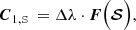
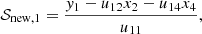
The interaction of the ray with a plasma is most conveniently expressed using the Stokes parameters. Given the plasma frame, we require a set of emission, absorption, and rotation coefficients j, α, and ρ, respectively. The coefficients used in RAPTOR are adapted from Dexter (2016). These are recapitulated in Appendix C. We note that the coefficients must be expressed in their Lorentz-invariant form (Sect. 2.1.1). The effect of the plasma on the invariant Stokes parameters is given by
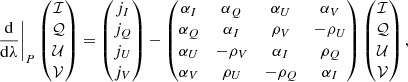 (12)
(12)
where the subscript P implies that only the interaction of the ray with the plasma is taken into account (ignoring the effects due to spacetime propagation).
3. Implementation
In this section, we develop algorithms to implement the polarized radiative-transfer formalism described in Sect. 2 in RAPTOR. The main challenge in this implementation lies in the fact that the polarized radiative-transfer equation (Eq. (12)) may become stiff with respect to explicit integrators depending on the plasma conditions. To mitigate this problem, we analyzed when stiffness occurs and developed an implicit integrator for such integration steps. Precise knowledge of where stiffness occurs is crucial when it comes to minimizing the number of implicit steps, which are less accurate, although much more stable.
3.1. Integration strategy
As in the case of unpolarized radiative transfer through curved spacetime, the integration can be thought of as consisting of two parts: vacuum integration, which takes care of the effects on a polarization state of the ray due purely to traveling through curved spacetime; and plasma integration, which describes the interaction of the ray with the plasma through the emission of the plasma, absorption, and rotation coefficients (Sect. 2.3). The two sub-problems are handled with separate routines. During an integration step and when the ray resides in a radiating plasma, the plasma interaction is computed first, after which a spacetime-propagation step is taken (as if through a vacuum). When the ray resides in vacuum, the plasma-integration step is omitted.
3.2. Numerical scheme for plasma integration
To take the interaction of a ray with the radiating plasma into account, we must solve Eq. (12) numerically. As a consequence of aligning the frame so that the Stokes U polarization mode is parallel to the magnetic-field vector of the plasma, we have jU = αU = ρU = 0. Depending on the local values of the emission, absorption, and rotation coefficients, Eq. (12) may be a stiff equation for explicit integration schemes. The condition for stiffness is different for each explicit integrator and does not directly depend on any particular physical quantity, but rather on the product of the local step size taken by RAPTOR and the largest eigenvalue of the matrix appearing in Eq. (12) (see, e.g., Gautschi 2011). The RAPTOR code uses the fourth-order Runge-Kutta (RK4) explicit integrator (see below); an analysis of when Eq. (12) becomes stiff for the explicit RK4 integrator is presented in Appendix A. The result of that analysis is a numerical stiffness check that is performed at each integration step.
Stiff equations are practically impossible to solve using forward integration methods on the order considered so far in RAPTOR; the solution becomes unstable and prohibitively small step sizes are required. Implicit integration methods are much more stable and can be applied even to stiff problems. However, they tend to dampen rapid oscillations, which increases the stability, but which comes at the cost of less accuracy. In order to integrate Eq. (12), Dexter (2016) employs three integration strategies: an implicit-explicit integrator routine from the LSODA package, an implementation of the DELO method (Rees et al. 1989), and an explicit quadrature method based on the work of Landi Degl’Innocenti & Landi Degl’Innocenti (1985). Mościbrodzka et al. (2016) employed a semi-analytical solution also based on Landi Degl’Innocenti & Landi Degl’Innocenti (1985), along with a three-step numerical integration routine. We choose to develop a novel implicit-explicit integrator for RAPTOR. Since stiffness conditions vary throughout the plasma, using only implicit methods may needlessly sacrifice accuracy in regions where Eq. (12) is not stiff. Switching to an explicit integration scheme in such regions improves the overall accuracy of the computation.
For explicit integration steps, our algorithm uses the following RK4 integrator:
 (13a)
(13a)
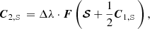 (13b)
(13b)
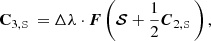 (13c)
(13c)
 (13d)
(13d)
where F represents the right side of Eq. (12). A single explicit integration step proceeds as follows:
 (14)
(14)
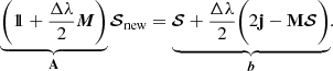
For implicit steps, our algorithm uses the (second-order) implicit trapezoid method given as
![Mathematical equation: $$ \begin{aligned} {\boldsymbol{\mathcal{S} }}_{\rm new} = {\boldsymbol{\mathcal{S} }} + \frac{ \Delta \lambda }{2} \Bigg [ \Big ( \boldsymbol{j} - \boldsymbol{M} {\boldsymbol{\mathcal{S} }}_{\rm new} \Big ) + \Big ( \boldsymbol{j} - \boldsymbol{M} {\boldsymbol{\mathcal{S} }} \Big ) \Bigg ], \end{aligned} $$](/articles/aa/full_html/2020/09/aa38573-20/aa38573-20-eq37.gif) (15)
(15)
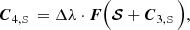
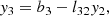
where j = (jI,jQ,jU,jV)T and M is the 4-by-4 matrix appearing in Eq. (12). Since Eq. (12) is linear, the implicit trapezoid method for this equation yields an explicit equation for 𝒮new using an LU-decomposition, so that there is no root-finding penalty even for implicit steps (see Appendix B).
3.3. Numerical scheme for vacuum integration
Previously we integrated the position of the ray, xα, as well as its wave vector, kα, through arbitrary, curved spacetimes. We must now also keep track of the description of the polarization state of the ray, which is captured in the polarization vector fμ; in other words, we must solve Eq. (8a).
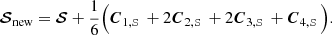
As before, we use a RK4 scheme to integrate the ray backward, that, starting at the camera. After a stopping condition has been reached (e.g., the ray plunges into the horizon or reaches the outer boundary of a GRMHD simulation), polarized radiative transfer proceeds in the forward direction, that is, toward the camera. We extend Eqs. (7)–(14) from Bronzwaer et al. (2018) (noting that forward integration, i.e., from the plasma toward the camera, is employed) to include the polarization vector as follows:
 (16a)
(16a)
 (16b)
(16b)
 (16c)
(16c)
 (16d)
(16d)
where, as in Bronzwaer et al. (2018), underlined indices are a notational shorthand to indicate that all coordinate indices occur on the right-hand side of these equations and Fα represents the right-hand side of Eq. (8a). Given these coefficients, an integration step proceeds as follows:
 (17)
(17)
4. Code verification
In this section we aim to verify the correctness of the output of RAPTOR by comparing it to analytical results and to the output from various codes. For this purpose, a number of verification tests were selected from the literature and reproduced via RAPTOR. Convergence tests were also performed for all integrators described in the previous section.
4.1. Plasma-integration test: Comparison to analytical solution
As a first step, we test our numerical integrator for Eq. (12), that is, the interaction of the ray with the radiating plasma. We note that the two tests reproduced in this section were also reproduced by Dexter (2016) and Moscibrodzka & Gammie (2018), the latter of which performed the test using nonstandard “snake” coordinates, which means that the space-time integration routine is tested simultaneously in their case, making it a more challenging test. In each case, the initial conditions are I = Q = U = V = 0 and the step size is Δs = 0.003.
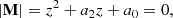
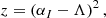
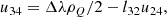
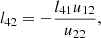
In the first plasma test, jI = 2, jQ = 1, αI = 1, and αQ = 1.2 (all other coefficients vanish). Figure 1 shows the integration results for this test using the RK4 algorithm, while Fig. 2 shows the results for the implicit trapezoid algorithm. In the second plasma test, jQ = jU = jV = 0.1, ρQ = 10, and ρV = −4 (again, all other coefficients vanish). Figure 3 shows the integration results for this test using the RK4 algorithm, while Fig. 4 shows the results for the implicit trapezoid algorithm. We note the difference in the scale of the errors for the implicit trapezoid scheme versus the explicit RK4 scheme – the RK4 scheme, being of a higher order, produces a more accurate result in both cases. On the other hand, the implicit trapezoid scheme is much more robust with respect to increasing the step size, as shown in Fig. 5. Figure 5 repeats the calculation shown in Fig. 4 with a step size that is 100 times larger. Using these settings, the RK4 scheme fails to produce a meaningful result and the error diverges; the trapezoid scheme, on the other hand, remains stable, although the accuracy is affected by the large stepsize.
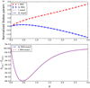 |
Fig. 1. Stokes I and Q (in normalized units) as a function of distance traveled s, using the explicit RK4 integration routine, for the first flat-spacetime plasma-integration test. |
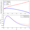 |
Fig. 2. Stokes I and Q (in normalized units) as a function of distance traveled s, using the implicit trapezoid integration routine, for the first flat-spacetime plasma-integration test. |
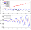 |
Fig. 3. Stokes Q, U, and V (in normalized units) as a function of distance traveled s, using the RK4 integration routine, for the second flat-spacetime plasma-integration test. |
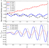 |
Fig. 4. Stokes Q, U, and V (in normalized units) as a function of distance traveled s, using the implicit trapezoid integration routine, for the second flat-spacetime plasma-integration test. |
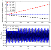 |
Fig. 5. As in Fig. 4, but with a stepsize that is 100 times bigger, so the range of s is 100 times larger as well. |
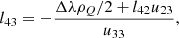
Error-convergence plots for both routines are shown in Figs. 6 and 7; to compute the error for these plots, the absolute difference between the exact and numerical solution was taken at the end of integration, where λ = 3. The fact that the leftmost data point of Fig. 6 is slightly offset from the convergence line suggests that the machine precision, which is of order 1e−16 for the double-precision arithmetic used in RAPTOR, is reached.
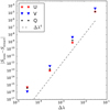 |
Fig. 6. Stepsize-convergence plot for the RK4 plasma-integration routine, for the second plasma test (see Sect. 4.1). The error is proportional to to Δλ4, as expected. |
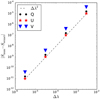 |
Fig. 7. Stepsize-convergence plot for the implicit trapezoid plasma-integration routine for the second plasma test (see Sect. 4.1). The error is proportional to to Δλ2, as expected. |
4.2. Spacetime-integration test: Thin-disk model
Next, we test our integrator for Eq. (8a), that is, the equation for propagation of a polarized ray through spacetime. We do so in a spacetime devoid of matter, save for a geometrically thin, optically thick accretion disk in the equatorial plane, based on the description by Shakura & Sunyaev (1973) and Novikov et al. (1973). The blackbody radiation emitted by the disk is scattered by electrons in the atmosphere of the disk. The radiation is limb-darkened by the atmosphere of the disk and it is partially, linearly polarized in the plane of the disk, perpendicular to both the wave vector and the disk normal, as in the model presented in Chandrasekhar (1960) and studied in Connors et al. (1980) and Schnittman & Krolik (2009). The disk’s atmosphere is not represented in the geometry of the model, but atmospheric effects are taken into account by modifying the emission coefficient. In this model, the emission coefficients are delta functions along the ray; they are evaluated once, after which the polarized light is transported through the vacuum, allowing us to test the vacuum-integration routine; this result was previously reproduced in Dexter (2016).
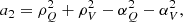
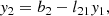
Figure 8 shows the results obtained using the settings specified by an EHT internal note on polarized radiative transfer; these settings are listed in Table 2. The integrated flux densities for all Stokes parameters are reported in Table 1. Although we report the results in units of Jansky per pixel for continuity with the rest of the paper, the camera frequency for this result was in the X-ray part of the electromagnetic spectrum. Figure 9 shows the same result but should be compared with Fig. 1 in Schnittman & Krolik (2009) in the polarization vector representation. Figure 9 also uses a value of 0.9 for the black-hole spin, as did those authors.
 |
Fig. 8. Polarized image of the thin-disk model from Schnittman & Krolik (2009) in terms of the Stokes parameters. The image size is 200 by 200 pixels. Flux is given in Jy px−1 (Jansky per pixel). Stokes V is omitted, as it vanishes owing to the symmetry of the problem. |
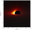 |
Fig. 9. Polarized image of the thin-disk model from Schnittman & Krolik (2009) shown with polarization vectors. |
Figure 10 shows the stepsize-convergence plot for the RK4 spacetime-integration routine (which integrates Eq. (8a)). The error was computed by tracking the norm of the polarization vector, which should be conserved after integration of the ray; the ray passes close to the black hole through a strongly curved region of spacetime.
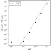 |
Fig. 10. Stepsize-convergence plot for the RK4 spacetime-transport routine, for a particular ray in the thin-disk test (see Sect. 4.2). The error is proportional to to Δλ4, as expected. |
4.3. Spacetime-and-plasma (GRMHD) integration test
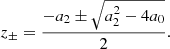
Finally, we tested the combination of the vacuum and plasma-integration routines. To do so, the rays must propagate through a radiating plasma that is of finite extent (i.e., not infinitesimally thin), so that plasma interaction takes place as the rays are propagating through curved spacetime. This may be achieved using data from a GRMHD simulation of an accreting AGN; a particular data dump, created using the HARM code (Gammie et al. 2003), was used for these tests, which are part of the EHT internal code comparison for polarized radiative transfer, a forthcoming publication. The radiative model uses the thermal-synchrotron emission, absorption, and rotation coefficients listed in Appendix C, and a constant proton-to-electron temperature ratio of 3, making this a disk-dominated emission model. To reproduce the results listed in this paper, please refer to Table 2, which shows the RAPTOR settings used to generate the test results for two scenarios (the low-accretion-rate and high-accretion-rate scenarios, respectively); the GRMHD dump that was used to generate these results is distributed along with RAPTOR. The resulting images (Figs. 11 and 12) show a low-luminosity AGN at a low inclination angle (163 degrees or 17 degrees from the southern pole). A radial pattern is observed. Table 1 lists the flux densities obtained for the thin-disk and GRMHD tests.
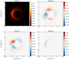 |
Fig. 11. Polarized image of the GRMHD-based third test for the high-accretion-rate scenario. A different field of view from the original test (see Table 2) enhances the clarity of the images; the camera size for these images is 20 by 20 RG, and the image size is 1024 by 1024 pixels. Flux is given in Jy px−1 (Jansky per pixel). The integrated flux densities, useful for code-comparison purposes, are recapitulated in Table 1. |
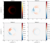 |
Fig. 12. Polarized image of the GRMHD-based third test for the low-accretion-rate scenario. A different field of view from the original test (see Table 2) enhances the clarity of the images; the camera size for these images is 20 by 20 RG, and the image size is 1024 by 1024 pixels. Flux is given in Jy px−1 (Jansky per pixel). The integrated flux densities, useful for code-comparison purposes, are recapitulated in Table 1. |
4.4. Convergence with other polarized radiative-transfer codes
The thin-disk and GRMHD tests discussed in the previous two sections were adopted by the collaborative effort by the EHT to establish convergence between polarized GRRT codes, which is to be published in a forthcoming paper. At the time of publication, comparison to ipole output for the same tests yielded an agreement to order 1% in terms of mean squared error. Experience has revealed a few possible sources of error, such as the precise camera setup used, or the approximations used to compute Bessel functions in the emission/absorption/rotation coefficients. However, since there are uncertainties that are larger than 1% in such aspects of the computation as the microphysics (e.g., the energy-distribution functions of the radiating electrons, which is affected by magnetic reconnection, fine-scale turbulence, and shockwaves), the agreement that has been achieved is sufficient for current EHT science goals. Nevertheless, these results may be refined further and are to be published in a forthcoming EHT paper comparing methods for polarized GRRT.
5. Summary
We have developed a code capable of performing efficient polarized radiative transfer in arbitrary spacetimes to deepen the understanding of polarized observations of astrophysical phenomena originating in strong gravitational fields. Our implementation can represent a polarized ray using both the Stokes vector and the polarization vector (plus relevant intensities) and can switch between the two. The former description is appropriate for plasma interactions, whenever the ray is inside a plasma, while the latter presents a better description for spacetime propagation. This formalism is conceptually simple and uses the minimum number of degrees of freedom.
The polarized radiative-transfer equation, which describes the interaction of a ray with a plasma, may become stiff in some regions of the integration volume, while being much easier to integrate in others. We developed a computationally efficient, yet robust, implicit-explicit scheme to integrate this equation. Our algorithm switches between implicit and explicit integration schemes to maximize accuracy and efficiency. We determined when the polarized radiative-transfer equation (as expressed in our particular tetrad frame) becomes stiff for the RK4 integrator to establish the switching criterium.
We demonstrated the correctness of our new algorithms for spacetime propagation and plasma interaction separately as well as together. A comparison of RAPTOR output for the thin-disk and GRMHD tests described in Sects. 4.2 and 4.3 to that of ipole show excellent agreement; this strongly suggests that the two different implementations agree on the physics to a sufficient degree of accuracy for the EHT in the context of a relevant, complex astrophysical problem. The value in that result lies both in adding credence to the theoretical calculations of the EHT pertaining to polarized sources such as M87, and in providing a new, public tool for the efficient production of simulated, polarized observations.
Polarized observations have the potential to allow observers to determine the structure of magnetic fields in the accretion disks and jets of black holes. Meanwhile, theoretical investigations probe the observational effects produced by various plasma models (see, e.g., Jiménez-Rosales & Dexter 2018; Palumbo et al. 2020) and even different theories of gravity (Mizuno et al. 2018). The RAPTOR code can be used as an efficient and flexible tool with which to explore the radiative properties of various plasma models in arbitrary spacetimes. Such simulations can be compared with current and future observations of polarized radiation emitted by the orbiting black holes, neutron stars, and potentially other, more exotic objects.
Acknowledgments
This work is supported by the ERC Synergy Grant “BlackHoleCam: Imaging the Event Horizon of Black Holes” (Grant 610058). ZY is supported by a Leverhulme Trust Early Career Fellowship. The authors thank Koen de Boer, Monika Mościbrodzka, Ben Prather, George Wong, and the anonymous referee for their helpful suggestions regarding the manuscript. This work has made use of NASA’s Astrophysics Data System (ADS).
References
- Aitken, D. K., Greaves, J., Chrysostomou, A., et al. 2000, ApJ, 534, L173 [Google Scholar]
- Bower, G. C., Wright, M. C. H., Falcke, H., & Backer, D. C. 2003, ApJ, 588, 331 [Google Scholar]
- Broderick, A. E. 2006, MNRAS, 366, L10 [Google Scholar]
- Broderick, A., & Blandford, R. 2004, MNRAS, 349, 994 [Google Scholar]
- Broderick, A. E., & Loeb, A. 2006, MNRAS, 367, 905 [Google Scholar]
- Broderick, A. E., & Narayan, R. 2006, ApJ, 638, L21 [Google Scholar]
- Bromley, B. C., Melia, F., & Liu, S. 2001, ApJ, 555, L83 [Google Scholar]
- Bronzwaer, T., Davelaar, J., Younsi, Z., et al. 2018, A&A, 613, A2 [NASA ADS] [CrossRef] [EDP Sciences] [Google Scholar]
- Chandrasekhar, S. 1960, Radiative Transfer (New York: Dover) [Google Scholar]
- Connors, P. A., Piran, T., & Stark, R. F. 1980, ApJ, 235, 224 [Google Scholar]
- Davis, L. J., & Greenstein, J. L. 1951, ApJ, 114, 206 [Google Scholar]
- Dexter, J. 2016, MNRAS, 462, 115 [NASA ADS] [CrossRef] [Google Scholar]
- Dexter, J., & Agol, E. 2009, ApJ, 696, 1616 [Google Scholar]
- Dexter, J., Agol, E., & Fragile, P. C. 2009, ApJ, 703, L142 [Google Scholar]
- Event Horizon Telescope Collaboration 2019, ApJ, 875, L1 [Google Scholar]
- Falcke, H., & Biermann, P. L. 1995, A&A, 293, 665 [NASA ADS] [Google Scholar]
- Falcke, H., Melia, F., & Agol, E. 2000, ApJ, 528, L13 [Google Scholar]
- Falcke, H., Nagar, N. M., Wilson, A. S., Ho, L. C., & Ulvestad, J. S. 2001, in Radio Cores in Low-Luminosity AGN: ADAFs or Jets?, eds. L. Kaper, E. P. J. V. D. Heuvel, & P. A. Woudt, Black Holes in Binaries and Galactic Nuclei, 218 [Google Scholar]
- Falcke, H., Körding, E., & Markoff, S. 2004, A&A, 414, 895 [NASA ADS] [CrossRef] [EDP Sciences] [Google Scholar]
- Gabuzda, D. C., & Cawthorne, T. V. 2000, MNRAS, 319, 1056 [Google Scholar]
- Gabuzda, D. C., Sitko, M. L., & Smith, P. S. 1996, AJ, 112, 1877 [Google Scholar]
- Gammie, C. F., & Leung, P. K. 2012, ApJ, 752, 123 [Google Scholar]
- Gammie, C. F., McKinney, J. C., & Tóth, G. 2003, ApJ, 589, 444 [Google Scholar]
- Gautschi, W. 2011, Numerical Analysis (Basel: Birkhäuser) [Google Scholar]
- Goddi, C., Falcke, H., Kramer, M., et al. 2017, Int. J. Mod. Phys. D, 26, 1730001 [Google Scholar]
- Gralla, S. E., Holz, D. E., & Wald, R. M. 2019, Phys. Rev. D, 100, 024018 [Google Scholar]
- Gravity Collaboration (Abuter, R., et al.) 2018, A&A, 618, L10 [NASA ADS] [CrossRef] [EDP Sciences] [Google Scholar]
- Hada, K., Kino, M., Doi, A., et al. 2016, ApJ, 817, 131 [Google Scholar]
- Hamaker, J. P., & Bregman, J. D. 1996, A&AS, 117, 161 [NASA ADS] [CrossRef] [EDP Sciences] [Google Scholar]
- Heeschen, D. S. 1970, AJ, 75, 523 [Google Scholar]
- Jaroszynski, M., & Kurpiewski, A. 1997, A&A, 326, 419 [Google Scholar]
- Jiménez-Rosales, A., & Dexter, J. 2018, MNRAS, 478, 1875 [Google Scholar]
- Johnson, M. D., Fish, V. L., Doeleman, S. S., et al. 2015, Science, 350, 1242 [Google Scholar]
- Jones, T. W., & Hardee, P. E. 1979, ApJ, 228, 268 [Google Scholar]
- Landi Degl’Innocenti, E., & Landi Degl’Innocenti, M. 1985, Sol. Phys., 97, 239 [NASA ADS] [CrossRef] [Google Scholar]
- Lyutikov, M., Pariev, V. I., & Gabuzda, D. C. 2005, MNRAS, 360, 869 [NASA ADS] [CrossRef] [Google Scholar]
- Misner, C. W., Thorne, K. S., & Wheeler, J. A. 1973, Gravitation (San Francisco: W. H. Freeman and Co.) [Google Scholar]
- Mizuno, Y., Younsi, Z., Fromm, C. M., et al. 2018, Nat. Astron., 2, 585 [Google Scholar]
- Moscibrodzka, M., & Gammie, C. F. 2018, MNRAS, 475, 43 [Google Scholar]
- Moscibrodzka, M., Gammie, C., Dolence, J., Shiokawa, H., & Leung, P. 2009, in Radiative Models of Sgr A* from GRMHD Simulations, eds. S. Wolk, A. Fruscione, & D. Swartz, Chandra’s First Decade of Discovery [Google Scholar]
- Mościbrodzka, M., Falcke, H., & Shiokawa, H. 2016, A&A, 586, A38 [NASA ADS] [CrossRef] [EDP Sciences] [Google Scholar]
- Narayan, R., Mahadevan, R., & Quataert, E. 1998, in Advection-dominated Accretion Around Black Holes, eds. M. A. Abramowicz, G. Björnsson, & J. E. Pringle, Theory of Black Hole Accretion Disks, 148 [Google Scholar]
- Narayan, R., Johnson, M. D., & Gammie, C. F. 2019, ApJ, 885, L33 [Google Scholar]
- Noble, S. C., Leung, P. K., Gammie, C. F., & Book, L. G. 2007, CQG, 24, 259 [Google Scholar]
- Novikov, I. D., & Thorne, K. S. 1973, in Black Holes (Les Astres Occlus), eds. C. Dewitt, & B. S. Dewitt, Astrophys. Black Holes, 343 [Google Scholar]
- Palumbo, D. C. M., Wong, G. N., & Prather, B. S. 2020, ApJ, 894, 156 [Google Scholar]
- Rees, D. E., Murphy, G. A., & Durrant, C. J. 1989, ApJ, 339, 1093 [Google Scholar]
- Schnittman, J. D., & Krolik, J. H. 2009, ApJ, 701, 1175 [CrossRef] [Google Scholar]
- Shakura, N. I., & Sunyaev, R. A. 1973, A&A, 500, 33 [NASA ADS] [Google Scholar]
- Shcherbakov, R. V., & Huang, L. 2011, MNRAS, 410, 1052 [Google Scholar]
- Wrobel, J. M., & Heeschen, D. S. 1991, AJ, 101, 148 [Google Scholar]
- Younsi, Z., Porth, O., Mizuno, Y., Fromm, C. M., & Olivares, H. 2020, in Modelling the Polarised Emission from Black Holes on Event Horizon-Scales, eds. K. Asada, E. de Gouveia Dal Pino, M. Giroletti, H. Nagai, & R. Nemmen, IAU Symp., 342, 9 [Google Scholar]
- Younsi, Z., Wu, K., & Fuerst, S. V. 2012, A&A, 545, A13 [NASA ADS] [CrossRef] [EDP Sciences] [Google Scholar]
- Yuan, F., Quataert, E., & Narayan, R. 2003, ApJ, 598, 301 [NASA ADS] [CrossRef] [Google Scholar]
Appendix A: Stiffness analysis of the polarized radiative-transfer equation
The stiffness of a linear system of differential equations, such as the polarized radiative-transfer equation (Eq. (12)), with respect to a particular explicit integration scheme (such as the RK4 integrator used here), depends on the eigenvalues of the matrix that appears on the right-hand side of that equation, M; our first step is to compute these eigenvalues.
In a frame in which jU = αU = ρU = 0, M’s characteristic polynomial is given by
 (A.1)
(A.1)
where
 (A.2a)
 (A.2b)
 (A.2c)
where Λ us an eigenvalue of M. In other words, M’s characteristic polynomial is a biquadratic equation in (αI−Λ), which may therefore be obtained by solving the quadratic equation
 (A.3)
(A.3)
There are then four possible values for (αI−Λ), that is,
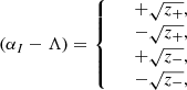 (A.4a)
so that
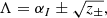 (A.5)
(A.5)
where either plus/minus symbol may be interpreted in either way.
Now that M’s eigenvalues are known, the stiffness of Eq. (12) for the explicit RK4 integrator can be computed. Defining
 (A.6)
(A.6)
where Δλ is integration step size of RAPTOR, the explicit RK4 integration routine is stable when
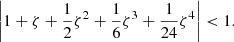 (A.7)
(A.7)
Whenever this condition is not met for any one of M’s four eigenvalues, it is necessary to switch to the implicit trapezoid integration routine.
Appendix B: Implicit trapezoid integrator
Rewriting Eq. (15), we obtain a system of equations for 𝒮new as follows:
 (B.1)
(B.1)
The matrix A, evaluated in a frame in which jU, αU, and ρU vanish, is then given by
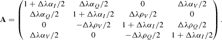 (B.2)
(B.2)
Next, we express A as a product of two triangular matrixes, L and U:
 (B.3)
(B.3)
whose elements are given by
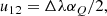
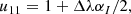 (B.4a)
 (B.4b)
 (B.4c)
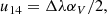 (B.4d)
 (B.4e)
 (B.4f)
 (B.4g)
 (B.4h)
 (B.4i)
 (B.4j)
 (B.4k)
 (B.4l)
 (B.4m)
 (B.4n)
 (B.4o)
 (B.4p)
This allows us to obtain 𝒮new explicitly, from two linear systems of equations, that is,
 (B.5a)
 (B.5b)
where y’s components are given by
 (B.6a)
 (B.6b)
 (B.6c)
 (B.6d)
𝒮new is then computed as follows:
 (B.7a)
 (B.7b)
 (B.7c)
 (B.7d)
Appendix C: Emission, absorption, and rotation coefficients for a thermal electron population
This appendix lists the emission, absorption, and rotation coefficients employed in RAPTOR. These coefficients pertain to a (relativistic) thermal distribution of electrons. They are adapted from Dexter (2016) (nonthermal (power-law) coefficients are also listed in that paper), with a number of modifications of numerical fit functions by Moscibrodzka & Gammie (2018), as well as minor notational rewrites in Eqs. (C.6b) and typographical corrections in Eq. (C.10) (cf. B14 in Dexter 2016).
The emission coefficients are given by
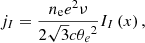 (C.1a)
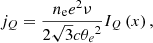 (C.1b)
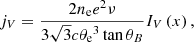 (C.1c)
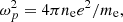
where ne is the electron number density, e is the electron charge, c is the speed of light, θe is the dimensionless electron temperature, θB is the angle between the wave vector and the magnetic-field vector, and x is the ratio of the frequency of the ray over the critical plasma frequency as follows:
 (C.2)
(C.2)
where
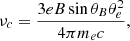 (C.3)
(C.3)
with B being the magnetic-field amplitude (in Gaussian-cgs units).
The expressions II, IQ, IV represent numerical fit functions, and are given by
 (C.4a)
 (C.4b)
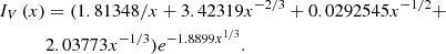 (C.4c)
Absorption is computed using Kirchoff’s law, as the distribution is thermal, so that the absorption coefficients may be written as
 (C.5)
(C.5)
where Bν is the blackbody function.
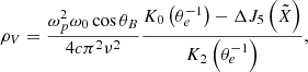
Finally, the rotation coefficients are given by
![Mathematical equation: $$ \begin{aligned}&\rho _Q = \frac{ \omega _p^2 \omega _0^2 \sin ^2{\theta _B}}{16 c \pi ^3 \nu ^3 } f_m\left( \tilde{X} \right) + \left[ \frac{K_1\left( \theta _e^{-1} \right)}{K_2\left(\theta _e^{-1} \right)} + 6 \theta _e \right], \end{aligned} $$](/articles/aa/full_html/2020/09/aa38573-20/aa38573-20-eq90.gif) (C.6a)
(C.6a)
 (C.6b)
where
 (C.7)
(C.7)
 (C.8)
(C.8)
and
 (C.9)
(C.9)
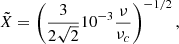
The functions fm and ΔJ5 again represent fit functions. They are given by
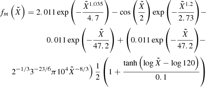 (C.10)
and
 (C.11)
respectively.
We note that during a RAPTOR run, the Lorentz-invariant versions of these coefficients are employed. Transforming the emission, absorption, and rotation coefficients to their Lorentz-invariant forms proceeds as follows:
 (C.12a)
 (C.12b)
 (C.12c)
All Tables
All Figures
|
Fig. 1. Stokes I and Q (in normalized units) as a function of distance traveled s, using the explicit RK4 integration routine, for the first flat-spacetime plasma-integration test. |
| In the text | |
|
Fig. 2. Stokes I and Q (in normalized units) as a function of distance traveled s, using the implicit trapezoid integration routine, for the first flat-spacetime plasma-integration test. |
| In the text | |
|
Fig. 3. Stokes Q, U, and V (in normalized units) as a function of distance traveled s, using the RK4 integration routine, for the second flat-spacetime plasma-integration test. |
| In the text | |
|
Fig. 4. Stokes Q, U, and V (in normalized units) as a function of distance traveled s, using the implicit trapezoid integration routine, for the second flat-spacetime plasma-integration test. |
| In the text | |
|
Fig. 5. As in Fig. 4, but with a stepsize that is 100 times bigger, so the range of s is 100 times larger as well. |
| In the text | |
|
Fig. 6. Stepsize-convergence plot for the RK4 plasma-integration routine, for the second plasma test (see Sect. 4.1). The error is proportional to to Δλ4, as expected. |
| In the text | |
|
Fig. 7. Stepsize-convergence plot for the implicit trapezoid plasma-integration routine for the second plasma test (see Sect. 4.1). The error is proportional to to Δλ2, as expected. |
| In the text | |
|
Fig. 8. Polarized image of the thin-disk model from Schnittman & Krolik (2009) in terms of the Stokes parameters. The image size is 200 by 200 pixels. Flux is given in Jy px−1 (Jansky per pixel). Stokes V is omitted, as it vanishes owing to the symmetry of the problem. |
| In the text | |
|
Fig. 9. Polarized image of the thin-disk model from Schnittman & Krolik (2009) shown with polarization vectors. |
| In the text | |
|
Fig. 10. Stepsize-convergence plot for the RK4 spacetime-transport routine, for a particular ray in the thin-disk test (see Sect. 4.2). The error is proportional to to Δλ4, as expected. |
| In the text | |
|
Fig. 11. Polarized image of the GRMHD-based third test for the high-accretion-rate scenario. A different field of view from the original test (see Table 2) enhances the clarity of the images; the camera size for these images is 20 by 20 RG, and the image size is 1024 by 1024 pixels. Flux is given in Jy px−1 (Jansky per pixel). The integrated flux densities, useful for code-comparison purposes, are recapitulated in Table 1. |
| In the text | |
|
Fig. 12. Polarized image of the GRMHD-based third test for the low-accretion-rate scenario. A different field of view from the original test (see Table 2) enhances the clarity of the images; the camera size for these images is 20 by 20 RG, and the image size is 1024 by 1024 pixels. Flux is given in Jy px−1 (Jansky per pixel). The integrated flux densities, useful for code-comparison purposes, are recapitulated in Table 1. |
| In the text | |
Current usage metrics show cumulative count of Article Views (full-text article views including HTML views, PDF and ePub downloads, according to the available data) and Abstracts Views on Vision4Press platform.
Data correspond to usage on the plateform after 2015. The current usage metrics is available 48-96 hours after online publication and is updated daily on week days.
Initial download of the metrics may take a while.