| Issue |
A&A
Volume 641, September 2020
|
|
|---|---|---|
| Article Number | A108 | |
| Number of page(s) | 7 | |
| Section | Planets and planetary systems | |
| DOI | https://doi.org/10.1051/0004-6361/202038556 | |
| Published online | 16 September 2020 | |
The orbit of Triton with new precise observations and the INPOP19a ephemeris
1
Shanghai Astronomical Observatory, Chinese Academy of Sciences,
80 Nandan Road,
Shanghai
200030,
PR China
e-mail: This email address is being protected from spambots. You need JavaScript enabled to view it.
2
National Time Service Center, Chinese Academy of Sciences,
No.3 East Shuyuan Road,
Lintong,
Shaanxi
710600,
PR China
3
School of Astronomy and Space Science, University of Chinese Academy of Sciences,
No.19(A) Yuquan Road,
Shijingshan District,
Beijing
100049, PR China
4
School of Fundamental Studies, Shanghai University of Engineering Science,
333 Long Teng Road,
Shanghai
201620,
PR China
5
School of Physics and Electronic Information, Huanggang Normal University,
146 Xingang Second Road,
Huanggang,
Hubei
438000, PR China
Received:
2
June
2020
Accepted:
30
June
2020
Abstract
Aims. The Gaia catalogue brings new opportunities and challenges to high-precision astronomy and astrometry. The precision of data reduction is therefore improved by a large number of reference stars with high-precision positions and proper motions. Numerous precise positions for Triton are obtained from the latest observations using the Gaia catalogue. Furthermore, the new INPOP19a planetary ephemeris, which also fits the observations from the Gaia Data Release 2, has recently become available. In this paper, a new orbit of Triton is calculated using the latest precise charge-coupled device (CCD) observations and the INPOP19a ephemeris.
Methods. Triton’s orbital solution is calculated using a numerical integrator, while the orientation of Neptune’s pole in particular is obtained by integrating the simplified Euler’s equations of motion. We determine the orbit of Triton over 170 yr based on 11 040 Earth-based observations made between 1847 and 2016 and on Voyager 2 data. The positions of the Sun and planets are provided by the INPOP19a ephemeris. We compare our results to those from other previous works to check the influences on Triton’s orbit from different planetary ephemerides.
Results. A new orbit of Triton is provided here. The root-mean-square of the residuals for the Earth-based CCD absolute observations are 0.102″ in right ascension and 0.142″ in declination. Although most different planetary ephemerides have large differences in Neptune’s position, the orbits of Triton using different planetary ephemerides are still close, under similar dynamical models. The Voyager 2 data add a constraint on Triton’s orbit here.
Key words: astrometry / celestial mechanics / ephemerides / planets and satellites: individual: Neptune / planets and satellites: individual: Triton
© ESO 2020
1 Introduction
Triton is the largest satellite in the Neptunian system. Due to its inclined retrograde orbit, Triton is very likely a captured Kuiper belt object and holds the answers to questions about the icy dwarf planets that formed in the outer Solar System (Masters et al. 2014). Since its discovery in 1846, Triton has continually been observed via visual, photographic, and charge-coupled device (CCD) techniques. The close detection of the Neptunian system was only achieved by the Voyager 2 spacecraft on August 25, 1989. Voyager 2 has provided the most accurate data for Triton to date. All these observations provide an opportunity to determine Triton’s orbit and improve the related dynamical model.
After the Voyager 2 Neptune detection, the precise numerical model of Triton’s motion and the orientation of Neptune’s pole was provided by Jacobson (2009). All parameters in this Neptunian dynamical model were fitted by the Earth-based observations made between 1847 and 2008 and by the Voyager 2 data. This ephemeris of Triton also displays good consistency with the latest observations. Another orbital determination of Triton was presented by Zhang et al. (2014). It was based on Earth-based observations made during the period 1975–2006 and differs slightly from Jacobson (2009)’s results, within 0.1″ in Triton’s absolute position over 32 yr. In addition, Poroshina (2013) attempted to use the Russian planetary ephemeris EPM2008 and the Jet Propulsion Laboratory planetary ephemeris DE405 to obtain a numerical ephemeris of Triton. Compared with the above numerical ephemerides, the analytical theory of Triton’s motion given by Emelyanov & Samorodov (2015) has the advantage of easy programming. It enables us to calculate the ephemeris for any instant of time by using simple formulas, with sufficient precision.
The errors in the dynamical model could seriously affect the orbit accuracy. In Triton’s case, the uncertainty in Neptune’s pole orientation and Neptune’s gravitational harmonics are the primary considerations (Jacobson 2009). In Jacobson (2009), Neptune’s polar motion is only driven by the torque due to the gravitational attraction of Triton on the planet’s equatorial bulge. The total angular momentum of the system, which includes the angular momentum of Neptune and the angular momentum of Triton’s mean orbit, is presumed to be constant. Neptune’s pole model is provided as a unit vector that precesses at a constant rate about an axis aligned with the Neptunian system angular momentum vector. The pole’s orientation angles are expressed by the angles related to Triton’s orbit and the system angular momentum. In this paper, we calculate the pole’s motion by integrating simplified Euler’s equations of motion. This could help with further investigations into the Neptunian system.
Furthermore, the new Gaia catalogue offers new opportunities and challenges for high-precision astrometry. A large number of reference stars with high-precision positions and proper motions are provided. This improves the precision of data reduction. Even early CCD images can be re-processed and provide very accurate position results (Yan et al. 2020). All these new precious observationscould contribute to ephemeris precision. Here, a new ephemeris of Triton is obtained, which notably fits the latest precise positions of Triton.
For most different planetary ephemerides, the positions of Neptune and Uranus have larger differences. This may affect the integration of Triton’s motion and Triton’s observation residuals. The new IMCCE planetary ephemeris INPOP19a has recently become available (Fienga et al. 2019). We used INPOP19a for all of our calculations; we compare our results with those from Jacobson (2009), who used DE421 to check the planetary ephemerides’ influences on Triton’s orbit.
In this paper, a new orbit of Triton is presented. In Sect. 2, we describe our numerical model for Triton’s orbit. Section 3 outlines the observations we use. The orbit of Triton is given in Sect. 4. Finally, the influences on Triton’s orbit due to different planetary ephemerides are discussed in Sect. 5.
2 Numerical model
Triton’s motion is modelled on the Neptunian barycentric reference system, with its origin at the Neptunian system barycenter, and its orientation is determined by the international celestial reference frame (ICRF). Barycentric dynamical time (TDB) is used as the coordinate time. Triton’s orbit is dominated by Neptune’s gravitation and perturbed by the Sun and other planets of the Solar System. Other Neptune satellites are rather small and their influences can be neglected. The figure effect from the second and fourth zonal harmonics of Neptune’s gravity field is also taken into account. However, other effects are too small to be considered here.
The Neptune figure effect depends on the motion of its pole, which includes precession and nutation. Since we lack sufficient direct information for the planet, Neptune is assumed to be an axially symmetric rigid body as an expedient for calculating its rotational motion, as in Jacobson (1990). Furthermore, we only considered Triton’s torque acting on Neptune’s equatorial bulge. Neptune’s orientation can be given by two Euler angles, φ and θ, which relate an intermediate reference system O − X′Y′Z′ from the Neptunian reference system by applying the rotation R1(θ)R3(φ). The Z′ axis of this intermediate reference system is aligned with Neptune’s pole. Based on the assumption above, the second derivatives of the Euler angles could be obtained by using Euler’s equations and neglecting the high order items:

where ω is Neptune’s spin rate; A and C are the equatorial and polar moment of inertia and are related to Neptune’s axial moment of inertia factor γ, the equatorial radius R, and Neptune’s quadrupole moment J2 (Jacobson 1990); and T is the torque. The relations between the Euler angles and right ascension αN and declination δN of the pole are:
 (3)
(3)
 (4)
(4)
Therefore, Triton’s orbital solution is calculated using a numerical integrator, while the orientation of Neptune’s pole is obtained by integrating the simplified Euler’s equations of motion. All the motions were calculated in the Neptunian reference system using a Bulirsch-Stoer integrator, which is suitable for most kinds of orbit (Huang 1990). The step size is set to 0.1 days. The Bulirsch-Stoer algorithm exploits the midpoint method, which computes the values of the dependent variables via a sequence of substeps to get good accuracy in each step. Compensated summation is used to reduce round-off errors. The positions of the Sun and planets are from INPOP19a. The initial condition of the Euler angles and their derivatives at t0 = 2 447 763.5 (TDB), the date of Voyager 2’s close detection of Neptune, are derived from Jacobson (2009):
 ,
,
 ,
,
 ,
,
 .
.
Other parameters used here are given in Table 1.
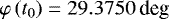
The motion of Neptune’s pole is calculated over the period 1847–2016. Figure 1 shows the differences regarding right ascension and declination of Neptune’s pole between our result and the pole’s model in Jacobson (2009). The pole’s nutation is reflected in the thickness of the curves. The discrepancies are smaller than 2.5″. This demonstrates that the calculations of Neptune’s polar motion are close, by the integration of the pole’s motion or through the constant total angular momentum.
Dynamical parameters (values are from Jacobson 2009).
3 Observations
Triton has been continuously observed since 1846 and a large accumulation of relative and absolute observations, including visual, photographic, and CCD data, are available. Most of these data are available on the Natural Satellite Ephemeride Server MULTI-SAT website (Emel’Yanov & Arlot 2008). To determine Triton’s orbit, we used Earth-based observations made between 1847 and 2016 in addition to Voyager 2 observations.
All the observations we used are listed in Tables A.1 and A.2. The historical observations are sorted as they are in Emelyanov & Samorodov (2015). The observation year, observatory code, source, and type of these observationsare listed in these tables. The types are described as: “P,S” position angle and angular separation; “α,δ” right ascension and declination; and “X,Y ” X = dαcosδ and Y = dδ, where d α and d δ are the differences in right ascension and declination between the satellite and reference body. The observations were selected using the three-sigma rule for outlier detection, and 309 of them were rejected. There were six main differences between the observations used in this paper and those used by Emelyanov & Samorodov (2015), which consist of: (1) the observations from the Greenwich Royal Observatory (1899–1907; Christie 1901, 1904, 1909); (2) the Voyager 2 data (Jacobson 1991), which were processed in the FK4/B1950 system and still provide position results with sufficiently high precision; (3) the observations from the Sheshan Station of the Shanghai Astronomical Observatory (1996–2006; Qiao et al. 2007), which were re-reduced by Yan et al. (2020) using the Gaia Data Release (DR) 2 and solved the systematic errors from the inaccuracy of the UCAC2 catalogue; (4) the observations from the Table Mountain Observatory (2001–2012)1; (5) the observations from the United States Naval Observatory Flagstaff Station (2013–2014)2; (6) the precise data from the Yunnan Observatory (2014–2016; Wang et al. 2017), which were reduced using the Gaia DR1.
In total, 11 040 Earth-based observations from 1847 to 2016 and the Voyager 2 data are used. Compared with Jacobson (2009), We use an additional 1 306 observations that were collected during the period 2009–2016. All these data are used for determining the epoch state vectors of Triton. In the future, more precise observations using the Gaia catalogue will be available and contribute to the ephemeris precision.
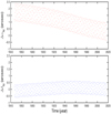 |
Fig. 1 Differences in right ascension (top panel) and declination (bottom panel) of Neptune’s pole between our results and Jacobson (2009)’s results during the period 1847–2016. |
4 Triton’s orbit
Here only the epoch state vectors of Triton are fitted to observations. Other parameters in our dynamical model are fixed, as mentioned in Sect. 2. The initial date of Triton’s orbit integration is set to t0 = 2 447 763.5 (TDB), the same as that of the Euler angles. The initial condition of Triton’s orbit is taken from Jacobson et al. (1991). The planetary ephemeris used here is INPOP19a. The principle for orbit determination is from Tapley et al. (2004). The data weights are determined by the associated error covariance matrix, and a priori information about the accuracy of the initial state vectors is estimated.
After the fitting process, Table 2 gives the final state vectors of Triton at t0 , given with respect to the Neptunian barycentric reference system. The observation residuals with this orbit are given in Tables A.1 and A.2. The last three columns of these two tables are the number of the observations we use and the root-mean-square (RMS) of the residuals for the different types of observations. Figure 2 shows the observed minus calculated (O–C) residuals in different types for all the observations. The scale of the vertical axis for type P is distinguished from the others. The RMS of the residuals for the Earth-based CCD absolute observations is 0.102″ in right ascension and 0.142″ in declination.
To estimate the accuracy of our Triton orbit, we compared our results with the results from Jacobson (2009) and the DE431 ephemeris, which are from the MULTI-SAT website (Emel’Yanov & Arlot 2008). The differences in X(d αcosδ) and Y (d δ) between our results and the Jacobson (2009) results are shown in Fig. 3. The differences in relative position are less than 0.02″. This indicates that these two Triton orbits are very close from 1847 to 2016. We also compared our results with the Jacobson (2009) results regarding Triton’s absolute position. The differences are depicted in Fig. 4 and are around 0.8″ in right ascension and 0.3″ in declination near 1847. All these discrepancies mostly come from differences in Neptune’s position relative to the Earth between INPOP19a and DE431. It shows that the absolute position of Triton is dependent on the planetary ephemeris used, while the relative position is much less so.
Neptunian barycentric state vectors of Triton at Julian day (TDB) 2 447 763.5 (Aug. 25, 1989).
5 The influences of different planetary ephemerides on Triton’s orbit
Our calculations were carried out with the INPOP19a ephemeris, while Jacobson (2009) used DE421. Although most different planetary ephemerides have large differences in Neptune’s position, the orbits of Triton using different planetary ephemeridesare still close, under the similar dynamical model (see Sect. 4). We also used INPOP17a (Viswanathan et al. 2017) and DE430 (Folkner et al. 2014) to re-determine Triton’s orbit. Similar results confirm this conclusion.
To determine the reason why the orbits of Triton found using different planetary ephemerides are close, we refitted the orbits to different observation sets. The Voyager 2 data are found to be the key point for this. Without Voyager 2 observations, the re-determined orbits of Triton with different planetary ephemerides have larger discrepancies. The Voyager 2 data add a strong constraint on the positions of Neptune and Triton. They provide position measures with an accuracy ranging from a few hundred kilometres to better than 5 km , depending on the distance between the spacecraft and satellite (Jacobson 2009). Furthermore, most different planetary ephemeridesprovide a similar position for Neptune near the Voyager 2 Neptune encounter; the differences then increase with time.
Poroshina (2013) only used Earth-based observations made after 1975 to obtain Triton’s orbit. This approach resulted in about 0.1″ discrepancies with Jacobson (2009) for Triton’s absolute position during the period 1960–2020. We used this result as the initial condition to perform the entire process with the Voyager 2 observations and the DE430 ephemeris. The new result is convergent to our previous orbit, with the RMS of the Voyager 2 data residuals decreasing. The discrepancies shrink to 0.004″ over 60 yr. For the numerical ephemeris of Triton, the Voyager 2 observations should be used to reduce this kind of discrepancy.
Another reason for the close results obtained for Triton’s orbits using different planetary ephemerides is that the parameters in our dynamical model are fixed and from Jacobson (2009). To achieve the orbit of Triton consistent with the INPOP ephemeris, all dynamical parameters should be adjusted, together with observations of Nereid and other satellites. The method of calculating the pole’s motion in Sect. 2 could be used here, and the related pole parameters could be estimated together with other parameters during the orbit determination process. The estimated parameters may include: (1) the epoch positions and velocities of each satellite; (2) the gravitational mass of the Neptunian system and Triton; (3) the coefficient of Neptune’s gravitational potential; and (4) the initial condition of the Euler angles and their derivatives. This task will be discussed and carried out in the near future.
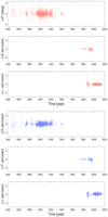 |
Fig. 2 O–C residuals for all types of observations during the period 1847–2016. |
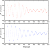 |
Fig. 3 Differences between our results and the Jacobson (2009) results in X (top panel) and Y (bottom panel) of Triton during the period 1847–2016. |
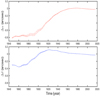 |
Fig. 4 Differences between our results and the Jacobson (2009) results in the right ascension (top panel) and declination (bottom panel) of Triton during the period 1847–2016. |
6 Conclusions
In this paper, a new numerical model of Triton’s motion is presented. Triton’s orbit is calculated using a numerical integrator, while the orientation of Neptune’s pole in particular is obtained by integrating the simplified Euler’s equations of motion. The parameters in the dynamical model are from Jacobson (2009). Our results regarding the orientation of Neptune’s pole are close to those from the Jacobson (2009) pole model. The differences are smaller than 2.5″. This method of calculating the pole’s motion could be used for estimating the related dynamical parameters to do further investigation of the Neptunian system.
The data for determining Triton’s orbit include 11 040 Earth-based observations from 1847 to 2016 and the Voyager 2 data. Our study included 1 306 new observations made during the period 2009–2016 when compared to the study by Jacobson (2009). The RMS of the residuals for the Earth-based CCD absolute observations are 0.102″ in right ascension and 0.142″ in declination.
The new orbit of Triton was calculated using the INPOP19a ephemeris. Our orbit is close to the orbit calculated by Jacobson (2009), who used the DE421 ephemeris. The differences are less than 0.02″ in relative positions X and Y during the period 1847–2016. The Voyager 2 data add a constraint on Triton’s orbit here. The high-precision ephemeris of Triton consistent with the INPOP ephemerides should be obtained together by adjusting the dynamical model.
Acknowledgements
We thank Dr Emelyanov for his advice on historical observations. This work is supported by the National Natural Science Foundation of China (Grant No.11803019 and 11703007) and the Scientific research project of Shanghai Science and Technology Commission (Grant No.19DZ1100500).
Appendix A Additional tables
Triton observation residuals (1847–1942).
Triton observation residuals (1975–2016).
References
- Aitken, R. G. 1899, Astron.Nachr., 149, 373 [Google Scholar]
- Aitken, R. G. 1904, Lick Observ. Bull., 51, 157 [CrossRef] [Google Scholar]
- Albrecht, S., & Smitil, E. 1909, Lick Observ. Bull., 5, 109 [NASA ADS] [CrossRef] [Google Scholar]
- Alden, H. L. 1940, AJ, 49, 70 [CrossRef] [Google Scholar]
- Alden, H. L. 1943, AJ, 50, 110 [CrossRef] [Google Scholar]
- Arlot, J. E., Dourneau, G., & Le Campion, J. F. 2008, A&A, 484, 869 [CrossRef] [EDP Sciences] [Google Scholar]
- Balanovskiĭ, I. A. 1923, Mitteilungen der Nikolai-Hauptsternwarte zu Pulkowo, 9, 85 [Google Scholar]
- Barnard, E. E. 1893, AJ, 13, 10 [CrossRef] [Google Scholar]
- Barnard, E. E. 1894, AJ, 14, 9 [CrossRef] [Google Scholar]
- Barnard, E. E. 1895, AJ, 15, 41 [CrossRef] [Google Scholar]
- Barnard, E. E. 1898, AJ, 19, 25 [CrossRef] [Google Scholar]
- Barnard, E. E. 1899, AJ, 20, 41 [CrossRef] [Google Scholar]
- Barnard, E. E. 1901, AJ, 22, 27 [CrossRef] [Google Scholar]
- Barnard, E. E. 1903, AJ, 23, 105 [CrossRef] [Google Scholar]
- Barnard, E. E. 1906a, AJ, 25, 41 [CrossRef] [Google Scholar]
- Barnard, E. E. 1906b, AJ, 25, 100 [CrossRef] [Google Scholar]
- Barnard, E. E. 1907, AJ, 25, 164 [CrossRef] [Google Scholar]
- Barnard, E. E. 1909, AJ, 181, 321 [Google Scholar]
- Barnard, E. E. 1910, AJ, 26, 144 [Google Scholar]
- Barnard, E. E. 1912, AJ, 27, 111 [Google Scholar]
- Barnard, E. E. 1913, AJ, 28, 10 [Google Scholar]
- Barnard, E. E. 1915, AJ, 29, 39 [Google Scholar]
- Barnard, E. E. 1916, AJ, 30, 2 [Google Scholar]
- Barnard, E. E. 1917, AJ, 30, 214 [Google Scholar]
- Barnard, E. E. 1919, AJ, 32, 103 [Google Scholar]
- Barnard, E. E. 1927, AJ, 37, 130 [Google Scholar]
- Bower, E. C., & Hall, A. 1923, AJ, 35, 108 [Google Scholar]
- Burton, H. E. 1913, AJ, 28, 44 [Google Scholar]
- Chanturia, S.M., & Kisseleva, T.P. 2006, Izvestiia glavnoi astronomicheskoi observatorii Pulkovo, 218, 188 [Google Scholar]
- Christie, W. H. M. 1901, Greenwich Observations in Astronomy, Magnetism and Meteorology made at the Royal Observatory, Series 2, 61, D240 [Google Scholar]
- Christie, W. H. M. 1904, Greenwich Observations in Astronomy, Magnetism and Meteorology made at the Royal Observatory, Series 2, 64, G59 [Google Scholar]
- Christie, W. H. M. 1909, Greenwich Observations in Astronomy, Magnetism and Meteorology made at the Royal Observatory, Series 2, 69, G207 [Google Scholar]
- Crawford, R. T. 1928, Lick Observ. Bull., 404, 8 [Google Scholar]
- Davis, C. H. 1874, MNRAS, 35, 49 [Google Scholar]
- Dinwiddie, W. W. 1903, AJ, 23, 144 [Google Scholar]
- Drew, D. A. 1897, AJ, 17, 131 [Google Scholar]
- Drew, D. A. 1899, AJ, 20, 30 [Google Scholar]
- Emel’Yanov, N. V., & Arlot, J.-E. 2008, A&A, 487, 759 [NASA ADS] [CrossRef] [EDP Sciences] [Google Scholar]
- Emelyanov, N. V., & Samorodov, M. Y. 2015, MNRAS, 454, 2205 [Google Scholar]
- Fienga, A., Deram, P., Viswanathan, V., et al. 2019, Notes Scientifiques et Techniques de l’Institut de Mecanique Celeste, 109 [Google Scholar]
- Folkner, W. M., Williams, J. G., Boggs, D. H., Park, R. S., & Kuchynka, P. 2014, Interplanet. Netw. Prog. Rep., 196, 1 [Google Scholar]
- Hammond, J. C. 1906, AJ, 25, 93 [Google Scholar]
- Hammond, J. C. 1908, AJ, 26, 18 [Google Scholar]
- Hammond, J. C., & Rice, H. L. 1905, AJ, 24, 188 [Google Scholar]
- Hall, A. 1876, Astron. Nachr., 88, 131 [Google Scholar]
- Hall, A. 1877, Astron. Nachr., 90, 161 [Google Scholar]
- Hall, A. 1900, AJ, 20, 191 [Google Scholar]
- Hall, A. 1911, AJ, 26, 179 [Google Scholar]
- Hall, A. 1920, AJ, 33, 62 [Google Scholar]
- Hall, A. 1922, AJ, 34, 18 [Google Scholar]
- Hall, A., & Burton, H. E. 1913, AJ, 28, 42 [Google Scholar]
- Hall, A., & Burton, H. E. 1919, AJ, 32, 113 [Google Scholar]
- Harrington, R. S., & Walker, R. L. 1984, AJ, 89, 889 [Google Scholar]
- Henry, P. 1884a, Bull. Astron., Ser. I, 1, 89 [Google Scholar]
- Henry, P. 1884b, Bull. Astron., Ser. I, 1, 178 [Google Scholar]
- Henry, P., Boinot, A., & Sy, F. 1886, Bull. Astron. Ser. I, 3, 488 [Google Scholar]
- Huang, T.-Y. 1990. Prog.Astron. 8, 222 [Google Scholar]
- Hussey, W. J. 1899, AJ, 20, 71 [Google Scholar]
- Hussey, W. J. 1902, Lick Observ. Bull., 17, 139 [Google Scholar]
- Jacobson, R. A. 1990, A&A, 231, 241 [Google Scholar]
- Jacobson, R. A. 1991, A&AS, 90, 541 [Google Scholar]
- Jacobson, R. A. 2009, AJ, 137, 4322 [Google Scholar]
- Jacobson, R. A., Riedel, J. E., & Taylor, A. H. 1991, A&A, 247, 565 [Google Scholar]
- Kostinsky, S. 1900, Astron. Nachr., 152, 277 [Google Scholar]
- Kostinsky, S. 1902, Astron. Nachr., 157, 287 [Google Scholar]
- Kulyk, I., Izakevich, E. M., & Shatokhina, S. 1990, Communication to the Natural Satellites Data Center [Google Scholar]
- Lassell, W. 1849a, MNRAS, 9, 103 [Google Scholar]
- Lassell, W. 1849b, MNRAS, 9, 221 [Google Scholar]
- Lassell, W. 1849c, MNRAS, 10, 8 [Google Scholar]
- Lassell, W. 1850, MNRAS, 10, 132 [Google Scholar]
- Lassell, W. 1851, MNRAS, 11, 61 [Google Scholar]
- Lassell, W. 1852a, MNRAS, 12, 155 [Google Scholar]
- Lassell, W. 1852b, MNRAS, 13, 37 [Google Scholar]
- Lassell, W. 1857, MNRAS, 17, 70 [Google Scholar]
- Lassell, W. 1864, MNRAS, 24, 209 [Google Scholar]
- Lohse, J. G. 1887, MNRAS, 47, 497 [Google Scholar]
- Masters, A., Achilleos, N., Agnor, C. B., et al. 2014, Planet. Space Sci., 104, 108 [Google Scholar]
- Neuĭmin, G. N., & Pokrovskiĭ, K. D. 1926, Mitteilungen der Nikolai-Hauptsternwarte zu Pulkowo, 10, 418 [Google Scholar]
- Owen, W.M. Jr. 1999, Communication to the Natural Satellites Data Center [Google Scholar]
- Owen W.M. Jr. 2001, Communication to the Natural Satellites Data Center [Google Scholar]
- Parrish, N. M., & Stone, O. 1892, AJ, 12, 90 [Google Scholar]
- Perrine, C. D. 1903, Lick Observ. Bull., 39, 70 [Google Scholar]
- Perrotin, H. J. 1887, Bull. Astron., Ser. I, 4, 339 [Google Scholar]
- Poroshina, A. L. 2013, Astron. Lett., 39, 876 [Google Scholar]
- Qiao, R. C., Yan, Y. R., Shen, K. X., et al. 2007, MNRAS, 376, 1707 [Google Scholar]
- Qiao, R. C., Zhang, H. Y., Dourneau, G., et al. 2014, MNRAS, 440, 3749 [Google Scholar]
- Royal Observatory Greenwich, 1899, MNRAS, 59, 501 [Google Scholar]
- Royal Observatory Greenwich, 1900, MNRAS, 61, 9 [Google Scholar]
- Royal Observatory Greenwich, 1903, MNRAS, 63, 503 [Google Scholar]
- Royal Observatory Greenwich, 1904, MNRAS, 64, 835 [Google Scholar]
- Royal Observatory Greenwich, 1905, MNRAS, 66, 10 [Google Scholar]
- Royal Observatory Greenwich, 1906, MNRAS, 67, 91 [Google Scholar]
- Royal Observatory Greenwich, 1907, MNRAS, 68, 33 [Google Scholar]
- Royal Observatory Greenwich, 1908, MNRAS, 68, 586 [Google Scholar]
- Royal Observatory Greenwich, 1913, MNRAS, 73, 155 [Google Scholar]
- Schaeberle, J. M. 1895, AJ, 15, 25 [Google Scholar]
- Schaeberle, J. M. 1897, AJ, 17, 62 [Google Scholar]
- Schaeberle, J. M. 1898, AJ, 18, 168 [Google Scholar]
- See, T. J. J. 1900, Astron. Nachr., 153, 257 [Google Scholar]
- Stone, R. C. 2000, AJ, 120, 2124 [Google Scholar]
- Stone, R. C. 2001, AJ, 122, 2723 [Google Scholar]
- Stone, R. C., & Harris, F. H. 2000, AJ, 119, 1985 [Google Scholar]
- Tapley, B., Schutz, B., & Born, G. H. 2004, Statistical Orbit Determination (Amsterdam: Elsevier) [Google Scholar]
- USNO 1875, Publ. U.S. Naval Observ. Second Ser., 13, 265 [Google Scholar]
- USNO 1881, Publ. U.S. Naval Observ., 17, 231 [Google Scholar]
- USNO 1911, Publ. U.S. Naval Observ. Second Ser., 6, A12 [Google Scholar]
- Veiga, C. H., & Vieira Martins, R. 1996, A&AS, 120, 107 [NASA ADS] [CrossRef] [EDP Sciences] [Google Scholar]
- Veiga, C. H., & Vieira Martins, R. 1998, A&AS, 131, 291 [NASA ADS] [CrossRef] [EDP Sciences] [Google Scholar]
- Vieira Martins, R., Veiga, C. H., Bourget, P., et al. 2004, A&A, 425, 1107 [NASA ADS] [CrossRef] [EDP Sciences] [Google Scholar]
- Viswanathan, V., Fienga, A., Gastineau, M., et al. 2017, Notes Scientifiques et Techniques de l’Institut de Mecanique Celeste, 108, 39 [Google Scholar]
- Walker, R. L., & Harrington, R. S. 1988, AJ, 95, 1562 [Google Scholar]
- Walker, R. L., Christy, J. W., & Harrington, R. S. 1978, AJ, 83, 838 [Google Scholar]
- Wang, N., Peng, Q. Y., Peng, H. W., et al. 2017, MNRAS, 468, 1415 [Google Scholar]
- Winlock, J., & Pickering, E. C. 1888, Annals of Harvard College Observatory, 13, 86 [Google Scholar]
- Wirtz, C. W. 1905, Astron. Nachr., 169, 33 [Google Scholar]
- Yan, D., Qiao,R. C., Cheng, X., et al. 2020, Icarus, 343, 113662 [Google Scholar]
- Young, C. A. 1888, AJ, 8, 14 [Google Scholar]
- Zhang, H. Y., Shen, K. X., Dourneau, G., et al. 2014, MNRAS, 438, 1663 [Google Scholar]
All Tables
Neptunian barycentric state vectors of Triton at Julian day (TDB) 2 447 763.5 (Aug. 25, 1989).
All Figures
|
Fig. 1 Differences in right ascension (top panel) and declination (bottom panel) of Neptune’s pole between our results and Jacobson (2009)’s results during the period 1847–2016. |
| In the text | |
|
Fig. 2 O–C residuals for all types of observations during the period 1847–2016. |
| In the text | |
|
Fig. 3 Differences between our results and the Jacobson (2009) results in X (top panel) and Y (bottom panel) of Triton during the period 1847–2016. |
| In the text | |
|
Fig. 4 Differences between our results and the Jacobson (2009) results in the right ascension (top panel) and declination (bottom panel) of Triton during the period 1847–2016. |
| In the text | |
Current usage metrics show cumulative count of Article Views (full-text article views including HTML views, PDF and ePub downloads, according to the available data) and Abstracts Views on Vision4Press platform.
Data correspond to usage on the plateform after 2015. The current usage metrics is available 48-96 hours after online publication and is updated daily on week days.
Initial download of the metrics may take a while.