| Issue |
A&A
Volume 641, September 2020
|
|
|---|---|---|
| Article Number | A48 | |
| Number of page(s) | 17 | |
| Section | The Sun and the Heliosphere | |
| DOI | https://doi.org/10.1051/0004-6361/202038220 | |
| Published online | 08 September 2020 | |
Nonlinear coupling of Alfvén and slow magnetoacoustic waves in partially ionized solar plasmas
1
Departament de Física, Universitat de les Illes Balears, 07122 Palma de Mallorca, Spain
e-mail: joseluis.ballester@uib.es
2
Departament de Ciències Matemàtiques i Informàtica, Universitat de les Illes Balears, 07122 Palma de Mallorca, Spain
3
Institute of Applied Computing & Community Code (IAC3), Universitat de les Illes Balears, Illes Balears, Spain
Received:
21
April
2020
Accepted:
17
June
2020
Context. Partially ionized plasmas constitute an essential ingredient of the solar atmosphere since layers such as the chromosphere and the photosphere and structures such as prominences and spicules are made of this plasma. On the other hand, ground- and space-based observations have indicated the presence of oscillations in partially ionized layers and structures of the solar atmosphere, which have been interpreted in terms of magnetohydrodynamic (MHD) waves.
Aims. Our aim is to study the temporal behavior of nonlinear Alfvén waves, and the subsequent excitation of field-aligned motions and perturbations, in a partially ionized plasma when dissipative mechanisms such as ambipolar diffusion, radiative losses, and thermal conduction are taken into account.
Methods. First, we applied the regular perturbations method for small-amplitude initial perturbations to obtain the temporal behavior of perturbations. Then we solved the full set of nonlinear MHD equations for larger values of the initial amplitude.
Results. We obtain analytical and numerical solutions to first-, second-, and third-order systems of equations and study the effects produced by ambipolar diffusion and thermal mechanisms on the temporal behavior of Alfvén and slow waves. We also study how the majority of the energy is transferred from the Alfvén waves to plasma internal energy. After numerically solving the full nonlinear equations when a large amplitude is assumed, the profile of the perturbations displays the typical sawtooth profile characteristic of associated shocks.
Conclusions. When ambipolar diffusion is taken into account, first-order Alfvén waves are damped in time, while second-order perturbations are undamped. However, due to the release of heat produced by ambipolar diffusion, other physical effects that modify the physical conditions in the spatial domain under consideration appear. On the other hand, the second-order perturbations are damped by thermal effects with a damping time that can be longer or shorter than that of Afvén waves. Therefore, after the initial excitation, Alfvén waves can be quickly damped, while slow waves remain in the plasma for a longer time, and vice versa.
Key words: magnetohydrodynamics (MHD) / Sun: filaments / prominences / Sun: oscillations
© ESO 2020
1. Introduction
Ground- and space-based observations have confirmed the presence of oscillatory motions in structures of the solar atmosphere, such as coronal loops and prominences. They have been interpreted in terms of standing or propagating magnetohydrodynamic (MHD) waves, opening the door to the development of coronal and prominence seismology. This approach seeks to obtain information about physical conditions in these coronal structures by comparing observations and theoretical models of oscillations. Reviews on these topics are available in Roberts et al. (1984), Roberts (2000, 2008), Aschwanden (2004), Nakariakov & Verwichte (2005), Nakariakov et al. (2016), Oliver (1999, 2009), Erdélyi & Goossens (2011), Ballester (2015), Arregui et al. (2018). In the case of solar prominences, they display various types of oscillatory motions; Oliver (1999) classified these oscillations into two categories based on velocity amplitude: small-amplitude events with amplitudes in the range of 3 − 10 km s−1, and large-amplitude events with amplitudes greater than 10 km s−1. These two categories represent truly different phenomena: small-amplitude oscillations are, in general, not related to flare activity and only affect a small volume of the prominence. On the other hand, large-amplitude oscillations are often associated with an energetic event that sets the full prominence (or a large part of it) into an oscillatory state (Luna et al. 2018). Hence, it is likely more accurate to speak of local versus global oscillatory events in prominences.
Alfvén waves are of paramount importance in laboratory plasma physics and astrophysics. In the case of solar physics, these waves have been used to explain how the energy flows through and heats the solar atmosphere; however, direct detection of these waves has proved to be difficult. In recent years, claims regarding the detection of these elusive Alfvén waves in different layers and structures of the solar atmosphere, such as sunspot umbra, bright-points, and spicules, have been made (Tomczyk et al. 2007; Jess et al. 2009; Mathioudakis et al. 2013; Srivastava et al. 2017; Grant et al. 2018; Kohutova et al. 2020). However, most of these reports are based on indirect signatures that have been interpreted in terms of Alfvén waves. From a theoretical point of view, linear Alfvén waves have been thoroughly studied (Cramer 2001; Mathioudakis et al. 2013) under the assumption of fully ionized plasmas. However, in recent years, studies of Alfvén waves in partially ionized plasmas have been developed. The main reason for this increased study is that these plasmas constitute an essential ingredient of the solar atmosphere, since many layers, such as the chromosphere and photosphere, and structures, such as prominences and spicules, are made of partially ionized plasmas (Zaqarashvili et al. 2012; Soler et al. 2015a,b, 2016; Cally & Khomenko 2018, 2019; González-Morales et al. 2019; Khomenko & Cally 2019).
The damping of Alfvén waves has been studied by different authors using different approaches. For instance, Leake et al. (2005) studied the damping of linear Alfvén waves due to collisions between neutrals and ions in a Vernazza, Avrett, Loeser (VALC) model (Vernazza et al. 1981) for the chromosphere using analytical and numerical methods. The study allowed the authors to determine which frequencies are completely damped and which are unaffected and allow for an undamped propagation of the waves. Song (2011) studied the heat released by strongly damped Alfvén waves in the solar corona. In this case, a two-fluid model (plasma and neutrals) was used and the damping was produced by self-consistently considering the collisions among electrons, ions, and neutrals, as well as the interaction between charged particles and the electromagnetic field. The authors applied this model to the chromosphere and the results indicate that lower frequencies are nearly undamped and can propagate through the atmosphere, while higher frequencies are strongly damped at low altitudes. Threlfall et al. (2011) studied the damping of Alfvén waves in the ion-cyclotron frequencies when the Hall term is taken into account and when uniform and non-uniform plasmas are considered. In the case of uniform plasmas, they used an analytical approach, while for non-uniform plasmas a numerical approach was needed. Finally, Lazarian (2016) investigated the effect of turbulence on the damping of Alfvén waves, which may have different astrophysical applications ranging from the launching of stellar and galactic winds to the propagation of cosmic rays in galaxies and clusters of galaxies.
Nonlinear Alfvén waves in fully ionized plasmas have also been a subject of study. It is well known that the behavior of a linearly polarized Alfvén wave depends on wave amplitude, and that in the case of large amplitudes these waves generate density perturbations and motions along the magnetic field lines. In this scenario a self-interaction appears, which is due to the ponderomotive force. Hollweg (1971) solved the equations for a linearly polarized Alfvén wave propagating parallel to the direction of the magnetic field in a perfectly conducting fluid up to second order in the wave quantities. In the second order, longitudinal wave velocity and density fluctuations appear to be driven by gradients in the wave magnetic pressure. The main conclusions were: in the low β regime, large-amplitude linearly polarized Alfvén waves also have longitudinal motions and density fluctuations associated with them; and the Alfvén wave magnetic field and transverse velocity are not affected by second-order effects, but are affected by third-order terms, which were neglected. Rankin et al. (1994) and Tikhonchuk et al. (1995) investigated the nonlinear dynamics of standing shear Alfvén waves in cold magnetized plasmas. First, and in the limit β = 0, they obtained analytical approximations for second-order longitudinal velocity and density perturbations, corresponding to slow waves, as well as analytical approximations for third-order Alfvén wave quantities. In the second order, they found a secularly growing temporal behavior for longitudinal velocity and density perturbations; this produces a density enhancement at the velocity antinodes of Alfvén waves and a depletion near the nodes, with an angular frequency equal to 2kzcs, where cs is the sound speed, and an effective wavenumber of 2kz, where kz is the longitudinal wavenumber of the Alfvén wave. When the assumption of β = 0 is removed, the secular effects on longitudinal velocity and density perturbations disappear and periodic behaviors are found. Finally, they derived third-order analytical approximations and used numerical solutions to the full set of nonlinear ideal MHD equations to test the validity of analytical results. Verwichte et al. (1999) studied the temporal evolution of Alfvénic pulses in cold homogeneous plasmas. The initial disturbance produces two pulses traveling in opposite directions; the ponderomotive force of the two pulses produces a static shock in longitudinal velocity at the initial position, while the traveling pulses form a shock described by a Cohen-Kulsrud equation. They found a good agreement between the derived analytical solutions and the numerical results. Terradas & Ofman (2004) studied the effect of large-amplitude waves in loops as a possible mechanism to produce density enhancements at loop tops due to the effect of the ponderomotive force of standing waves. They solved the nonlinear three-dimensional MHD equations in a flux tube configuration and found that for large initial perturbations a pressure imbalance appears along the loop, producing upflows from the footpoints. Therefore, the accumulation of mass at the loop top produces a significant density enhancement. Thurgood & McLaughlin (2013) numerically investigated the effects of ponderomotive force induced by Alfvén waves in inhomogeneous 2.5D MHD plasmas. They analysed the source terms in the nonlinear wave equations when the magnetic field and density are inhomogeneous; they conclude that the ponderomotive effects are induced by any Alfvén wave propagating in any medium and may affect the dynamics of energy transport and aspects of dissipation. Zheng et al. (2016) studied the effects of dissipative mechanisms, such as resistivity and viscosity, on nonlinear Alfvén wave trains. In weakly dissipative one-dimensional systems, the main effect is the damping of Alfvén waves and the heating of plasma; however, in the case of strong dissipation, the Alfvén wave train develops a damped soliton. In two-dimensional systems, phase mixing is present, which enhances damping and plasma heating. Finally, Lardner & Trehan (1991) studied the nonlinear evolution of Alfvén and magnetoacoustic waves in a low-density plasma with a strong magnetic field, using a very different approach based on the Chew-Goldberger-Low approximation. In the reported research on nonlinear Alfvén waves, the plasma has always been considered as fully ionized and treated as a single fluid. This assumption of fully ionized plasma is valid, for instance, for the solar corona; however, as we have previously pointed out, the plasma is only partially ionized in some layers and structures of the solar atmosphere. On the other hand, except in one case (Zheng et al. 2016), dissipative effects have not been taken into account, and ideal or resistive MHD equations have been used. Therefore, it is of great interest to study the behavior of nonlinear Alfvén waves in partially ionized plasmas; this approach was taken by Martínez-Gómez et al. (2018), who, using a nonlinear multi-fluid code, investigated the behavior of high-frequency nonlinear waves in a partially ionized plasma, paying special attention to the heating caused by ion-neutral collisions.
The aim of this paper is to study the temporal behavior of nonlinear Alfvén waves in a partially ionized plasma, whose physical conditions are those of quiescent solar prominences, when ambipolar diffusion is taken into account. For this study, we consider our plasma as a single fluid and, apart from ambipolar diffusion, we have also included radiative losses and thermal conduction as dissipative mechanisms for the field-aligned motions and density perturbations excited in the plasma by the ponderomotive force. Furthermore, third-order Alfvén waves, which are influenced by these second-order perturbations which in turn are influenced by thermal effects, have also been studied.
The layout of the paper is as follows: First we introduce single-fluid MHD equations, an equilibrium model and dissipative mechanisms; next, we derive equations for parallel propagating waves and apply the regular perturbations method, obtaining first-, second-, and third-order equations which have been solved for different cases; finally, we obtain numerical solutions for the full set of nonlinear MHD equations and compare the results with those from the regular perturbations approach.
2. Basic equations
2.1. Governing equations in the single-fluid approximation
We study the dynamics of partially ionized plasmas within the framework of the single-fluid approximation. In short, the single-fluid approximation assumes a strong coupling between ions, electrons, and neutrals so that all the species effectively behave as one fluid. In this approximation, the basic MHD equations are written in terms of total quantities, while the effect of the interactions between the various species remains in the form of several nonideal terms. For instance, the influence of ion-neutral collisions is present through the so-called ambipolar diffusion effect, which acts as a diffusive mechanism for the magnetic field. The single-fluid approximation is appropriate when studying MHD waves in partially ionized plasmas as long as the wave frequency remains lower than the ion-neutral collision frequency. The values of the collision frequencies in the solar chromosphere can be checked, for example, in Fig. 11 of Ballester et al. (2018); in solar prominences, the collision frequencies are similar to those found in the upper chromosphere. In the following expressions, MKS units have been used.
The basic single-fluid equations used in this work are:
![$$ \begin{aligned}&\frac{\partial \boldsymbol{B}}{\partial t} = \nabla \times \left( \boldsymbol{v}\times \boldsymbol{B}\right) - \nabla \times \left( \eta \nabla \times \boldsymbol{B}\right)\nonumber \\&\qquad + \nabla \times \left\{ \eta _{\rm A}\left[ \left( \nabla \times \boldsymbol{B}\right) \times \boldsymbol{B}\right] \times \boldsymbol{B}\right\} , \end{aligned} $$](/articles/aa/full_html/2020/09/aa38220-20/aa38220-20-eq3.gif)

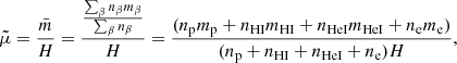
where  denotes the material or total derivative, ρ is the mass density, p is the thermal pressure, T is the temperature, v is the velocity vector, B is the magnetic field vector, γ is the adiabatic index, μ the magnetic permeability, η and ηA are the coefficients of Ohmic and ambipolar diffusion, respectively, ℒ represents the net effect of all the sources and sinks of energy, R is the gas constant, and
  is the mean molecular weight. Equations (1)–(5) are the continuity, momentum, induction, energy, and state equations, respectively.
2.2. Ionization state
The ionization state of the plasma is determined by the balance between ionization and recombination. The general approach to computing the ionization state is to take into account all the ionization and recombination processes and to determine the time-dependent values of the ionized and neutral fractions. Here, to estimate the ionization degree, we follow Heinzel et al. (2015), who used one-dimensional non-LTE radiative transfer models (Heinzel et al. 2014) to determine the ionization degree in several prominence slabs. In particular, these authors provide tables for the ionization degree for different temperatures and pressures at the prominence. Heinzel et al. (2015) consider a prominence plasma composed of hydrogen and helium, whose abundance is 10% and which is fully neutral. Then, the ionization degree i is defined as  , where ne is the electron density number and nH is the total hydrogen density number (nH I + np), using the following subscripts: e for electrons, p for protons, H for neutral hydrogen plus protons, HI for neutral hydrogen, and HeI for neutral helium; the total particle density number is N = nH + nHe I +ne. Then, taking into account that nHe| I = 0.1nH, N can be written as
and the gas pressure, p = NkBT, is given as
or, using the mass density, as
where kB is the Boltzmann constant and H is the atomic mass unit. Using Table 1 in Heinzel et al. (2015) and the Fit function from the Mathematica symbolic package, we performed a polynomial fit, up to the third order in pressure p and temperature T as well as product terms and interactions, of the ionization degree:

where a, b, c, d, e, f, g, h, j, and k are the coefficients of the fitted function (see Appendix A). Then, using Eq. (9) together with the temperature and pressure values in Heinzel et al. (2015), we can compute the fitted ionization degree. The goodness of our surface fitting is assessed by computing the determination coefficient R2:
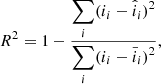
where ii corresponds to the values of the ionization degree in Heinzel et al. (2015),  corresponds to the fitted ionization degree using Eq. (9), and
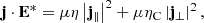
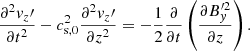
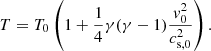
  corresponds to the mean of the values of the ionization degree in Heinzel et al. (2015). Using Eq. (10), the obtained value for R2 is 0.98 or 98%. Figure 1 compares the fitted surface, described by Eq. (9), to data in Table 1 of Heinzel et al. (2015), visually showing the goodness of the fit.
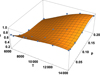 |
Fig. 1. Ionization degree i versus temperature T and pressure p. The blue dots correspond to data in Table 1 in Heinzel et al. (2015); the surface represents the fitting described by Eq. (9). |
Next, in order to determine the total particle density number we need to know the plasma pressure; from Eq. (8), the ionization degree can be written as
Then, once a value for the density was assumed, and using the different temperature values in the Heinzel et al. (2015) table, we solved Eqs. (9) and (11) together. When the pressure is determined, the total particle density number is obtained from

and the rest of particle density numbers can be determined from


Finally, the mean molecular weight can be computed as
where  is the mean mass per particle.
2.3. Dissipative mechanisms
The induction equation (Eq. (3)) contains two magnetic diffusion terms in addition to the ideal convective term. The second term on the right-hand side is Ohmic diffusion, which is caused by electron collisions. The coefficient of Ohmic diffusion is given by

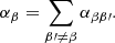
where e is the electron charge. The total friction coefficient of species β with other species is
Therefore, in our case, the total friction coefficient of electrons αe with protons, neutral hydrogen, and neutral helium is

The friction coefficient for collisions between two charged species q and q′ (Spitzer 1962; Braginskii 1965) is
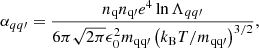
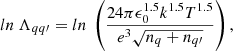
where mqq′ = mqmq′/(mq+mq′) is the reduced mass, ϵ0 is the permittivity of free space, and lnΛqq′ is the Coulomb’s logarithm (Spitzer 1962; Vranjes & Krstic 2013). This logarithm is given by
while the friction coefficient for collisions between a charged or neutral species β = e, p, H I, He I, and neutral species n = H I, He I is
![$$ \begin{aligned} \alpha _{\beta n} = m_{\beta } n_{n} m_{\beta n} \left[\frac{8 k T}{\pi m_{\beta n}}\right]^{1/2} \sigma _{\beta n} , \end{aligned} $$](/articles/aa/full_html/2020/09/aa38220-20/aa38220-20-eq29.gif)
where σβn is the collision cross section (Vranjes & Krstic 2013).
The third term on the right-hand side of Eq. (3) is ambipolar diffusion. This term contains the effect of ion-neutral collisions in the single-fluid approximation. The coefficient of ambipolar diffusion in a hydrogen-helium plasma (Zaqarashvili et al. 2013) is
with the friction coefficients for αHeI and αHI given by


The effect of all the sources and sinks of energy is included in the function ℒ on the right-hand side of the energy equation (Eq. (4)). The expression of ℒ is

where the various terms on the right-hand side are the heat flux due to thermal conduction ∇ ⋅ (κ∇T). Here, κ is the thermal conductivity tensor and L(ρ,T) is the radiative loss function. The j ⋅ E* is the generalized Joule heating, where  is the current density and E* is the effective electric field. The h represents an additional and unspecified external constant heating per unit volume. The thermal conduction in a magnetized plasma is strongly anisotropic. For convenience, we split the thermal conduction term in Eq. (27) into its components that are parallel and perpendicular to the magnetic field direction, namely

where κ∥ and κ⊥ are the parallel and perpendicular conductivities, respectively, with respect to the magnetic field direction, and |B|2 is the square of the modulus of the magnetic field vector. In a fully ionized plasma, κ∥ is essentially determined by the electron conductivity, while κ⊥ is mainly determined by ions. In a partially ionized plasma, the isotropic conductivity of neutrals has to be added to both parallel and perpendicular components. Thus, the parallel and perpendicular components of thermal conductivity are approximated by κ∥ ≈ κe, ∥ + κn and κ⊥ ≈ κn, where κe, ∥ and κn are the parallel electron thermal conductivity and the total neutral thermal conductivity, respectively, as given by (Braginskii 1965; Meier 2011; Soler et al. 2015a):
where αβ, tot is the total friction coefficient of species β, given by αβ, tot = αβ + αββ; this includes the term αββ, which accounts for self-collisions.
The radiative loss function, L(ρ,T), accounts for radiative losses due to plasma cooling. Determining the plasma radiative losses as a function of temperature and density is a difficult task that requires complicated numerical solutions of the radiative transfer problem. The radiative loss rate depends, for example, on the completeness of the atomic model used for the calculation, on the atomic processes included, on the ionization equilibrium, and on the assumed element abundance, among other factors. The solution of the radiative transfer problem is beyond the scope of the present paper. A frequent alternative approach to account for the plasma radiative losses is to use semi-empirical parametrizations of the radiative loss function that are widely available in the literature (Rosner et al. 1978; Milne et al. 1979; Dahlburg & Mariska 1988; Klimchuk & Cargill 2001; Carbonell et al. 2004; Landi et al. 2012). These parametrizations enable us to incorporate radiative losses in a consistent way without needing to solve the full radiative transfer problem. The expression of the radiative loss function we used is
where χ* and α are piecewise constants dependant on the temperature, and we use the parametrization of χ* and α given in Hildner (1974) (see Table 1). The inconvenience of this approach is that the semi-empirical radiative loss function is obtained under the assumption of optically thin plasma, while the cool partially ionized plasmas of interest here may not completely satisfy this condition. Owing to finite optical thickness, the actual radiative losses of the plasma would probably be reduced to some degree compared to the optically thin calculation.
Numerical values of the piecewise constants χ* and α for prominences (Hildner 1974).
Finally, the generalized Joule heating j ⋅ E* takes into account plasma heating due to the dissipation of electric currents by both Ohmic and ambipolar diffusion. The expression of j ⋅ E* is
where ηC is the so-called Cowling’s (or total) diffusivity given by
and j∥ and j⊥ are the components of the current density parallel and perpendicular to the magnetic field, respectively, that can be computed as
![$$ \begin{aligned}&\mathbf{j}_\parallel = \frac{1}{\mu } \frac{\left[ \left( \nabla \times \boldsymbol{B}\right) \cdot \boldsymbol{B}\right] \boldsymbol{B}}{\left| \boldsymbol{B}\right|^2} \end{aligned} $$](/articles/aa/full_html/2020/09/aa38220-20/aa38220-20-eq41.gif)
![$$ \begin{aligned}&\mathbf{j}_\perp = \frac{1}{\mu } \frac{\boldsymbol{B}\times \left[ \left( \nabla \times \boldsymbol{B}\right) \times \boldsymbol{B}\right]}{\left| \boldsymbol{B}\right|^2}\cdot \end{aligned} $$](/articles/aa/full_html/2020/09/aa38220-20/aa38220-20-eq42.gif)
Thus, Ohmic diffusion is responsible for the dissipation of parallel currents, while Cowling’s diffusion, that is to say the joint effect of Ohmic and ambipolar diffusion, is responsible for the dissipation of perpendicular currents.
2.4. Equations for parallel-propagating waves
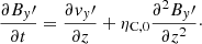
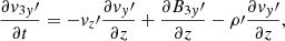
We use a Cartesian coordinate system and assume that the plasma properties vary on the z-direction only, whereas x and y are ignorable directions. Then, we can conveniently rotate the coordinate system for v and B to lie on the zy-plane with no loss of generality. Hence, v = (0, vy, vz) and B = (0, By, Bz). The solenoidal condition ∇ ⋅ B = 0 imposes that ∂Bz/∂z = 0, while from the z-component of Eq. (3) we get ∂Bz/∂t = 0. Therefore, Bz is a constant in both space and time. In this one-dimensional case, Eqs. (1)–(4) become
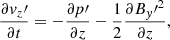
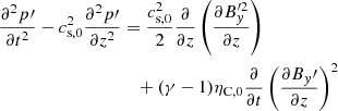
![$$ \begin{aligned}&\frac{\partial p}{\partial t} = - { v}_z \frac{\partial p}{\partial z} - \gamma p \frac{\partial { v}_z}{\partial z} \nonumber \\&\qquad + \left(\gamma -1 \right) \left[ \frac{1}{\mu }\eta _{\rm C}\left( \frac{\partial B_{ y}}{\partial z} \right)^2 + \frac{\partial }{\partial z}\left(\frac{B_z^2 \kappa _\parallel + B_{ y}^2 \kappa _\perp }{B_z^2 + B_{ y}^2} \frac{\partial T}{\partial x} \right)\right]\nonumber \\&\qquad - \left(\gamma -1 \right) \left(\rho ^2 \chi ^* T^\alpha - \rho h \right) , \end{aligned} $$](/articles/aa/full_html/2020/09/aa38220-20/aa38220-20-eq47.gif)
3. Regular perturbations approach
Before exploring the numerical solutions to Eqs. (36)–(40), we perform an approximate analytic study of the solutions in the limit of small amplitudes in this section. To do so, we consider small-amplitude Alfvén waves superimposed on a homogeneous and constant equilibrium state. The purpose of this section is to establish an analytic basis that can be compared to the fully numerical simulations performed later. We define the parameter ϵ ≡ v0/cA, 0, where v0 is the Alfvén wave initial velocity amplitude and cA, 0 is the equilibrium Alfvén speed. Then, assuming that ϵ ≪ 1, we write


where the subscript 0 denotes a homogeneous and constant equilibrium quantity and the prime ′ denotes a perturbation. Since, initially, we are interested in Alfvén waves, the perturbations of the perpendicular components of velocity and magnetic field are assumed to be of first order in ϵ with a third-order correction, while the perturbations of the remaining quantities are assumed to be second order in ϵ. Contributions with higher orders in ϵ are neglected. We substitute these quantities in Eqs. (36)–(40) and separate the various terms according to their order with respect to ϵ. From the zeroth order equations in ϵ, we find that the unspecified external heating source must be  to compensate for radiative losses in order for the equilibrium to be satisfied. The first-order equations in ϵ govern the behavior of
  and
and  , and so they describe linear Alfvén waves. The second-order equations in ϵ involve
  , p′, ρ′, and T′, so that they describe the generation of slow magnetoacoustic waves due to the nonlinear coupling with the Alfvén waves. The equations for higher orders in ϵ represent nonlinear corrections on the Alfvén and slow waves. In this approximate study, we restrict ourselves to the first-, second-, and third-order equations in ϵ.
3.1. First-order equations
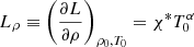
In order to write all the equations under study in dimensionless forms, we introduce the following dimensionless quantities:
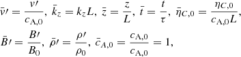
where L corresponds to half the size of the spatial domain under consideration and τ is a characteristic timescale, which are related through the equilibrium Alfvén speed cA,0 = L/τ. Hereafter we drop bars for the sake of simplicity.
The first-order equations in ϵ are:

These two equations involve the components of v and B transverse to the equilibrium magnetic field and can appropriately be combined into an equation for  only, namely
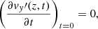
where ηC,0 is Cowling’s diffusivity computed at the equilibrium state. Equation (51) governs linear Alfvén waves that are damped by ambipolar and Ohm’s diffusion, and it can also be shown that  satisfies a similar equation. Since we are interested in an analytical solution to Eq. (51) describing damped linear standing Alfvén waves, we use the separation of variables method. We assume that
  (z, t) can be written as
Then, substituting this expression in Eq. (51) and using  as the separation constant, we obtain
where the separation constant kz plays the role of the wavenumber along the magnetic field direction. Assuming the stationary state of wave propagation, the solution to Eq. (53) can be obtained assuming that g(t) behaves harmonically as eiωt, which provides a dispersion relation of
whose solution for ω is
a complex angular frequency, ω = ωr + iωi, with

Then, g(t) can be written as

On the other hand, the solution to Eq. (54) is

Then,  (z, t) can be written as
Now, in order to determine the four constants of integration, we impose the following conditions representative of a standing oscillation with wavelength equal to 4L:
where the longitudinal wavenumber  , and v0 is the initial amplitude. Then, using the above conditions, the final solution for the transverse velocity perturbation is
![$$ \begin{aligned}&{ v}_{ y}\prime (z,t) = { v}_0 \exp \left[-\frac{1}{2} k_z^2 \eta _{\rm C,0}t \right] \left(\cos \ \omega _r \ t + \frac{k_z^2 \eta _{\rm C,0}}{2 \omega _r} \sin \ \omega _r \ t \right) \times \cos \ k_z z \end{aligned} $$](/articles/aa/full_html/2020/09/aa38220-20/aa38220-20-eq83.gif)
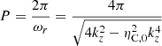
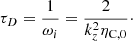
with the period and damping time given by
Once the expression for the perturbed velocity amplitude is known, the solution for the perturbed magnetic field  can be obtained by integrating

to obtain
![$$ \begin{aligned} B_{ y}\prime (z,t) =\frac{{ v}_0 \exp \left[-\frac{1}{2} k_z^2 \eta _{C,0} t \right] (k_z^4 \eta _{\rm C,0}^2+4 \omega _r^2) \sin \ k_z z \ \sin \ \omega _r t}{4 k_z \omega _r} .\end{aligned} $$](/articles/aa/full_html/2020/09/aa38220-20/aa38220-20-eq88.gif)
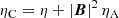
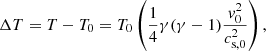
In order to plot the temporal behavior of first-order perturbed velocity and magnetic fields, we impose the dimensionless initial amplitude of the velocity perturbation v0 = 0.15 and compute other dimensionless quantities such as ηC,0 and ωr. To this end, we assume values for the magnetic field, density, and temperature typical of quiescent prominences B0 = 5 × 10⁻⁴ T, ρ0 = 5 × 10⁻¹¹ kg ⋅ m−3, and T = 12 000 K. Then, using these values, the Alfvén speed, cA,0, is 63.08 km s−1 and the sound speed, cs,0, is 15.08 km s−1. Furthermore, in order to remain in the low-frequency regime and to satisfy the requirements of single-fluid approximation, we take L = 106 m as our characteristic length and τ = 15.85 s is our characteristic timescale; these values give a period for the Alfvén waves of 64.35 s and a frequency of 0.015 Hz. Finally, using Eq. (48), our dimensionless quantities are ηC,0 = 0.0023 and ωr = 1.57. The temporal behavior of the linear Alfvén velocity and magnetic field perturbations can be seen in Fig. 2, which shows the damping of the linear Alfvén wave produced by ambipolar diffusion.
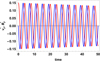 |
Fig. 2. Dimensionless linear Alfvén wave velocity (red) and magnetic field perturbations (blue) versus dimensionless time. The velocity amplitude has been computed at z = 0, while the magnetic field amplitude has been computed at z = 1 (T = 12 000, v0 = 0.15, kz = π/2, ηC,0 = 0.0023). |
3.2. Second-order equations
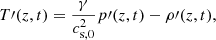
The second-order equation in ϵ corresponding to the energy equation (Eq. 40) is
![$$ \begin{aligned} \frac{\partial p\prime }{\partial t}&= - \gamma p_0 \frac{\partial { v}_z\prime }{\partial z} + \left(\gamma -1 \right) \left[ {\kappa _{\parallel ,0}} \frac{\partial ^2 T\prime }{\partial z^2} - \rho _0 \left( L_\rho \rho \prime + L_T T\prime \right)\right] \nonumber \\&\quad + \left(\gamma -1 \right)\left[\frac{1}{\mu _0}\eta _{\rm C,0}\left(\frac{\partial {B_{ y}\prime }}{\partial z}\right)^2 \right], \end{aligned} $$](/articles/aa/full_html/2020/09/aa38220-20/aa38220-20-eq89.gif)
where κ∥, 0 denotes the value of κ∥ computed with the equilibrium quantities (see Sect. 2.3), and Lρ and LT are the partial derivatives of the radiative loss function with respect to density and temperature, respectively, evaluated at the equilibrium state, namely

In addition, p′, ρ′, and T′ are related through the perturbed equation of state as
where the term of order ϵ4 has been neglected. In writing this last equation, we assumed, for the sake of simplicity, that the ionization degree of the plasma remains approximately constant. Now, we introduce
In order to obtain the dimensionless energy equation, we introduce the following dimensionless quantities:
Then, the dimensionless second-order equations become

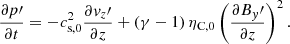
![$$ \begin{aligned} \frac{\partial p\prime }{\partial t}&= - c_{\mathrm{s,0} }^2 \frac{\partial { v}_z\prime }{\partial z} + \left(\gamma -1 \right) \left[ {\kappa _{\parallel ,0}} \frac{\partial ^2 (p\prime - \frac{c_{\mathrm{s,0} }^2}{\gamma } \rho \prime )}{\partial z^2}\right] \nonumber \\&\quad - \left(\gamma -1 \right) \left[\frac{c_{\mathrm{s,0} }^2}{\gamma } \left( \omega _\rho \rho \prime + \omega _T \left(\frac{\gamma }{c_{\mathrm{s,0} }^2} p\prime -\rho \prime \right) \right)\right] \nonumber \\&\quad + \left(\gamma -1 \right)\eta _{\rm C,0}\left(\frac{\partial {B_{ y}\prime }}{\partial z}\right)^2, \end{aligned} $$](/articles/aa/full_html/2020/09/aa38220-20/aa38220-20-eq97.gif)
where αωρ = ωT and, using Eqs. (74), (48), and (76), T′ has been written as
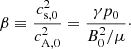
which has been substituted in Eq. (79). The right-hand side of Eq. (78) involves a quadratic term in  , which drives slow magnetoacoustic waves, since the second-order magnetic pressure perturbation associated with the Alfvén waves couples with the thermal pressure perturbation associated with the slow waves. In absence of this term and the last term in Eq. (79), Eqs. (77)–(79) would represent free slow magnetoacoustic waves damped by thermal conduction and radiative losses. Here we are not interested in the free slow waves, which have been described elsewhere (Goossens 2003; Roberts 2004, 2006; Priest 2014). Instead, we focus on the solution that represents the generation of slow magnetoacoustic waves due to the nonlinear coupling with the Alfvén waves. On the other hand, from here on it is assumed that
  ; that is to say, we consider a low-β plasma, where the plasma β is defined as
In the following subsections, we consider different cases in order to understand how the involved physical mechanisms affect the temporal behavior of second-order perturbations.
3.2.1. Case where radiation and thermal conduction are neglected
First, we consider the case in which radiation and thermal conduction are neglected. We assume an equilibrium temperature of T = 12 000 K and, following Sect. 2.1, the ionization degree in this case is i = 0.82, the mean molecular weight is  , and β = 0.07. From Eqs. (77)–(79), the system of equations to be solved is


In this system of equations, the only dissipative term is the second term on the right-hand side of Eq. (84), where the expression for  obtained from Eq. (70) has been used. The system of equations was solved, numerically, together with the following initial and boundary conditions, respectively,

The case without ambipolar diffusion was studied by Rankin et al. (1994) and Tikhonchuk et al. (1995), among others. To recover it we can neglect the dissipative term in Eq. (84) and combine the remaining equations to obtain a partial differential equation for the longitudinal velocity perturbation,  ,
,
Using the D’Alembert’s method, an analytical solution to this equation can be found, namely
![$$ \begin{aligned} { v}_z\prime = \frac{{ v}_0^2 \omega _r^3 sin \ ( 2 k_z z) \left[\omega _r \ sin \ (2 c_{\mathrm{s,0} }k_z t) - c_{\mathrm{s,0} }k_z sin \ (2 \omega _r t )\right]}{( 8 c_{\mathrm{s,0} }^3 k_z^4 - 8 c_{\mathrm{s,0} }k_z^2 \omega _r^2)}\cdot \end{aligned} $$](/articles/aa/full_html/2020/09/aa38220-20/aa38220-20-eq110.gif)
This analytical solution can be decomposed in two sinusoidal terms with angular frequencies 2cs,0kz and 2ωr, respectively; the longitudinal velocity perturbation comes from the composition of the two sinusoidal curves with different amplitudes and angular frequencies. Considering the low β regime, cs,0kz ≪ ωr, the second term in Eq. (87) can thus be neglected and the dominant angular frequency of the solution is 2cs,0kz (Rankin et al. 1994; Tikhonchuk et al. 1995). Using the already known value for cs,0, the oscillatory period is 132 s, although this value is an approximation to the true period.
To explore the effect of ambipolar diffusion produced by a change of the Alfvén wave wavelength, we consider the following values for L: 107 m, 105 m, and 5 × 10⁴ m; therefore, the corresponding wavelengths are 4 × 10⁷ m, 4 × 10⁵ m, and 2 × 10⁵ m. Using these values for L, three different values for the dimensionless Cowling’s coefficient are obtained, 0.00023, 0.023, and 0.045, respectively, which have been used when numerically solving Eqs. (82)–(84).
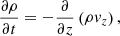
Figure 3 shows the temporal and spatial behavior of the heat released due to ambipolar diffusion. We observe that most of the heat is released at the central part of the spatial domain and decreases towards the boundaries, and that it is attenuated in time, as can be expected. When different values of Cowling’s diffusivity are considered, we find that the amount of heat released increases when Cowling’s diffusivity is increased.
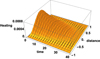 |
Fig. 3. Dimensionless heating versus dimensionless time and space for ηC,0 = 0.023. |
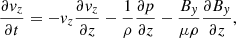
Figure 4 displays the temporal behavior of pressure perturbation at z = 0 (left panel) and z = 1 (right panel) for the different values of Cowling’s diffusivity that are considered. At the center (z = 0) of the spatial domain, pressure perturbations are always positive and the amplitude increases when Cowling’s diffusivity is increased. However, for the smallest considered value of Cowling’s diffusivity, pressure perturbations become very slightly negative at the minimum of the oscillations. It seems that the net effect of an increase in Cowling’s diffusivity is that pressure perturbation curves within the positive zone of the plot are slightly shifted up, while a decrease produces a downward shift of the curves, which slightly enter the negative zone of the plot, as can be observed in Fig. 4 (left panel). At the boundary (z = 1) of the spatial domain, we observe two different behaviors: for the highest and the intermediate values of Cowling’s diffusivity, the amplitude of the pressure perturbation goes from negative to positive values, while for the smallest value of Cowling’s diffusivity, the amplitude of the pressure perturbation is negative. This behavior of pressure perturbations is directly related to the behavior of density and temperature perturbations. In the case of density perturbations (Fig. 5), they become negative at the center (z = 0) of the spatial domain for any significant value of Cowling’s diffusivity, while they become positive at the boundary (z = 1). A similar behavior is observed in Fig. 6 for temperature perturbations; we note the sudden increase of the temperature perturbation during the time in which most of the heating is released (Fig. 6, left panel). We also observe that, as expected, as the value of Cowling’s diffusivity increases, so does the temperature perturbation because of the more intense heating. Once the initial temperature increase is over, the temperature perturbations become oscillatory in the same way the pressure and density perturbations do. On the contrary, at z = 1 (Fig. 6, right panel) we only observe oscillatory perturbations without, as before, any sudden increase in temperature due to the lack of heat released at the boundaries of the spatial domain. During the oscillatory behavior, whose amplitude becomes constant after some time, the observed temperature variations are due to the interplay between pressure and density perturbations shown in Eq. (80). Finally, Fig. 7 (left panel) displays the temporal behavior of longitudinal velocity perturbations, at z = 0.5, for the three different values of Cowling’s diffusivity. It is interesting to note that the high-frequency distortions of the sinusoidal shape that appear for the very low value of ηC,0 disappear when the value of ηC,0 is increased. Therefore, a sufficiently intense Cowling’s diffusion is able to damp the high-frequency modulation of the longitudinal velocity perturbation, which is associated with the damped Alfvén wave. Only the low frequency, associated with the slow wave, remains.
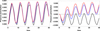 |
Fig. 4. Dimensionless pressure perturbations versus dimensionless time computed at z = 0 (left) and z = 1 (right), for ηC,0 = 0.00023 (black), 0.023 (blue), and 0.045 (red). |
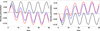 |
Fig. 5. Dimensionless density perturbations versus dimensionless time computed at z = 0 (left) and z = 1 (right), for ηC,0 = 0.00023 (black), 0.023 (blue), and 0.045 (red). |
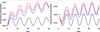 |
Fig. 6. Dimensionless temperature perturbations versus dimensionless time computed at z = 0 (left) and z = 1 (right), for ηC,0 = 0.00023 (black), 0.023 (blue), and 0.045 (red). |
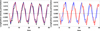 |
Fig. 7. Left panel: dimensionless longitudinal velocity perturbations versus dimensionless time computed for ηC,0 = 0.00023 (black), 0.023 (blue), and 0.045 (red); Right panel: dimensionless longitudinal velocity perturbation versus dimensionless time. Full analytical solution obtained from Eq. (89) (red) and numerical solution (blue) (z = 0.5, v0 = 0.15, kz = π/2, ηC,0 = 0.045 and 0.00023). |
The temporal behavior of pressure, density, and temperature perturbations can be understood as follows. For any significant value of Cowling’s diffusivity, the release of heat due to ambipolar diffusion produces, for short periods, an increment of temperature around the center of the spatial domain. Later on, the behavior of the temperature becomes oscillatory. The rise in temperature at the center of the spatial domain, because of the heating, causes a local increment of pressure. In turn, this over-pressure pushes the material away from the center, so that a longitudinal flow towards the boundaries is generated. As a result of this, mass density decreases at the center and increases near the boundaries (see Fig. 8). We note that this effect is the opposite of that of the ponderomotive force, which tends to accumulate mass at the center of the domain. Which of the two effects dominates depends on the efficiency of the heating due to ambipolar diffusion.
 |
Fig. 8. Dimensionless density perturbation versus dimensionless time and space for ηC,0 = 0.045. |
On the other hand, Eqs. (82)–(84) can be combined to obtain the following wave equations:
Then, analytical solutions for pressure (p′) and longitudinal velocity perturbations ( ) can be found by means of D’Alembert’s method, and for density perturbations (ρ′) from Eq. (82). These solutions are much more complex than in the case without ambipolar diffusion (Eq. (87)) and are not shown here. Instead, in Fig. 7 (right panel), we compare the obtained analytical solution for velocity perturbation with the previously obtained numerical solution for two different values of Cowling’s diffusivity and find a perfect agreement.
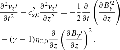
These full analytical solutions for the pressure, longitudinal velocity, and density perturbations obtained from Eqs. (88), (89), and (82) can be used to compute the temporal behavior of the internal energy, as well as the energy associated with Alfvén and slow waves. In dimensionless form, the change in the plasma’s total internal energy is computed from
where p(z)−p0 = ϵ2p′ is the final pressure distribution and p0 is the initial constant pressure. The change in the slow wave energy is
which involves kinetic and thermal energy; for Alfvén waves it is
which involves kinetic and magnetic energy. Figure 9 shows the temporal behavior of the variation of these energies. It is clear that almost all the energy from Alfvén waves goes to increment the internal energy and, as a consequence, to increment the plasma temperature. On the contrary, only a negligible amount of energy goes to slow waves. In order to obtain an approximation to the plasma’s final temperature, we neglect the amount of energy transferred from Alfvén to slow waves and we assume

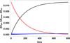 |
Fig. 9. Dimensionless variation of the waves and internal energies versus dimensionless time. Black: internal energy; red: Alfvén wave energy; blue: slow wave energy. (T = 12 000 K, v0 = 0.15, kz = π/2, ηC,0 = 0.0023). |
where EKA is the total kinetic energy of the Alfvén wave given by
where  the initial perturbation for the Alfvén wave. Therefore, the above expression provides us with the initial energy in the Alfvén wave. The Eint is the internal energy given by
where p(z) is the final pressure distribution and which, for the sake of simplicity, has been assumed as uniform and equal to p. Then, substituting the energy expressions in Eq. (93), we can obtain an expression for the final temperature, namely:
Then,
dividing by T0 and introducing cA,0, the temperature variation can be written in dimensionless form as
Using T0 = 12 000 K for the equilibrium temperature, ηC,0 = 0.045, and the equilibrium Alfvén and sound speeds, we obtain ΔT = 0.108. On the other hand, using the above-mentioned analytical solutions for pressure and density perturbations, Eq. (80), and the same physical conditions, we can compute the spatial average of temperature perturbation by means of
![$$ \begin{aligned} \langle T\prime [z,t]\rangle = \frac{1}{2 L}\int _{-L}^{L} T\prime [z,t] \ \mathrm{d}z .\end{aligned} $$](/articles/aa/full_html/2020/09/aa38220-20/aa38220-20-eq124.gif)
This computation is done for a time at which all the Alfvén wave’s energy has been converted to internal energy and the obtained result fully coincides with the value of ΔT that was obtained before.
3.2.2. Effect of radiation
In this case, our energy equation comes from Eq. (79), when thermal conduction is neglected and a radiative loss function (Hildner 1974) is considered. Then, the system of equations to be solved is:


![$$ \begin{aligned} \frac{\partial p\prime }{\partial t}&= - c_{\mathrm{s,0} }^2 \frac{\partial { v}_z\prime }{\partial z} + \left(\gamma -1 \right) \left[- \frac{c_{\mathrm{s,0} }^2}{\gamma } \left( \omega _\rho \ \rho \prime + \omega _T \left(\frac{\gamma }{c_{\mathrm{s,0} }^2}p\prime -\rho \prime \right) \right)\right]\nonumber \\&\quad +\left(\gamma -1 \right)\left[\eta _{\rm C,0}\left(\frac{\partial {B_{ y}\prime }}{\partial z}\right)^2 \right]\cdot \end{aligned} $$](/articles/aa/full_html/2020/09/aa38220-20/aa38220-20-eq127.gif)
This system was solved together with the same initial and boundary conditions as in Sect. 3.2.1. In order to determine the effect produced by radiative losses, we consider three different equilibrium temperatures, T = 12 000 K, T = 8000 K, and T = 6000 K, typical of quiescent solar prominences, together with two different values for L, 105 and 107 m, in an attempt to identify the effect of a change in the wavelength, λ = 4L, of the Alfvén wave. Next, the dimensionless numerical values of Cowling’s diffusity, ηC,0, are computed together with ωT and ωρ. Figures 10–11 show the temporal behavior of density, pressure, longitudinal velocity, and temperature perturbations for L = 105 m. The results show that for L = 105 m, the shorter wavelength, the perturbations corresponding to T = 12 000 K are quickly damped; for L = 107 m, the longer wavelength, the opposite happens and the perturbations corresponding to T = 6000 K are more quickly damped. This behavior can be understood following Soler (2010). In this work, the author obtained an analytical approximation for the imaginary part of the angular frequency, in the case of nonadiabatic slow waves in a filament thread. When radiation and thermal conduction are considered, the imaginary part of the angular frequency is given by
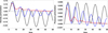 |
Fig. 10. Left panel: dimensionless density perturbations versus dimensionless time, with ambipolar diffusion and radiative losses included. Right panel: dimensionless pressure perturbations versus dimensionless time, with ambipolar diffusion and radiative losses included (z = 0, L = 105 m, T = 6000 K and ηC,0 = 0.03 (black curve), 8000 K and ηC,0 = 0.026 (blue curve), 12 000 K and ηC,0 = 0.023 (red curve)). |
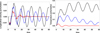 |
Fig. 11. Left panel: dimensionless longitudinal velocity perturbations versus dimensionless time, with ambipolar diffusion and radiative losses included computed at z = 0.5. Right panel: dimensionless temperature perturbations versus dimensionless time, with ambipolar diffusion and radiative losses included computed at z = 0 (L = 105 m, T = 6000 K and ηC,0 = 0.03 (black curve), 8000 K and ηC,0 = 0.026 (blue curve), 12 000 K and ηC,0 = 0.023 (red curve)). |
Then, once this quantity has been computed for the different temperatures, the damping time can be computed from

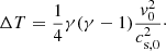
When only radiation is considered (κ∥ = 0), with the help of the Eqs. (103) and (104), we can obtain the damping times for each of the considered equilibrium temperatures and different values of L (see Table 2). For L = 107 m, the results show that the perturbations corresponding to the lower temperature are the ones that are more quickly damped. Conversely, when L is decreased to 105 m, the perturbations corresponding to the higher temperature are the ones that are more quickly damped. When only radiation is considered and the temperature is kept fixed, all the quantities in Eq. (103) are constants except the wavenumber, kz, which depends on L. Then, Eq. (104) can be written as
Damping times for slow waves.
suggesting a parabolic behavior of the damping time versus L, while F and G are constants. This can be seen in Fig. 12: for large values of L, no crosses between the different curves appear and the damping time is always much longer for high temperatures than for low ones. However, for small values of L, we observe the presence of crosses between the different curves and, as a consequence, the damping time for high temperatures is shorter than for low temperatures. For a constant temperature, the behavior of the damping time only depends on L (see Table 2), a quantity which is related to the longitudinal wavenumber through  .
.
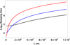 |
Fig. 12. Logarithm of the damping time versus L for T = 12 000 K (red), T = 8000 K (blue), T = 6000 K (black). |
On the other hand, for L = 105 m, the timescale is τ = 1.58 s, which means that the dimensionless time interval considered in Figs. 10 and 11 corresponds to 94.8 s. Then we can observe that: The perturbations are completely damped for a temperature of 12 000 K with a damping time of 49 s; they are slightly damped for 8000 K with a damping time of 104 s; and they are nearly undamped for 6000 K, with a damping time of 627 s. When L = 107 m is considered, the behavior of the temporal perturbation damping is reversed. The comparison between the obtained damping times (Table 2) and the temporal behavior of perturbations in Figs. 10 and 11 confirms that the analytical approximation is valid and explains the temporal attenuation of perturbations when different equilibrium temperatures, as well as different characteristic length scales, L, are considered.
Furthermore, it is also interesting to compare the damping times for Alfvén and slow waves. For L = 107 m, the damping times of Alfvén waves are much greater than those of slow waves, while the opposite happens when L = 105 m. Modifying the value of L means modifying the longitudinal wavenumber kz; therefore, when L is increased the wavenumber decreases and, following Eq. (68), the damping time is increased. Conversely, when L is decreased the damping time decreases. These results show that when the wavelength of the Alfvén wave, 4L, is increased, the efficiency of the ambipolar diffusion decreases and the opposite happens when is decreased. Then, when ambipolar diffusion is very efficient, Alfvén waves are quickly damped while slow waves still remain in the plasma; however, when ambipolar diffusion is inefficient, slow waves are more quickly damped. Figure 13 displays the temporal behavior of Alfvén, internal, and slow wave energies, showing how these energies are damped in time due to ambipolar and radiative losses. Then, taking into account the temporal behavior of the energies, we can explain the temporal behavior of the perturbations. At the beginning, they should behave as in the case without radiation; however, once radiative losses become dominant, these perturbations must be damped in time. Finally, Fig. 14 (left panel) shows the spatial distribution of the two terms contributing to the energy balance separately and for a fixed time; it can be seen that, for the chosen time, the injected heating is still dominant and radiative losses are small. Therefore, the balance is positive and the plasma is heated.
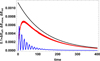 |
Fig. 13. Dimensionless variation of internal (red), slow (blue) and Alfvén (black) wave energies versus dimensionless time (T = 6000 K and ηC,0 = 0.003). |
3.2.3. Combined effect of radiation and thermal conduction
In this case, we must solve Eqs. (77)–(79) together with the following initial and boundary conditions:
Figure 14 (right panel) shows, at a fixed time, the spatial distribution of the balance between contributions coming from ambipolar diffusion, radiation, and thermal conduction; we observe that radiation dominates the energy loss while thermal conduction losses are negligible. This conclusion is in agreement with the temporal behavior of the different perturbations, which is quite similar to the case when only radiative losses are considered.
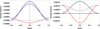 |
Fig. 14. Left panel: spatial distribution of the energy balance. Red curve: radiative losses; black curve: heating due to ambipolar diffusion; blue curve: radiative losses plus heating due to ambipolar diffusion (t = 1, T = 6000 K and ηC,0 = 0.003). Right panel: spatial distribution of the energy balance. Red curve: radiative losses; blue curve: thermal conduction losses; black curve: heating due to ambipolar diffusion; brown curve: radiative plus thermal conduction losses plus heating due to ambipolar diffusion (t = 3, T = 6000 K and ηC,0 = 0.0023). |
3.3. Third-order equations
The third-order equations represent nonlinear corrections to the Alfvén modes. The dimensionless third-order equations are:
These can be combined to obtain a wave equation for  so that
where f(z, t), the source term, is given by

This includes contributions coming from interactions between first-order magnetic-field and velocity perturbations with second-order longitudinal velocity and density perturbations. Eq. (109) was solved numerically with the following initial and boundary conditions:

In this case, we must take into account that second-order perturbations are influenced by thermal effects, which means that third-order magnetic-field and velocity perturbations for the Alfvén wave are also influenced by thermal effects. Figure 15 (left panel) shows the temporal behavior of third-order transverse velocity perturbation for the Alfvén wave when ambipolar diffusion and thermal effects are not taken into account. We can observe that the perturbation grows without bound due to the effect of the remaining source terms on the right-hand side of Eq. (109), as is consistent with the expected result that the nonlinearity of an ideal Alfvén wave increases with time. Conversely, Fig. 15 (right panel) compares the behavior of third-order velocity perturbation when thermal effects are or are not present in second-order perturbations. The main dissipative mechanism, producing the damping of third-order velocity perturbation, is Cowling’s difussivity; thermal effects, introduced by second-order perturbations, introduce an additional contribution to the damping of third-order Alfvénic perturbations. Thus, the presence of dissipative mechanisms reduces the nonlinearity of the Alfvén wave perturbations.
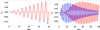 |
Fig. 15. Dimensionless third-order velocity perturbation computed at z = 0.5. Left panel: without ambipolar diffusion and second-order thermal effects. Right panel: (red) with ambipolar diffusion and without radiative and thermal conduction losses; (blue) with ambipolar diffusion and radiative losses (T = 12 000 K, ηC,0 = 0.023). |
On the other hand, as we state at the beginning of Sect. 3, contributions with higher orders in ϵ have been neglected. The inclusion of higher orders in ϵ would represent nonlinear corrections to the obtained Alfvén and slow waves, since fourth order in ϵ would involve  , p′, ρ′, and T′, again, while fifth-order in ϵ would represent higher corrections to Alfvén waves. However, because of the damping mechanisms, ambipolar diffusion, and thermal effects that are included in our calculations, the higher-order excited perturbations would probably have a negligible amplitude.
4. Nonlinear numerical simulations
4.1. Numerical method and setup
Now, we solve the nonlinear MHD equations numerically. The code used to perform the simulations is MoLMHD (Bona et al. 2009; Terradas et al. 2015, 2016, 2018). The full set of equations implemented in the code can be found in Terradas et al. (2015); they are reduced, without the nonideal terms, to Eqs. (36)–(40), which are shown in Sect. 2.4. The main features of the code are described in the following lines. The code is based on the method of lines technique and it solves the temporal and spatial parts independently. A third-order Runge-Kutta method is applied to the temporal part. Finite differences are used for the spatial part and a fifth-order WENO scheme (Jiang & Shu 1996) is applied for the velocity, density, and pressure variables. An ordinary fifth-order central scheme is used for the magnetic field, and no divergence correction is needed since the one-dimensional situation is considered; the full version of the code uses a hyperbolic correction based on Dedner et al. (2002). Although the comparison of MoLMHD to known standard shock MHD tests has not been published, the MoLMHD code shows the expected performance regarding the WENO implementation. The technique of background splitting for the magnetic field (see Powell et al. 1999) included in MoLMHD is not necessary in the present simulations. The novelty in this work is that the corresponding nonideal terms in the induction and pressure equation (Joule term) related to ambipolar diffusion need to be incorporated into the scheme. These terms are introduced in the code as source terms. The fact that we recover the linear results of the previous sections indicates that these source terms have been properly implemented in the code. For the present comparison, the rest of the nonideal terms, that is to say radiation, conduction, and heating terms, are not included in the equations. The time step, constrained by the CFL condition, is now also affected by the diffusion time due to ambipolar diffusion and it is modified accordingly. We use the same equilibrium in its simplest version, as we do in the previous sections. Therefore, we have constant density, pressure, and magnetic field pointing in the z-direction. For the initial perturbations (at t = 0) we focus on standing Alfvén waves around this equilibrium of the following form:
where v0 is the amplitude of the perturbation. Line-tying conditions are applied at the boundary of the domain and therefore no mass or energy is introduced in the system through the boundaries.
4.2. Results
First, we numerically tested the results for the linear regime. For comparison purposes, we plotted the density and temperature evolution obtained from the numerical solution of the nonlinear equations, and the solution using the regular perturbation approach presented earlier, in Fig. 16. The initial amplitude of excitation is v0 = 0.015, satisfying the condition of linearity. The agreement between the two solutions is remarkable, as can be seen when the two line styles are compared. This validates the numerical implementation in the code. Figure 16 indicates that in the strong diffusion situation, studied in the present simulations, we obtain the known effect already described in the linear regime; instead of an enhancement, there is a depletion around z = 0 and an enhancement at the footpoints, z = 1, a result that is essentially reversed in the absence of ambipolar diffusion.
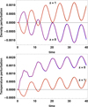 |
Fig. 16. Density (top panel) and temperature (bottom panel) as a function of time at two different positions (z = 0 and z = 1) in the linear regime (v0 = 0.015). The continuous line corresponds to the purely numerical results while the dashed line represents the semi-analytical approach developed in the previous sections. In this case, ηc = 0.045. |
Once we tested that the simulations agree with the known results and were confident that the numerical code works well, we carried out a brief nonlinear study. The results for a significantly larger initial amplitude of excitation, v0 = 0.3, are displayed in Fig. 17. In this case, the semi-analytical approach is no longer valid and the problem must be studied numerically. The results show the characteristic sawtooth profile in density and temperature that are associated with shocks. These shocks are due to the large-amplitude slow mode that is initially excited nonlinearly by the pump in the Alfvén wave. As we can see in the figure, they are not smoothed by the presence of ambipolar diffusion; only the Alfvénic component of the wave, not shown in the previous figures, is attenuated. We note how the periodicity in density and temperature fluctuations is reduced with respect to the linear case. Figure 17 also indicates that the overall increment in temperature in the system is significantly higher in this case when compared to the linear result of Fig. 16. The reason for this is that more energy is deposited in the Alfvén wave and therefore, due to ambipolar diffusion, this energy is transformed into heat that eventually raises the internal energy of the system. Even in this nonlinear situation, the analytical prediction of the temperature increment, given by Eq. (98), gives a value of 0.44, while the mean temperature increment from the simulations is 0.45. As mentioned in Sect. 1, Martínez-Gómez et al. (2018) used a multi-fluid approach to investigate the behavior of high-frequency nonlinear waves in a partially ionized plasma. For instance, when large initial amplitudes of the Alfvén waves were considered, the profiles of the second-order perturbations excited in a proton fluid look very similar to the profiles shown in Fig. 17.
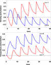 |
Fig. 17. Same as in Fig. 16, but for a large initial amplitude of excitation corresponding to the nonlinear regime (v0 = 0.3). |
Although the presence of shocks in the high-amplitude case is not described by the perturbation approach, the overall behavior of the wave perturbations is reasonably well described by the quasi-linear method, even when the Alfvén wave amplitude is a considerable fraction of the background Alfvén velocity.
5. Conclusions
We investigated the temporal behavior of nonlinear Alfvén waves considering a partially ionized plasma with prominence physical properties up to third order in the velocity amplitude when ambipolar diffusion is included as a dissipative mechanism for these waves. In the case of high amplitudes, linearly polarized Alfvén waves produce density perturbations and field-aligned motions, and self-interact with the induced perturbations. In our calculations, apart from ambipolar diffusion, we have also included radiative losses and thermal conduction as damping mechanisms for second-order perturbations. To develop this study, first, we considered a small-amplitude initial transverse velocity perturbation and applied the regular perturbations method. We obtained analytical solutions for the transverse velocity and magnetic field perturbations from first-order equations, as well as the period and damping time of the linear Alfvén waves. Next, we sought numerical solutions to the system of equations for second-order perturbations. We solved these equations with the aim of understanding the role played by ambipolar diffusion, radiative losses, and thermal conduction on second-order perturbations. When ambipolar diffusion is almost negligible, density perturbations at the center of the spatial domain are positive, while they are negative at the boundaries; the same happens for pressure and temperature perturbations because no heat is released at the center of the spatial domain. When ambipolar diffusion becomes important, we observe a depletion of density at the central part of the spatial domain and an enhancement at the boundaries. The reason for this behavior is the fact that the heat released due to ambipolar diffusion is deposited around the central part of the spatial domain and, as a consequence, the temperature rises, as does the pressure. In any case, the behavior of these perturbations can be understood from Eq. (80) and this behavior is strictly dependent on the strength of the ambipolar diffusion. Once we include radiative losses and thermal conduction in our calculations, second-order perturbations are damped in time and, using an analytical approximation for the imaginary part of the angular frequency in the non adiabatic case, the damping time can be estimated. Depending on the value of the characteristic scale length, L, this damping time is greater or smaller than the damping time for linear Alfvén waves. This indicates that after the excitation of second-order perturbations, Alfvén waves can be quickly damped while slow waves remain in the plasma, and vice versa. When dissipative mechanisms for slow waves are considered, the main damping mechanism for second-order perturbations is radiation, while the contribution of thermal conduction is very weak.
On the other hand, we computed the temporal behavior of the different energies involved in the process under investigation and the results show that almost all the initial energy in the Alfvén wave is transformed into plasma internal energy, producing an increment of temperature, while only a small amount is involved in the excitation of slow waves. This is interesting since this small amount of energy, which excites slow waves, allows for the continuous presence of these waves in the plasma in the absence of damping mechanisms for these waves. Also, making use of a simple approximation, we were able to compute the temperature increment, which shows an excellent agreement with the results from the numerical calculations. When dissipative mechanisms such as radiative losses and thermal conduction are included, the temporal behavior of the Alfvén energy shows how this energy is transferred to the plasma internal and slow wave energies which, later on, are also dissipated.
We also studied the effects induced by second-order perturbations and ambipolar diffusion on the nonlinear correction to the Alfvén waves described by third-order systems of equations. The results were compared to the case when ambipolar diffusion and thermal effects are neglected. In this case, the amplitude of the third-order transverse velocity perturbation grows without limit due to the effect of source terms; when ambipolar diffusion alone or ambipolar diffusion plus thermal effects are considered, the velocity perturbation is damped in time. The inclusion of thermal effects in second-order perturbations produces an additional contribution to the damping. Therefore, the contribution of dissipative effects causes the Alfvén wave to develop much smaller nonlinear corrections compared with the ideal Alfvén wave.
The case of large initial amplitudes of the Alfvén waves was studied by means of numerical simulations. First, we checked the semi-analytic results obtained in the linear regime and found a good agreement. Next, the fully nonlinear regime was explored by assuming a large initial amplitude; the profiles of the obtained perturbations show the sawtooth profile characteristic of associated shocks. Finally, the nonlinear results also show that the increment of plasma temperature can still be described by the linear approach.
As we summarized in Sect. 1, many authors have studied the damping of Alfvén waves in different contexts using analytical or numerical tools. For instance, nonlinear coupling of Alfvén waves exciting slow waves have mainly been studied in fully ionized plasmas (Hollweg 1971; Rankin et al. 1994; Tikhonchuk et al. 1995) and dissipative mechanisms such as resistivity or viscosity have sometimes been considered (Zheng et al. 2016). However, the nonlinear coupling of Alfvén and slow magnetoacoustic waves in partially ionized plasmas has received little attention. For instance, the nonlinear coupling of high-frequency standing and propagating Alfvén waves and slow waves was investigated by Martínez-Gómez et al. (2018) using a multi-fluid scheme. However, for our research, we used a different approach and focused our attention on the nonlinear coupling of Alfvén waves and slow waves in a partially ionized plasma that we considered to be a single fluid; additionally, we took dissipative mechanisms into account, such as ambipolar diffusion for Alfvén waves and thermal radiation and conduction for slow waves.
Finally, a potential application of this investigation relates to oscillations detected in partially ionized structures of the solar atmosphere, as was mentioned in Sect. 1, and solar prominences in particular. In many cases, the exciter of these oscillations is an energetic event, a flare, a jet, failed eruptions, Moreton waves, etc., which strongly perturb the equilibrium of the structure, injecting a large amount of energy and exciting large-amplitude oscillations. Then, longitudinal oscillations can be generated by nonlinear Alfvén waves that were initially excited, which can be quickly damped while slow waves remain for a longer time and are damped by radiative losses, as has been proposed in the case of filaments (Zhang et al. 2012, 2013), although other mechanisms such as mass accretion have also been proposed (Ruderman & Luna 2016). Therefore, in the full nonlinear case, when the amplitude of the initial Alfvénic perturbation is large, the amplitude of the generated longitudinal oscillations would be more important than in the weakly nonlinear case; these oscillations could represent small-amplitude oscillations reported in prominence observations (Arregui et al. 2018).
Acknowledgments
We acknowledge support from MINECO and FEDER funds through project AYA2017-85465-P. JLB and JT acknowledge discussions within the team on “Large-Amplitude Oscillations as a Probe of Quiescent and Erupting Solar Prominences”, led by M. Luna, and we all thank ISSI for their support. RS acknowledges the support from the “Ministerio de Economía, Industria y Competitividad” and the “Conselleria d’Innovació, Recerca i Turisme del Govern Balear (Pla de ciència, tecnologia, innovació i emprenedoria 2013–2017)” for the “Ramón y Cajal” grant RYC-2014-14970.
References
- Arregui, I., Oliver, R., & Ballester, J. L. 2018, Liv. Rev. Sol. Phys., 15, 3 [Google Scholar]
- Aschwanden, M. J. 2004, Physics of the Solar Corona. An Introduction [Google Scholar]
- Ballester, J. L. 2015, Solar Prominences, eds. J.-C. Vial, & O. Engvold, ASP Sci. Libr., 415, 259 [CrossRef] [Google Scholar]
- Ballester, J. L., Alexeev, I., Collados, M., et al. 2018, Space Sci. Rev., 214, 58 [NASA ADS] [CrossRef] [Google Scholar]
- Bona, C., Bona-Casas, C., & Terradas, J. 2009, J. Comput. Phys., 228, 2266 [CrossRef] [Google Scholar]
- Braginskii, S. I. 1965, Rev. Plasma Phys., 1, 205 [Google Scholar]
- Cally, P. S., & Khomenko, E. 2018, ApJ, 856, 20 [NASA ADS] [CrossRef] [Google Scholar]
- Cally, P. S., & Khomenko, E. 2019, ApJ, 885, 58 [CrossRef] [Google Scholar]
- Carbonell, M., Oliver, R., & Ballester, J. L. 2004, A&A, 415, 739 [NASA ADS] [CrossRef] [EDP Sciences] [Google Scholar]
- Cramer, N. F. 2001, The Physics of Alfvén Waves (Wiley-VCH) [Google Scholar]
- Dahlburg, R. B., & Mariska, J. T. 1988, Sol. Phys., 117, 51 [NASA ADS] [CrossRef] [Google Scholar]
- Dedner, A., Kemm, F., Kröner, D., et al. 2002, J. Comput. Phys., 175, 645 [Google Scholar]
- Erdélyi, R., & Goossens, M. 2011, Space Sci. Rev., 158, 167 [NASA ADS] [CrossRef] [Google Scholar]
- González-Morales, P. A., Khomenko, E., & Cally, P. S. 2019, ApJ, 870, 94 [CrossRef] [Google Scholar]
- Goossens, M. 2003, An Introduction to Plasma Astrophysics and Magnetohydrodynamics, 294 [CrossRef] [Google Scholar]
- Grant, S. D. T., Jess, D. B., Zaqarashvili, T. V., et al. 2018, Nat. Phys., 14, 480 [CrossRef] [Google Scholar]
- Heinzel, P., Vial, J. C., & Anzer, U. 2014, A&A, 564, A132 [NASA ADS] [CrossRef] [EDP Sciences] [Google Scholar]
- Heinzel, P., Gunár, S., & Anzer, U. 2015, A&A, 579, A16 [NASA ADS] [CrossRef] [EDP Sciences] [Google Scholar]
- Hildner, E. 1974, Sol. Phys., 35, 123 [NASA ADS] [CrossRef] [Google Scholar]
- Hollweg, J. V. 1971, J. Geophys. Res., 76, 5155 [NASA ADS] [CrossRef] [Google Scholar]
- Jess, D. B., Mathioudakis, M., Erdélyi, R., et al. 2009, Science, 323, 1582 [NASA ADS] [CrossRef] [PubMed] [Google Scholar]
- Jiang, G.-S., & Shu, C.-W. 1996, J. Comput. Phys., 126, 202 [NASA ADS] [CrossRef] [MathSciNet] [Google Scholar]
- Khomenko, E., & Cally, P. S. 2019, ApJ, 883, 179 [NASA ADS] [CrossRef] [Google Scholar]
- Klimchuk, J. A., & Cargill, P. J. 2001, ApJ, 553, 440 [NASA ADS] [CrossRef] [Google Scholar]
- Kohutova, P., Verwichte, E., & Froment, C. 2020, A&A, 633, L6 [NASA ADS] [CrossRef] [EDP Sciences] [Google Scholar]
- Landi, E., Del Zanna, G., Young, P. R., Dere, K. P., & Mason, H. E. 2012, ApJ, 744, 99 [NASA ADS] [CrossRef] [Google Scholar]
- Lardner, R. W., & Trehan, S. K. 1991, Ap&SS, 180, 93 [CrossRef] [Google Scholar]
- Lazarian, A. 2016, ApJ, 833, 131 [NASA ADS] [CrossRef] [Google Scholar]
- Leake, J. E., Arber, T. D., & Khodachenko, M. L. 2005, A&A, 442, 1091 [NASA ADS] [CrossRef] [EDP Sciences] [Google Scholar]
- Luna, M., Karpen, J., Ballester, J. L., et al. 2018, ApJS, 236, 35 [NASA ADS] [CrossRef] [Google Scholar]
- Martínez-Gómez, D., Soler, R., & Terradas, J. 2018, ApJ, 856, 16 [NASA ADS] [CrossRef] [Google Scholar]
- Mathioudakis, M., Jess, D. B., & Erdélyi, R. 2013, Space Sci. Rev., 175, 1 [NASA ADS] [CrossRef] [Google Scholar]
- Meier, E. T. 2011, Ph.D. Thesis, University of Washington, USA [Google Scholar]
- Milne, A. M., Priest, E. R., & Roberts, B. 1979, ApJ, 232, 304 [NASA ADS] [CrossRef] [Google Scholar]
- Nakariakov, V. M., & Verwichte, E. 2005, Liv. Rev. Sol. Phys., 2, 3 [Google Scholar]
- Nakariakov, V. M., Pilipenko, V., Heilig, B., et al. 2016, Space Sci. Rev., 200, 75 [NASA ADS] [CrossRef] [Google Scholar]
- Oliver, R. 1999, Magnetic Fields and Solar Processes, eds. A. Wilson, et al., ESA Spec. Publ., 9, 425 [Google Scholar]
- Oliver, R. 2009, Space Sci. Rev., 149, 175 [NASA ADS] [CrossRef] [Google Scholar]
- Powell, K. G., Roe, P. L., Linde, T. J., Gombosi, T. I., & De Zeeuw, D. L. 1999, J. Comput. Phys., 154, 284 [NASA ADS] [CrossRef] [Google Scholar]
- Priest, E. 2014, Magnetohydrodynamics of the Sun (Cambridge, UK: Cambridge University Press) [Google Scholar]
- Rankin, R., Frycz, P., Tikhonchuk, V. T., & Samson, J. C. 1994, J. Geophys. Res., 99, 21291 [NASA ADS] [CrossRef] [Google Scholar]
- Roberts, B. 2000, Sol. Phys., 193, 139 [NASA ADS] [CrossRef] [Google Scholar]
- Roberts, B. 2004, Oscillations and Small-Scale Transients Events in the Solar Atmosphere: Joint View from SOHO and TRACE, eds. H. Lacoste, ESA Spec. Publ., 547, 1 [Google Scholar]
- Roberts, B. 2006, Philos. Trans. R. Soc. London Ser. A, 364, 447 [NASA ADS] [CrossRef] [Google Scholar]
- Roberts, B. 2008, Waves & Oscillations in the Solar Atmosphere: Heating and Magneto-Seismology, R. Erdélyi, & C. A. Mendoza-Briceno, IAU Symp., 247, 3 [Google Scholar]
- Roberts, B., Edwin, P. M., & Benz, A. O. 1984, ApJ, 279, 857 [NASA ADS] [CrossRef] [Google Scholar]
- Rosner, R., Tucker, W. H., & Vaiana, G. S. 1978, ApJ, 220, 643 [NASA ADS] [CrossRef] [Google Scholar]
- Ruderman, M. S., & Luna, M. 2016, A&A, 591, A131 [NASA ADS] [CrossRef] [EDP Sciences] [Google Scholar]
- Soler, R. 2010, Ph.D. Thesis Departament de Fisica, Universitat de les Illes Balears, Spain [Google Scholar]
- Soler, R., Carbonell, M., & Ballester, J. L. 2015a, ApJ, 810, 146 [NASA ADS] [CrossRef] [Google Scholar]
- Soler, R., Ballester, J. L., & Zaqarashvili, T. V. 2015b, A&A, 573, A79 [NASA ADS] [CrossRef] [EDP Sciences] [Google Scholar]
- Soler, R., Terradas, J., Oliver, R., & Ballester, J. L. 2016, A&A, 592, A28 [NASA ADS] [CrossRef] [EDP Sciences] [Google Scholar]
- Song, P., Vasyliūnas, V. M. 2011, J. Geophys. Res. Space, 116 [Google Scholar]
- Spitzer, L. 1962, Physics of Fully Ionized Gases (New York: Interscience) [Google Scholar]
- Srivastava, A. K., Shetye, J., Murawski, K., et al. 2017, Sci. Rep., 7, 43147 [NASA ADS] [CrossRef] [Google Scholar]
- Terradas, J., & Ofman, L. 2004, ApJ, 610, 523 [NASA ADS] [CrossRef] [Google Scholar]
- Terradas, J., Soler, R., Luna, M., Oliver, R., & Ballester, J. L. 2015, ApJ, 799, 94 [NASA ADS] [CrossRef] [Google Scholar]
- Terradas, J., Soler, R., Luna, M., et al. 2016, ApJ, 820, 125 [NASA ADS] [CrossRef] [Google Scholar]
- Terradas, J., Magyar, N., & Van Doorsselaere, T. 2018, ApJ, 853, 35 [NASA ADS] [CrossRef] [Google Scholar]
- Threlfall, J., McClements, K. G., & De Moortel, I. 2011, A&A, 525, A155 [NASA ADS] [CrossRef] [EDP Sciences] [Google Scholar]
- Thurgood, J. O., & McLaughlin, J. A. 2013, Sol. Phys., 288, 205 [NASA ADS] [CrossRef] [Google Scholar]
- Tikhonchuk, V. T., Rankin, R., Frycz, P., & Samson, J. C. 1995, Phys. Plasmas, 2, 501 [NASA ADS] [CrossRef] [Google Scholar]
- Tomczyk, S., McIntosh, S. W., Keil, S. L., et al. 2007, Science, 317, 1192 [NASA ADS] [CrossRef] [PubMed] [Google Scholar]
- Vernazza, J. E., Avrett, E. H., & Loeser, R. 1981, ApJS, 45, 635 [Google Scholar]
- Verwichte, E., Nakariakov, V. M., & Longbottom, A. W. 1999, J. Plasma Phys., 62, 219 [NASA ADS] [CrossRef] [Google Scholar]
- Vranjes, J., & Krstic, P. S. 2013, A&A, 554, A22 [NASA ADS] [CrossRef] [EDP Sciences] [Google Scholar]
- Zaqarashvili, T. V., Carbonell, M., Ballester, J. L., & Khodachenko, M. L. 2012, A&A, 544, A143 [NASA ADS] [CrossRef] [EDP Sciences] [Google Scholar]
- Zaqarashvili, T. V., Khodachenko, M. L., & Soler, R. 2013, A&A, 549, A113 [NASA ADS] [CrossRef] [EDP Sciences] [Google Scholar]
- Zhang, Q. M., Chen, P. F., Xia, C., & Keppens, R. 2012, A&A, 542, A52 [NASA ADS] [CrossRef] [EDP Sciences] [Google Scholar]
- Zhang, Q. M., Chen, P. F., Xia, C., Keppens, R., & Ji, H. S. 2013, A&A, 554, A124 [NASA ADS] [CrossRef] [EDP Sciences] [Google Scholar]
- Zheng, J., Chen, Y., & Yu, M. Y. 2016, Phys. Scr., 91, 035601 [CrossRef] [Google Scholar]
Appendix A: Coefficients of the polynomial fit
The numerical values of the coefficients of the polynomial fit (Eq. (9)) are:
All Tables
Numerical values of the piecewise constants χ* and α for prominences (Hildner 1974).
All Figures
|
Fig. 1. Ionization degree i versus temperature T and pressure p. The blue dots correspond to data in Table 1 in Heinzel et al. (2015); the surface represents the fitting described by Eq. (9). |
| In the text | |
|
Fig. 2. Dimensionless linear Alfvén wave velocity (red) and magnetic field perturbations (blue) versus dimensionless time. The velocity amplitude has been computed at z = 0, while the magnetic field amplitude has been computed at z = 1 (T = 12 000, v0 = 0.15, kz = π/2, ηC,0 = 0.0023). |
| In the text | |
|
Fig. 3. Dimensionless heating versus dimensionless time and space for ηC,0 = 0.023. |
| In the text | |
|
Fig. 4. Dimensionless pressure perturbations versus dimensionless time computed at z = 0 (left) and z = 1 (right), for ηC,0 = 0.00023 (black), 0.023 (blue), and 0.045 (red). |
| In the text | |
|
Fig. 5. Dimensionless density perturbations versus dimensionless time computed at z = 0 (left) and z = 1 (right), for ηC,0 = 0.00023 (black), 0.023 (blue), and 0.045 (red). |
| In the text | |
|
Fig. 6. Dimensionless temperature perturbations versus dimensionless time computed at z = 0 (left) and z = 1 (right), for ηC,0 = 0.00023 (black), 0.023 (blue), and 0.045 (red). |
| In the text | |
|
Fig. 7. Left panel: dimensionless longitudinal velocity perturbations versus dimensionless time computed for ηC,0 = 0.00023 (black), 0.023 (blue), and 0.045 (red); Right panel: dimensionless longitudinal velocity perturbation versus dimensionless time. Full analytical solution obtained from Eq. (89) (red) and numerical solution (blue) (z = 0.5, v0 = 0.15, kz = π/2, ηC,0 = 0.045 and 0.00023). |
| In the text | |
|
Fig. 8. Dimensionless density perturbation versus dimensionless time and space for ηC,0 = 0.045. |
| In the text | |
|
Fig. 9. Dimensionless variation of the waves and internal energies versus dimensionless time. Black: internal energy; red: Alfvén wave energy; blue: slow wave energy. (T = 12 000 K, v0 = 0.15, kz = π/2, ηC,0 = 0.0023). |
| In the text | |
|
Fig. 10. Left panel: dimensionless density perturbations versus dimensionless time, with ambipolar diffusion and radiative losses included. Right panel: dimensionless pressure perturbations versus dimensionless time, with ambipolar diffusion and radiative losses included (z = 0, L = 105 m, T = 6000 K and ηC,0 = 0.03 (black curve), 8000 K and ηC,0 = 0.026 (blue curve), 12 000 K and ηC,0 = 0.023 (red curve)). |
| In the text | |
|
Fig. 11. Left panel: dimensionless longitudinal velocity perturbations versus dimensionless time, with ambipolar diffusion and radiative losses included computed at z = 0.5. Right panel: dimensionless temperature perturbations versus dimensionless time, with ambipolar diffusion and radiative losses included computed at z = 0 (L = 105 m, T = 6000 K and ηC,0 = 0.03 (black curve), 8000 K and ηC,0 = 0.026 (blue curve), 12 000 K and ηC,0 = 0.023 (red curve)). |
| In the text | |
|
Fig. 12. Logarithm of the damping time versus L for T = 12 000 K (red), T = 8000 K (blue), T = 6000 K (black). |
| In the text | |
|
Fig. 13. Dimensionless variation of internal (red), slow (blue) and Alfvén (black) wave energies versus dimensionless time (T = 6000 K and ηC,0 = 0.003). |
| In the text | |
|
Fig. 14. Left panel: spatial distribution of the energy balance. Red curve: radiative losses; black curve: heating due to ambipolar diffusion; blue curve: radiative losses plus heating due to ambipolar diffusion (t = 1, T = 6000 K and ηC,0 = 0.003). Right panel: spatial distribution of the energy balance. Red curve: radiative losses; blue curve: thermal conduction losses; black curve: heating due to ambipolar diffusion; brown curve: radiative plus thermal conduction losses plus heating due to ambipolar diffusion (t = 3, T = 6000 K and ηC,0 = 0.0023). |
| In the text | |
|
Fig. 15. Dimensionless third-order velocity perturbation computed at z = 0.5. Left panel: without ambipolar diffusion and second-order thermal effects. Right panel: (red) with ambipolar diffusion and without radiative and thermal conduction losses; (blue) with ambipolar diffusion and radiative losses (T = 12 000 K, ηC,0 = 0.023). |
| In the text | |
|
Fig. 16. Density (top panel) and temperature (bottom panel) as a function of time at two different positions (z = 0 and z = 1) in the linear regime (v0 = 0.015). The continuous line corresponds to the purely numerical results while the dashed line represents the semi-analytical approach developed in the previous sections. In this case, ηc = 0.045. |
| In the text | |
|
Fig. 17. Same as in Fig. 16, but for a large initial amplitude of excitation corresponding to the nonlinear regime (v0 = 0.3). |
| In the text | |
Current usage metrics show cumulative count of Article Views (full-text article views including HTML views, PDF and ePub downloads, according to the available data) and Abstracts Views on Vision4Press platform.
Data correspond to usage on the plateform after 2015. The current usage metrics is available 48-96 hours after online publication and is updated daily on week days.
Initial download of the metrics may take a while.