© A. Prabhu et al. 2020

1. Introduction

Astrophysical bodies such as stars, galaxies, and planets are known to posses magnetic fields, typically on scales as large as those systems themselves. Dynamo theory aims to describe the mechanisms responsible for the generation and maintenance of these magnetic fields from first principles. Specifically, the solar magnetic field and its spatio-temporal features (such as the cyclic polarity reversals) are ascribed to a dynamo process acting within the Sun’s convection zone. One scenario attempts to explain the origin of solar magnetism with the α effect (Moffatt 1978; Krause & Rädler 1980; Brandenburg et al. 2012). In this framework, kinetic helicity (a measure of handedness) of the gas motions, is believed to play a central role in the generation of large-scale magnetic fields in the Sun. This also results in the production of magnetic helicity, which can be interpreted in terms of twist of flux tubes or linkage of magnetic field lines (Berger & Field 1984; Blackman 2015). The volume integral of the magnetic helicity density is almost perfectly conserved – even in non-ideal magnetohydrodynamics (MHD); see Berger (1984). This imposes important constraints on the evolution of magnetic fields via a dynamo mechanism (Brandenburg & Subramanian 2005). For the solar dynamo, the combined effect of stratification and global rotation are believed to be responsible for the α effect (Krause & Rädler 1980). The α effect encapsulates the helical nature of turbulence within the solar convection zone. A key consequence of the α effect is the presence of opposite signs of magnetic helicity at small and large scales (Seehafer 1996). Such magnetic fields are now referred to as bihelical (Yousef & Brandenburg 2003) or doubly helical (Blackman & Brandenburg 2003). Additionally, due to the reflectional antisymmetry of cyclonic convection across the equator, α changes sign at the equator (Parker 1955). Consequently, the magnetic helicity not only has opposite signs at large and small scales, but it also changes sign across the equator. Thus, from theoretical considerations we expect a hemispheric sign rule for magnetic helicity in the Sun. Specifically, one expects a positive (negative) sign of magnetic helicity at large (small) scales in the Northern hemisphere and vice versa in the Southern hemisphere. Here, a small-scale field is defined as the difference between actual and averaged fields. In that sense, even the scale of active regions (ARs) must be regarded as ‘small’ because the large-scale field as seen in the solar butterfly diagram, is obtained through azimuthal averaging, which also washes out ARs.

Much effort has been devoted to characterising the behaviour of magnetic helicity in the Sun. The primary motivation is to test the predictions of the α effect and thus indirectly verify the significance of the α effect for the solar dynamo. The earliest efforts were those of Seehafer (1990) and Pevtsov et al. (1995), who analysed the magnetic field in local Cartesian patches and used the vertical or z component of the current helicity ⟨j_zb_z⟩ as a proxy for magnetic helicity. Here j ∝ ∇ × b is the current density and b is the magnetic field. These studies focused on the helicity associated with ARs, and they found it to be mostly positive (negative) in the Southern (Northern) hemisphere. However, given the aforementioned dependence of helicity on the scale, a more complete picture can be obtained by looking at the spectra of magnetic helicity (Zhang et al. 2014, 2016). A more global approach, taking into account the change in sign of helicity across the equator was developed by Brandenburg et al. (2017), called the two-scale approach after Roberts & Soward (1975). This was followed by a systematic study employing this two-scale approach over a large sample of Carrington rotations from solar cycle 24 by Singh et al. (2018). They provided evidence for the expected hemispheric sign rule in the Sun, specifically during the rising phase of cycle 24.

All the studies mentioned so far rely on the determination of the magnetic field on the Sun’s photosphere. This is usually done by measuring the full Stokes vector, (I, Q, U, V), where I is the intensity, Q and U are the components of linear polarisation, and V is circular polarisation. Typically, for the retrieval of the magnetic field at the photosphere, the Zeeman effect is used as a diagnostic. One attempts to deduce an atmospheric stratification that best fits the spectropolarimetric observations (del Toro Iniesta & Ruiz Cobo 2016). Thus, the magnetic field vector is not a direct measurement but rather an inference. In addition, the use of Zeeman diagnostics bears an intrinsic ambiguity, referred to as the π ambiguity, associated with the transverse (perpendicular to the line-of-sight) component of the magnetic field. That is, we can only see it as an arrow-less vector in the line-of-sight coordinate system. For the conversion to a solar coordinate system, several disambiguation methods exist, based on potential field extrapolations or on minimum energy techniques; see Metcalf et al. (2006) for a review. However, these methods have limitations and fail to work accurately in complex magnetic field topologies or where the determination of the field is strongly influenced by the noise in the measurement. The errors introduced by these disambiguation methods can have a drastic impact on the computation of magnetic helicity. Hence, a means of inferring the helicity of magnetic fields, independent of the π ambiguity, is desired.

Brandenburg et al. (2019) introduced a possible proxy for helical magnetic fields, which could circumvent the uncertainty introduced by the π ambiguity. They used Stokes Q and U polarisation measurements, and decomposed them into rotationally invariant E and B polarisations (Kamionkowski et al. 1997; Seljak & Zaldarriaga 1997; Durrer 2008). The E and B polarisations are parity-even and parity-odd quantities, respectively. Correlations of B polarisation with parity-even quantities such as E polarisation or temperature T can be indicative of the helicity of the underlying magnetic field (Pogosian et al. 2002; Kahniashvili & Ratra 2005; Kahniashvili et al. 2014). We expect that the sign of magnetic helicity changes across the equator at both large and small length scales. Thus, we expect the EB correlation to reflect this behaviour and have systematically different signs in the two hemispheres. Brandenburg et al. (2019) used this EB decomposition and tested it with full disk polarisation data from the Vector SpectroMagnetograph (VSM) instrument of the Synoptic Optical Long-term Investigations of the Sun (SOLIS) project. However, they did not find significant non-zero parity-odd correlations from their analysis. Brandenburg (2019) extended this work to a fully global approach using spin-weighted spherical harmonics. He focussed on the calculation of a global spectrum of the EB correlation by taking into account its systematic sign change across the equator. Local aspects and features of the E and B patterns were completely ignored, however.

For the present analysis, we adopt the local approach and focus on linear polarisation measurements of ARs from both hemispheres. We use the polarisation measurements obtained by the Solar Dynamics Observatory (SDO). We then decompose this linear polarisation into E and B polarisations. The aim of this study is to test if there are significant non-vanishing EB correlations from solar ARs and if they show a systematic preference of a sign based on hemisphere. Therefore, we look at a sample of ARs and analyse the EB correlations and patterns computed from them in detail. However, there are a few drawbacks of using polarisation data as is. They may have some systematic instrumental effects that need to be accounted for. Additionally, there are Doppler shifts of spectral lines and magneto-optical effects which also leave their imprint on the measured spectropolarimetric observations. Due to Faraday rotation, which is one of two magneto-optical effects, a constant non-helical magnetic field can give rise to a non-zero EB correlation. This property was utilised in theoretical studies of the cosmic microwave background radiation (Kosowsky & Loeb 1996; Scannapieco & Ferreira 1997; Scóccola et al. 2004). However, for the purpose of this study, it is necessary to disentangle the contributions of the intrinsic helicity of magnetic fields from those of Faraday rotation, because both can cause a non-zero EB correlation.

In Sect. 2, we briefly review the motivations for the EB decomposition and its relation to linear polarisation. In Sect. 3, we discuss the observations and define correlation spectra that we determine from those observations. We also address the influence of Faraday rotation on our conclusions. We conclude with a discussion and interpretation of our results in Sect. 4.

2. E and B polarisations

We begin by recalling some basics of polarised radiative transfer. Let I(τ_c)=(I, Q, U, V)^T be the Stokes vector for which the radiative transfer equation (RTE) can be written as

$$\begin{array}{c}\hfill \frac{\mathrm{d}\mathit{I}}{\mathrm{d}{\tau }_c}=\mathit{K}(\mathit{I}-\mathit{S}).\end{array}$$(1)

Here τ_c is the optical depth at the continuum wavelength, and K is the propagation matrix, wherein the diagonal terms correspond to absorption, and the off-diagonal terms are responsible for dichroism and dispersion. The latter exchanges the states of polarisation caused by phase shifts during the propagation, which includes the following two magneto-optical effects: the exchange between the linear polarised components (Q and U) is called Faraday rotation, and between linear and circular polarised components (Q, U and V) Faraday pulsation. S is the source-function vector, which, under the assumption of local thermodynamic equilibrium (LTE), can be approximated as S ≡ (B_ν(T),0, 0, 0), where B_ν(T) is the Planck function. The measured quantity is I(τ_c = 0), and it is given by the formal solution of the RTE (Landi Degl’Innocenti & Landi Degl’Innocenti 1985). The observable complex linear polarisation, P(x, y) = Q + iU, can be decomposed into the rotationally invariant parity-even and parity-odd E and B polarisations, respectively. Here, x and y are local Cartesian coordinates on the solar disk. We thus invoke the small-scale limit, that is, we focus on small patches on a sphere, where the curvature can be neglected. The amplitudes of Stokes Q and U depend on the orientation of the polarisation basis. It is thus desirable to transform this linear polarisation into quantities which are rotationally invariant that is, E and B. As mentioned before, E and B behave differently under parity transformation; E remains unchanged whereas B changes sign. This is analogous to the directionality of electric and magnetic fields, which are proper and pseudo vectors, respectively.

Following Brandenburg et al. (2019), we define R = E + iB. We discuss the details of the E and B decomposition from linear polarisation in the small-scale limit and the two sign conventions in Appendix A. The sign convention adopted here agrees with that of Brandenburg et al. (2019), but is different from the one in Brandenburg (2019), who followed the convention of Durrer (2008). In the small-scale limit, R is related to P in Fourier space (indicated by tildes) via the following relation (for details, see Zaldarriaga & Seljak 1997; Seljak 1997)

$$\begin{array}{c}\hfill \stackrel{\sim }{R}(k_x,k_y)={({\widehat{k}}_x-i{\widehat{k}}_y)}^2\stackrel{\sim }{P}(k_x,k_y),\end{array}$$(2)

where ${\widehat{k}}_x$ and ${\widehat{k}}_y$ are x and y components (in the plane of the image) of the unit vector $\widehat{\mathit{k}}=\mathit{k}/k$, where k = |k| is the length of k = (k_x, k_y). Upon transformation of $\stackrel{\sim }{R}$ back to real space, we have maps of E(x, y) and B(x, y) corresponding to a set of Q and U maps at a certain wavelength. It is useful to compute shell-integrated spectra in wavenumber space for a given radius k as

$$\begin{array}{c}\hfill C_{\mathit{XY}}^i(k)={\displaystyle {\int }_0^{2\pi }{\tilde{X}}_i(\mathit{k}){\tilde{Y}}_i^{\ast }(\mathit{k})k\mathrm{d}{\varphi }_k,}\end{array}$$(3)

where the asterisk denotes complex conjugation, ${\stackrel{\sim }{X}}_i$ and ${\stackrel{\sim }{Y}}_i$ stand for ${\stackrel{\sim }{E}}_i$, ${\stackrel{\sim }{B}}_i$, or $\stackrel{\sim }{T}$ (T represents temperature), and i characterises the wavelength bin at which we compute E and B. For T we take the continuum intensity as a proxy, so there is no subscript i. Finally, we also define the normalised antisymmetric spectra as

$$\begin{array}{c}\hfill c_{\mathrm{A}}^{\mathit{XY}}(k)=\frac{{\sum }_{i}2C_{\mathit{XY}}^i(k)}{{\sum }_i[C_{\mathit{XX}}^i(k)+C_{\mathit{YY}}^i(k)]},\end{array}$$(4)

which we use throughout our analysis; see Appendix B for examples.

We considered between four and six wavelength bins, as is explained in more detail in Sect. 3.1. However, in some cases (Sect. 3.5), we inferred Stokes Q and U from the components of the transverse magnetic field, in which case there is no wavelength dependence.

3. Application to solar observations

3.1. Observations used in this study

In this section, we briefly describe the solar observations from the Helioseismic and Magnetic Imager (HMI, Schou et al. 2012), on board SDO, used in this analysis. We used the publicly available polarisation measurements and magnetic field vector data at different stages in our analysis. For the polarisation measurements, we used level-1 reduced data. Here we only focus on Stokes Q and U; Stokes I and V are not included in our study. SDO/HMI provides full disk images of Stokes Q and U which were cropped to the relevant ARs. The magnetic field vector data are the result of the VFISV inversion code (Borrero et al. 2011), and a disambiguation based on the minimum energy method (Metcalf 1994; Leka et al. 2009). We used the SHARP data product (Bobra et al. 2014) from the HMI team, which provides the definitive b = (b_r, b_θ, b_ϕ) which has been remapped to a Lambert Cylindrical Equal-Area projection and decomposed into b_r, b_θ, and b_ϕ. These however are not full disk, but partial-disk patches, automatically identified and cropped around the ARs.

We chose a small, random sample of ARs from solar cycle 24 (see Table 1). We examined the antisymmetric polarisation correlations (see Sect. 2), c_A, calculated from Stokes Q and U measurements of the ARs. To reiterate, the aim is to check whether we see a systematic preference for the sign of c_A based on hemisphere, thus reflecting the hemispheric sign rule for magnetic helicity.

HMI is a filtergraph which samples the 6173Å Fe I absorption line at 6 positions in wavelength with a spacing of 69 mÅ. The full width half maximum of the filter at each of these wavelengths is 76 mÅ ± 10 mÅ, we therefore refer to them as wavelength bins λ_i, where i = 0–5. Here λ₀ is the extreme blue position of the filter, and λ₅ is the extreme red position.

We produced maps of Stokes Q and U at all wavelength bins within the 6173Å Fe I line, on both the blue and red wings. From the Stokes maps we then computed the E and B polarisations using Eq. (2) and also the shell-integrated spectra, Eq. (3), at these wavelength bins. As mentioned before, Faraday rotation can possibly contribute to a non-zero EB correlation, even in the absence of magnetic helicity. Its effects are strongest near or at the line core, depending on the strength of the magnetic field. We studied these ARs on the central meridian, so the Doppler shifts due to solar rotation and Evershed flow are minimised. However, there are also Doppler shifts due to the orbital velocity of SDO, resulting in the line core being sampled by λ₂ or λ₃. We note that in extreme cases these shifts due to the orbital velocity could be large enough for the line core to be sampled by λ₁ or λ₄. For these reasons, we obtain c_A from the averaged E and B spectra computed at λ₀, λ₁, λ₄, λ₅ and analyse the EB correlation from λ₂ and λ₃ separately (Sect. 3.6).

We separated the 18 ARs of Table 1 into three categories based on the sign of the EB correlation $c_{\mathrm{A}}^{\mathit{EB}}(k)$. Category A (12 ARs) is for ARs whose normalised $c_{\mathrm{A}}^{\mathit{EB}}(k)$ spectra show a preference for a particular sign that is in agreement with the expected hemispheric sign rule for magnetic helicity (see Sect. 1). Category B (3 ARs) is for ARs that show the opposite sign for $c_{\mathrm{A}}^{\mathit{EB}}(k)$ than what is expected from theoretical considerations. Finally, category C (3 ARs) is for ARs that do not show any clear preference for the sign of $c_{\mathrm{A}}^{\mathit{EB}}(k)$. The dataset containing the shell-integrated spectra defined in Eq. (3), along with maps of E and B for each AR can be found in an online catalogue¹.

3.2. ARs from category A

Firstly, we present in Fig. 1 (first column) the spectra $c_{\mathrm{A}}^{\mathit{EB}}(k)$ of correlations of E and B calculated from Stokes Q and U at four wavelengths (λ₀, λ₁, λ₄, λ₅); see Eq. (4). In our analysis, we find that the ARs from the Northern (Southern) hemisphere, have a preference for a negative (positive) sign of $c_{\mathrm{A}}^{\mathit{EB}}$. The non-zero $c_{\mathrm{A}}^{\mathit{EB}}$ correlations computed from those wavelength bins where the influence of Faraday rotation should be negligible, suggest that these correlations are indeed a proxy for helical magnetic fields.

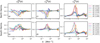Fig. 1. $c_{\mathrm{A}}^{\mathit{EB}}(k)$, $c_{\mathrm{A}}^{\mathit{TB}}(k)$, and $c_{\mathrm{A}}^{\mathit{TE}}(k)$ (first, second, and third column) for the ARs of category A from the Northern hemisphere (top row) and Southern hemisphere (bottom row) (see Table 1), using Eq. (4) with E and B being computed at λ0, λ1, λ4, λ5.

As discussed in Sect. 1, helical magnetic fields can contribute to parity-odd correlations. In addition to correlations between E and B, there can also be parity-odd correlation from T and B ($c_{\mathrm{A}}^{\mathit{TB}}$), temperature being a parity-even quantity. We used the continuum intensity, which is an excellent proxy for the temperature of the photosphere. Figure 1 (middle column) shows the resulting spectra, which are an average of four wavelength bins (λ₀, λ₁, λ₄, λ₅). In accordance with $c_{\mathrm{A}}^{\mathit{EB}}$, one observes a hemispheric sign preference for $c_{\mathrm{A}}^{\mathit{TB}}$ correlations: negative (positive) in the Northern (Southern) hemisphere. The non-zero values of $c_{\mathrm{A}}^{\mathit{TB}}$ along with the systematic preference for the sign is yet another indicator that these antisymmetric correlations are a result of helical fields. This sign preference is especially prominent for scales between 1 and 10 Mm.

By studying the analogously computed correlations of T and E ($c_{\mathrm{A}}^{\mathit{TE}}$), we can have another confirmation that it is indeed B that is changing sign with hemisphere and not E. The $c_{\mathrm{A}}^{\mathit{TE}}$ correlations (Fig. 1, third column) mostly maintain the same positive sign for ARs from both hemispheres, which is expected given the parity-even nature of E (see Appendix A).

3.3. ARs from category B

Out of the ARs that we looked at in this study, we also found ARs that show an opposite sign of $c_{\mathrm{A}}^{\mathit{EB}}$ than what is expected from the hemispheric sign rule (Fig. 2, solid lines). We expect the sign for an AR in the North (South) to have a negative (positive) sign of magnetic helicity. ARs 11543 (North) and 12415, 12194 (South) show opposite signs, positive and negative, respectively. This is not surprising as such, since in most statistical studies that look at helicity of isolated patches of ARs, there is always a certain percentage of ARs that do not conform to the hemispheric sign rule for helicity (Pevtsov et al. 1995; Singh et al. 2018; Gosain & Brandenburg 2019). The latitude or the complexity class of the ARs does not seem to play a role in the reversed sign of the EB correlations, as ARs of a similar latitude or complexity also belong to category A.

Fig. 2. Similar to Fig. 1, but the ARs of categories B (solid lines) and C (dashed lines).

For the category B cases, analogously to the category A cases, we also looked at correlations between T and B, $c_{\mathrm{A}}^{\mathit{TB}}(k)$, and also between T and E, $c_{\mathrm{A}}^{\mathit{TE}}(k)$. First, looking at $c_{\mathrm{A}}^{\mathit{TB}}(k)$ (Fig. 2, second column), AR 11543 displays a distinctly bimodal behaviour in that there are positive and negative values of $c_{\mathrm{A}}^{\mathit{TB}}(k)$ at slightly different values of k. This is in contrast to ARs of category A, where the TB correlations showed a clear preference for a particular sign, in accordance with the sign of EB correlations. By contrast, for ARs 12415 and 12194, the EB and TB correlations have the same negative sign. As previously, the TE correlations (Fig. 2, third column) are positive for both hemispheres and in the case of AR 11543, $c_{\mathrm{A}}^{\mathit{TE}}(k)$ shows an unusual double-peaked spectrum.

3.4. ARs from category C

The third category is for ARs that do not show a clear preference for a sign (Fig. 2, dashed lines) of $c_{\mathrm{A}}^{\mathit{EB}}$. Looking at TB correlations for this category, the two ARs from the Northern hemisphere display almost no signal. However, the TB correlations for the Southern AR 11494 show a bimodal behaviour, similar to AR 11543 from category B. A similar hemispheric distinction can also be seen for the TE correlations, where for the Northern ARs there is almost no signal, and for the Southern AR we have a clear positive sign.

3.5. EB correlations computed from the magnetic field

Until now, we have decomposed the measured Stokes Q and U into E and B polarisations. Here, following Brandenburg (2019), we made an attempt to compute E and B (thus also $c_{\mathrm{A}}^{\mathit{EB}}$) from the magnetic field data. This is because the components of the magnetic field vector, used to compute c_A, are from a spectropolarimetric inversion wherein the magneto-optic effects and Doppler shifts are accounted for. If we observe a region closer to the center of the solar disk, we can, to a certain degree, assume that

$$\begin{array}{c}\hfill P\equiv Q+iU=-ϵ{(b_{\theta }+i{b}_{\varphi })}^2,\end{array}$$(5)

where ϵ in the present context is a proportionality constant that depends on the heliocentric angle and b_θ, b_ϕ are the transverse field components in the medium. Equation (5) is an approximation of the otherwise complex relation between Stokes Q and U to the transverse components b_θ, b_ϕ. There are two things that we must note here. Firstly, we are assuming that the Stokes Q and U signals are only due to the magnetic field components parallel to the solar surface (transverse components). However, this is valid only at low heliocentric angles; farther away from the disk center the validity of this assumption is poor. Secondly, as pointed out in Brandenburg (2019), the π ambiguity associated with the transverse components (b_θ, b_ϕ) does not affect this assumption, that is, a flip of 180° of the transverse component does not change the sign of P. When we compute the $c_{\mathrm{A}}^{\mathit{EB}}$ from the magnetic field, we do this from maps of b_θ and b_ϕ by exploiting Eq. (5). In the following, since we are only interested in normalised quantities such as c_A(k), which are relative measurements, we put ϵ = 1.

We show in Fig. 3 the spectrum $c_{\mathrm{A}}^{\mathit{EB}}$ computed from b_θ and b_ϕ for all ARs. First we look at ARs of category A (Fig. 3, left column). The preference for a negative (positive) sign of c_A in the Northern (Southern) hemispheres is evident, although it is definitely less clear than when $c_{\mathrm{A}}^{\mathit{EB}}$ is computed directly from linear polarisation (Fig. 1, first column). This is especially true of the case of AR 11546, which would be classified as an AR of category B, if one looks at $c_{\mathrm{A}}^{\mathit{EB}}$ computed from the magnetic field (see left panel of Fig. 3) with the simplifying assumption mentioned in the paragraph above. This weaker preference can be attributed to the imperfect validity of Eq. (5) at AR latitudes further away from the equator, since the linear polarisation in this case has a significant additional contributions from b_r. For category B (Fig. 3, right column, solid lines), the preference for the reversed sign of EB correlations is also quite discernible. And lastly, for category C, even for the EB correlations computed using Eq. (5), an obvious preference for either of the signs is absent. However, regardless of the categories, one can notice good agreement in the shape of the spectra of individual ARs computed from the magnetic field (Fig. 3) and those computed from Stokes Q and U (Figs. 1 and 2, first column). This agreement between the spectra is an indication that the c_A correlations we see from Stokes Q and U are indeed indicative of the intrinsic magnetic helicity of the ARs, and not a result of Faraday rotation from a non-helical magnetic field.

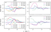Fig. 3. $c_{\mathrm{A}}^{\mathit{EB}}(k)$ for ARs of categories A (left column), B (right column, solid lines), and C (right column, dashed lines), with E and B being calculated from the components of the magnetic field vector. The curves for $c_{\mathrm{A}}^{\mathit{EB}}(k)$ are smoothed in logarithmically spaced bins, for better visibility.

3.6. EB correlations near line core

In the previous section, we mainly looked at the various correlations (EB, TB, TE) computed at wavelength bins λ₀, λ₁, λ₄, and λ₅. To minimise the influence of Faraday rotation on these correlations, we intentionally left out λ₂ and λ₃, which are at or closest to the line core. We recall that Faraday rotation can, in principle, contribute to parity-odd correlations, even in the absence of helical magnetic fields. In this section, we take a closer look at the EB (and other) correlations from λ₂ and λ₃.

From our analysis in the previous section, we find that for ARs of category A, $c_{\mathrm{A}}^{\mathit{EB}}$ and $c_{\mathrm{A}}^{\mathit{TB}}$ have a negative (positive) sign in the Northern (Southern) hemisphere which conforms to the expected hemispheric sign rule for magnetic helicity. We first take a look at the correlations computed from the wavelength bin λ₂. From Fig. 4, we see that, at λ₂, $c_{\mathrm{A}}^{\mathit{EB}}$ shows a sign reversal in both hemispheres, positive (negative) in the North (South). Surprisingly enough, $c_{\mathrm{A}}^{\mathit{TB}}$ does not show this sign reversal, its signs in both hemispheres are consistent with our analysis (except for the peculiar case of AR 12158). This curious behaviour is better understood when one looks at the TE correlations from this wavelength bin. Based on our analysis we know that $c_{\mathrm{A}}^{\mathit{TE}}$ shows a positive sign (see Fig. 1, third column) in both hemispheres (E is parity-even). At λ₂, however, $c_{\mathrm{A}}^{\mathit{TE}}$ is negative in both hemispheres. Thus, the sign reversal in $c_{\mathrm{A}}^{\mathit{EB}}$ at λ₂ is a result of E changing sign. We investigated whether Faraday rotation is causing this sign change in the next subsection.

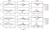Fig. 4. $c_{\mathrm{A}}^{\mathit{EB}}(k)$, $c_{\mathrm{A}}^{\mathit{TB}}(k)$, and $c_{\mathrm{A}}^{\mathit{TE}}(k)$ (first, second, and third column) for the ARs of category A (see Table 1) from the Northern hemisphere (top row) and Southern hemisphere (bottom row), using Eq. (4) with E and B being computed at λ2, λ3.

The inspection of the λ₃ bin (Fig. 4 second and fourth row) reveals that the peculiar sign reversal of EB correlations is absent for most ARs of category A. The sign of $c_{\mathrm{A}}^{\mathit{EB}}$ is consistent with our previous analysis, except for AR 11542, for which the sign is negative and opposite to that expected for an AR in the South. The signs of $c_{\mathrm{A}}^{\mathit{TB}}$ in this bin are also consistently negative (positive) in the North (South), as seen before. The same is true for $c_{\mathrm{A}}^{\mathit{TE}}$, which is positive in both hemispheres for most ARs. The sign reversal in the EB correlations for AR 11542 is due to a change in sign of E rather than B, if we take a close look at its TE correlations. For categories B and C, we see the same reversal of E to negative signs at λ₂ (not shown), except for ARs 12022 and 12387, where the amplitudes of the correlations are too low to discern a sign reversal. This indicates that, regardless of the categories of the ARs, E changes sign in the wavelength bins closest to or at the line core.

In Fig. 5, we show maps of E and B for two ARs. We have just seen that at λ₂, $c_{\mathrm{A}}^{\mathit{EB}}$ shows a reversed sign to positive (instead of negative) for an AR in the North, and we can infer that this sign reversal is due to a change in the sign of E. Figure 5e also shows a different (positive in this case) sign of E in the center of the AR compared to the other wavelength bins; cf. Figs. 5a,i,m. A similar behaviour can be seen for AR 11542 at λ₃; see Fig. 5k. There is a change in sign of E (positive again), which corresponds to a change in $c_{\mathrm{A}}^{\mathit{EB}}$ at λ₃; see Fig. 4. We find that from our sample of ARs, almost all ARs display a sign reversal of EB and TE at λ₂ and for one AR 11542 at λ₃. In the case of AR 11542, we found the spectral line to be red-shifted as compared to the other observations, which explains the sign reversal at λ₃ instead of λ₂. Thus, the mechanism causing the change in sign of E, can affect both wavelength bins, λ₂ or λ₃, depending on the Doppler shift of the spectral line.

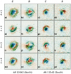Fig. 5. E and B maps for two ARs, computed from Stokes Q and U. The pattern of polarisation (green lines) have been scaled according to total linear polarisation signal ($\sqrt{Q^2+U^2}$). The colour scale is has been adjusted for each frame to easily see the positive (red) and negative (blue) values of E and B.

3.7. Tests for effects of Faraday rotation

Faraday rotation can change the different states of linear polarisation amongst themselves. Therefore, at certain wavelengths within a spectral line, depending on the magnetic field strength, the effects of Faraday rotation are the strongest. At these wavelengths, the maps of Stokes Q and U show a swirl-like pattern because of the different states of linear polarisation getting interchanged amongst themselves. B polarisation is sensitive to a curl-type pattern; therefore even a non-helical field, due to Faraday rotation, can give rise to a non-zero $c_{\mathrm{A}}^{\mathit{EB}}(k)$. This effect of Faraday rotation has been examined for dynamo-generated helical magnetic fields in a sphere (Brandenburg 2019) using Eq. (5).

In this section, we describe some simple tests we carried out to isolate the contribution of Faraday rotation from a non-helical magnetic field to the $c_{\mathrm{A}}^{\mathit{EB}}(k)$ correlation, when one computes it from Stokes Q and U near or at the line core. We started with a simple model of the solar atmosphere, the temperature stratification is based on the Harvard Smithsonian Reference Atmosphere (Gingerich et al. 1971). We introduced a magnetic field configuration which is constant with height in our model atmosphere; see Fig. 6. The field strength is decreasing outwards from the center following a Lorentzian profile, the inclination (γ) with respect to the line-of-sight was chosen in a way to make the magnetic field diverge away from the center, and similarly the azimuth was chosen such that the field was uniformly distributed in the transverse plane. We used STOPPRO (Solanki 1987), a numerical code which solves the RTE to synthesise the full Stokes vector for the 6173 Å Fe I absorption, with a spectral resolution of 5 mÅ. The spectra were synthesised for two distinct cases: one when such a magnetic configuration is at the disk center and another where it is at 30° in latitude. This latitude is roughly coinciding with the ones of the ARs we looked at in our analysis. The synthetic spectra were not degraded to account for instrumental effects and since we do not have any velocity gradients in our model, the spectra are symmetric about the line core. In both cases, we investigated different field strengths, keeping the inclination and azimuth of the magnetic field vector the same. We chose such a distribution of the magnetic field to mimic the magnetic field of a sunspot and to make sure that this field configuration is non-helical. This way, any non-zero correlation can only be attributed to Faraday rotation. Figure 7 shows the $c_{\mathrm{A}}^{\mathit{EB}}(k)$ at three different wavelengths, the one closest to the line core roughly falls in the λ₂ bin and the wavelength 105 mÅ away in the λ₁ bin. Since the spectra are symmetric, the $c_{\mathrm{A}}^{\mathit{EB}}(k)$ at λ₃, λ₄ is identical to the ones shown in the figure. We find the highest amplitudes of $c_{\mathrm{A}}^{\mathit{EB}}$ when the magnetic field configuration (regardless of the field strength) is at the disk center (solid lines in Fig. 7) as compared to when it is viewed from a position at 30° in latitude (dash-dotted lines in Fig. 7). In all cases, the maximum amplitude of $|c_{\mathrm{A}}^{\mathit{EB}}|$ for k between 0.1 to 1 is not higher than 0.2, but when it is computed from observations it is around 0.5 (see Fig. 1). Also, unlike observations, $c_{\mathrm{A}}^{\mathit{EB}}$ fluctuates around zero for these test cases. In terms of wavelength, the largest contributions from Faraday rotation to $c_{\mathrm{A}}^{\mathit{EB}}$ are, as expected, from wavelengths closest to the nominal line core.

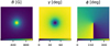Fig. 6. Magnetic field strength, inclination(γ) and azimuth (ϕ) for a simplistic sunspot-like configuration at the disk center.

Now we turn our attention to the sign reversal of E (and consequently of EB and TE). The E maps in Fig. 5 show a sign reversal at λ₂ for AR 12042 (panel e) and λ₃ for AR 11542 (panel k). It is tempting to relate this sign reversal to the effect of Faraday rotation, which is strongest at or close to the line core. Depending on the orbital velocity of SDO, this maximum can fall into wavelength bins λ₂ or λ₃. However, the E maps computed from the simple model of the solar atmosphere described above do not show any hint of a sign reversal. This means that either our model is too simple and not representative of the observations presented in Fig. 5, or that Faraday rotation is not the mechanism responsible for the sign reversal. We performed three experiments to examine this further.

In the first experiment we increased the complexity of the model by adding a filamentary fine structure directed radially outwards from the center of the synthetic spot, representative of a penumbra. But also this model failed to reproduce the sign reversal of E. In a second experiment we investigated the effect of a vertical gradient in the magnetic field parameters, which were neglected in the simple model described above. We computed the response functions of the Q and U profiles with respect to variations of the magnetic field strength in a typical umbral and penumbral atmosphere. The response functions describe the wavelength and height dependence of the Stokes parameters. We found the Q and U profiles to be sensitive over a ≈200 km thick layer above the optical depth unity surface with a rather uniform wavelength dependence. With typical gradients in a sunspot of ≈1 G km⁻¹ and the absence of a significant wavelength dependence, this height difference is too small to produce a large enough Faraday rotation and, therefore, it also does not explain the observed sign reversal in the E maps.

The third experiment is based on the data underlying Fig. 5. We applied the Milne-Eddington inversion code HeLIx+ (Lagg et al. 2004, 2009) to the HMI data of AR 12042 to retrieve its atmospheric parameters (e.g. magnetic field vector, line-of-sight velocity). The inversions reproduce the observed profiles reasonably well, the E and B maps computed from these fitted profiles are very similar to the observed E and B maps and show the observed sign change mostly at λ₂. In a next step, we used the atmospheric parameters from this inversion to compute synthetic Stokes profiles, neglecting the effect of Faraday rotation. The E and B maps computed from these profiles are very similar to the maps including Faraday rotation and show the sign change equally well. This proves that the observed sign change cannot be a result of Faraday rotation.

4. Conclusions

The study is motivated by an earlier work by Brandenburg et al. (2019), who demonstrated that the EB decomposition of linear polarisation can, under inhomogeneous conditions, be a proxy for magnetic helicity. However, they did not retrieve any significant non-zero EB correlations when they tested this proxy with solar observations from VSM/SOLIS. In this work, we looked at individual ARs from both hemispheres, observed with SDO/HMI, and not only recovered significant EB correlations, but also a systematic dependence of its sign on hemisphere. We found the sign of both EB and TB correlations to be consistent with that of small-scale magnetic helicity, that is, negative (positive) in the Northern (Southern) hemisphere. We note that this is opposite to what was reported in Brandenburg et al. (2019), based on numerical simulations of rotating convection. We also found that such parity-odd correlations (EB, TB), which are a good proxy for magnetic helicity, can be reliably computed from linear polarisation away from the line core of spectral lines. This minimises the influence of Faraday rotation on the various correlations and, since we use polarisation measurements directly, circumvents the π ambiguity. We found this to be true for the majority of the ARs we looked at (12 out of 18, category A). We also found 3 ARs (category B) that showed a reversed sign for the parity-odd correlations compared to what is predicted by theory, and 3 ARs (category C) that displayed no preference for a specific sign. As already alluded to above, the existence of ARs that display a reversed sign of parity-odd correlations (category B) may not be surprising since it has been demonstrated in previous studies (Pevtsov et al. 1995; Singh et al. 2018; Gosain & Brandenburg 2019) that there is a certain percentage of ARs that are in violation of the hemispheric sign rule for magnetic helicity. Proximity to the solar equator, complexity of the ARs, among others, are speculated to be the possible reasons behind these violations. Based on our present studies, the position of the AR on the solar disk or its complexity do not seem to be a factor in classifying an AR into categories A or B (see Table 1). However, our sample size is too small to draw more robust conclusions about this, so a more systematic study with a larger sample size is desirable.

We also computed the EB correlations from the transverse (b_θ, b_ϕ) components of the magnetic field vector (Sect. 3.5). The correlation $c_{\mathrm{A}}^{\mathit{EB}}(k)$ retrieved from this approximation matched the shape of the spectra retrieved directly from linear polarisation. A preference for a particular sign was less clear when $c_{\mathrm{A}}^{\mathit{EB}}$ was computed from the magnetic field, because the validity of Eq. (5) is questionable at AR latitudes. Nevertheless, it still gives us another confirmation that non-zero amplitudes of $c_{\mathrm{A}}^{\mathit{EB}}$ are not due to Faraday rotation, since the magnetic field is inferred after accounting for magneto-optical effects. Brandenburg (2019) also used the transverse components of the magnetic vector to compute EB correlations on a global scale. By using spin-2 spherical harmonics to compute E and B polarisations, and a heuristic approach to account for North-South sign change of magnetic helicity, he could successfully retrieve maximum power at the smallest wavenumbers. This is possibly due to the fact that the EB decomposition approach (regardless of it being computed from magnetic field or polarisation) is insensitive to the disambiguation, which can affect correlations at large scales, where field strengths are weak.

In Sect. 3.6, we looked at the different correlations computed from linear polarisation in wavelength bins close to the line core (λ₂, λ₃), suspecting significant influence of Faraday rotation on our inference. For the various correlations computed from these wavelength bins, both EB and TE correlations show a sign reversal, while the TB correlations do not. This indicates that the sign of E changes (and B does not change) closer to the line core. We mostly saw this reversal in the sign of E at λ₂, except for one AR where it happened at λ₃. However, this simply depends on the Doppler shift of the spectral line. We performed tests with a simple model of the solar atmosphere, and different iterations of it, to investigate the cause of this sign reversal of E and to reproduce it. Finally, we performed inversions of the observed profiles by HMI to infer the atmospheric parameters. From these computed synthetic spectra with and without Faraday rotation, we observed in both cases the sign reversal of E at λ₂, thus ruling out Faraday rotation as the cause of the sign reversal. It is still unclear what exactly causes this sign reversal of E near the line core, which occurs higher up in the atmosphere. E polarisation is linked to the topology of the magnetic field. Therefore, to understand this better, synthesising spectra from three-dimensional MHD simulations might be required to capture the changing magnetic field topology with height and the radiative transfer effects fully. This would help us narrow down the relation between the sign of E and the topology of the magnetic field, while still accounting for magneto-optic effects, mainly Faraday-rotation. The tests also revealed that the contributions to $c_{\mathrm{A}}^{\mathit{EB}}$ purely from Faraday rotation are relatively insignificant away from the nominal line core (Fig. 7). This agrees with the conclusions of Brandenburg (2019) who found that, provided the contributions from Faraday rotation are subdominant compared with the helicity contributions, one can detect magnetic helicity by using the EB decomposition. In the solar context, this is true away from the core of the spectral line. Therefore, we can safely infer magnetic helicity employing the EB decomposition. On the other hand, the spatial pattern of B polarisation also has an interesting feature in that it is predominantly bipolar (see Fig. 5) for almost all the inspected ARs at all wavelength bins. This is important since any spatial smoothing or averaging, even after multiplying with E or any other parity-even quantity, will result in cancellation.

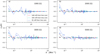Fig. 7. $c_{\mathrm{A}}^{\mathit{EB}}(k)$ calculated from Stokes Q and U for the synthetic test cases. The four panels correspond to different field strengths. The solid lines are for the spot-like configuration at the disk center. The dot-dashed lines are for the spot configuration at 30° latitude on the solar disk. For all the synthetic cases, we chose to assign the plate scale of HMI – hence the abscissa is in Mm−1.

The formalism to obtain E and B polarisation relies on linear polarisation, as it is directly borrowed from cosmology, wherein Thompson scattering only generates linear polarisation. However, in the solar context, the most frequently used diagnostic is the Zeeman effect, which also generates circular polarisation, and hence Stokes V is non-zero. Stokes V carries with it additional information about the directionality of the line-of-sight magnetic field. Except for the cases where we inferred Stokes Q and U from the components of the transverse magnetic field through Eq. (5), Stokes V has not been used in the present study. Including it is another possible next step to extend the present formalism to invoke Stokes V together with the EB decomposition.

Acknowledgments

We thank Nishant Singh (Pune, India) for useful discussions during the early phase of this project. Support through the NSF Astrophysics and Astronomy Grant Program, grant 1615100, and the Swedish Research Council, grant 2019-04234 (AB) are gratefully acknowledged. MJK acknowledges the support of the Academy of Finland ReSoLVE Centre of Excellence (Grant No. 307411). AP was funded by the International Max Planck Research School for Solar System Science at the University of Göttingen. This project has received funding from the European Research Council under the European Union’s Horizon 2020 research and innovation programme (project “UniSDyn”, grant agreement n:o 818665).

References

Appendix A: E and B decomposition

To study the polarisation signals of the cosmic microwave background (CMB), the linear polarisation signals generated through Thomson scattering are decomposed into E and B polarisations (Kamionkowski et al. 1997; Zaldarriaga & Seljak 1997). To demonstrate this decomposition here, we follow the convention and approach of Zaldarriaga & Seljak (1997), which arose out of the need to extract power spectra based on the rotationally invariant linear polarisation parameters. For a detailed derivation, we refer to the original article and the references therein. Here, we focus on the small-scale limit and discuss different conventions.

Stokes Q and U are frame-dependent quantities: a rotation of the polarisation basis (${\widehat{\mathit{e}}}_1$,${\widehat{\mathit{e}}}_2$) by an angle ϕ in the plane perpendicular to the propagation direction $\widehat{\mathit{n}}$ transforms Q and U as

$$\begin{array}{c}\hfill {(Q\pm iU)}^{\prime }=e^{\mp 2i\varphi }(Q\pm iU)(\widehat{\mathit{n}}),\end{array}$$(A.1)

with ${\widehat{\mathit{e}}}_1\prime =cos\varphi {\widehat{\mathit{e}}}_1+sin\varphi {\widehat{\mathit{e}}}_2$ and ${\widehat{\mathit{e}}}_2\prime =-sin\varphi {\widehat{\mathit{e}}}_1+cos\varphi {\widehat{\mathit{e}}}_2$. For a harmonic analysis of the Q + iU over the entire sphere and given the rotational dependence of Q and U, it is appropriate to expand them in a spin-weighted basis as

$$\begin{array}{c}\hfill (Q\pm iU)(\widehat{\mathit{n}})={\displaystyle \sum _{\mathit{lm}}{a}_{\mathit{lm}}^{\pm 2}{}_{\pm 2}{Y}_{\mathit{lm}}(\widehat{\mathit{n}}),}\end{array}$$(A.2)

where _sY_lm are spin-weighted spherical harmonic functions for each integer s with |s| ≤ l, which transform under rotation. For convenience, we can define linear combinations of the above coefficients, such as

$$\begin{array}{c}\hfill a_{\mathit{lm}}^E=-(a_{\mathit{lm}}^2+a_{\mathit{lm}}^{-2})/2\mathrm{and}{a}_{\mathit{lm}}^B=-(a_{\mathit{lm}}^2-a_{\mathit{lm}}^{-2})/2i.\end{array}$$(A.3)

Here one can also notice the parity-even and parity-odd properties of E and B; E remains unchanged, whereas B changes sign.

In this paper, we work within the confines of the small-scale limit. That is, for a high enough degree of spherical harmonics, we can neglect the curvature of the sphere and consider it as a plane normal to e_z. In this limit, spin-weighted spherical harmonics can be approximated in terms of exponentials as

$$\begin{array}{cc}& {}_2{Y}_{\mathit{lm}}={\left[\frac{(l-2)!}{(l+2)!}\right]}^{1/2}{ð}^2{Y}_{\mathit{lm}}⟶\frac{1}{2\pi }\frac{1}{l^2}{ð}^2{e}^{i\mathit{k}·\mathit{x}},\hfill \\ \hfill & {}_{-2}{Y}_{\mathit{lm}}={\left[\frac{(l-2)!}{(l+2)!}\right]}^{1/2}{\overline{ð}}^2{Y}_{\mathit{lm}}⟶\frac{1}{2\pi }\frac{1}{l^2}{\overline{ð}}^2{e}^{i\mathit{k}·\mathit{x}},\hfill \end{array}$$(A.4)

where x is a vector in the plane normal to e_z and K is its counterpart in Fourier-space, where k_x + ik_y = ke^iϕ_k. Furthermore, ð and $\overline{ð}$ are spin raising and spin lowering operators (see Goldberg et al. 1967).

Thus, invoking the small-scale approximation (A.4) and using the linear combinations defined in Eq. (A.3), we can obtain the following expression from Eq. (A.2) (see Zaldarriaga & Seljak 1997)

$$\begin{array}{c}\hfill \stackrel{\sim }{Q}+i\stackrel{\sim }{U}=(\stackrel{\sim }{E}+i\stackrel{\sim }{B})e^{2i{\varphi }_k}.\end{array}$$(A.5)

The relation can also be written differently in terms of the components of the unit vector $\widehat{\mathit{k}}=\mathit{k}/k$ as

$$\begin{array}{c}\hfill (\stackrel{\sim }{E}+i\stackrel{\sim }{B})={({\widehat{k}}_x-i{\widehat{k}}_y)}^2(\stackrel{\sim }{Q}+i\stackrel{\sim }{U}),\end{array}$$(A.6)

which is the relation used in the present paper.

The linear combinations in Eq. (A.3) were defined according to the convention chosen by Zaldarriaga & Seljak (1997) and this is the sign convention we follow in this study. However, there exists another sign convention followed by Durrer (2008) and Brandenburg (2019), wherein these linear combinations are defined as

$$\begin{array}{c}\hfill {\stackrel{\sim }{a}}_{\mathit{lm}}^E=(a_{\mathit{lm}}^2+a_{\mathit{lm}}^{-2})/2\mathrm{and}{\stackrel{\sim }{a}}_{\mathit{lm}}^B=(a_{\mathit{lm}}^2-a_{\mathit{lm}}^{-2})/2i.\end{array}$$(A.7)

As a result of this convention, Eq. (A.6) acquires an additional minus sign. The sign convention chosen by Zaldarriaga & Seljak (1997) is such that positive (negative) values of E generate a tangential (radial) pattern (see Fig. A.1a, b) and in the case of B polarisation, positive (negative) values of B generate an anticlockwise (clockwise) inward spiralling pattern of polarisation. A consequence of the different sign convention of Durrer (2008) is that negative values of E now generate a tangential pattern of polarisation (see Figs. A.1c, d).

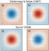Fig. A.1. Top row: illustration of the pattern of polarisation generated by positive (red) and negative (blue) values of E following the sign convention of Zaldarriaga & Seljak (1997). Bottom row: same as in top row, but for the sign convention of Durrer (2008).

Appendix B: Examples

We performed tests with a magnetic field configuration following Sect. 2.3 of Brandenburg et al. (2019). The magnetic field was defined as a sum of gradient- and curl-type fields:

$$\begin{array}{cc}& \mathit{b}(x,y)=\mathit{F}+\mathit{G},\hfill \end{array}$$(B.1)

$$\begin{array}{cc}& F_i(x,y)={\partial }_{i}f,G_i(x,y)={ϵ}_{\mathit{ij}}{\partial }_{j}g,\hfill \end{array}$$(B.2)

$$\begin{array}{cc}& f=f_{0}cos(kx)cos(ky),g=g_{0}cos(kx)cos(ky).\hfill \end{array}$$(B.3)

This b vector only provides the planar projection of a fully three-dimensional solenoidal magnetic field. With this, we have the freedom to choose a vector field with a given wavenumber k. With such a field in a simple atmosphere, we can synthesise the full Stokes vector and compute E and B from Stokes Q and U. The goal is to exploit the E and B decomposition of linear polarisation to infer the characteristics of the original vector field (be it the wavenumber or the handedness of the vector field) directly from the polarisation signal. We chose three cases: one with a b field corresponding to a pure E polarisation (f₀ = 1, g₀ = 0, Fig. B.1a), a second case with a b field corresponding to pure B polarisation (f₀ = 1, g₀ = 1, Fig. B.1b), and lastly, a b field, which would result in both E and B polarisations (f₀ = cos θ, g₀ = ± sin θ, Fig. B.1c) but of opposite handednesses by changing the sign of g₀. In all three cases, we repeated the experiments for different wavenumbers, k = k₀ and k = 10k₀. As described before, we synthesised Stokes Q and U for all these cases and computed the relevant shell-integrated spectra. We show c^EE(k) for the case of pure E polarisation, c^BB(k) for pure B polarisation, and c^EB(k) for the third case where both E and B are non-zero.

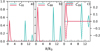Fig. B.1. $c_{\mathrm{A}}^{\mathit{EE}}(k)$, $c_{\mathrm{A}}^{\mathit{BB}}(k)$, and $c_{\mathrm{A}}^{\mathit{EB}}(k)$ calculated from Stokes Q and U for case a: pure E polarisation, case b: pure B polarisation, and case c: non-zero E and B polarisations, respectively. The red curve is for k = k0 and the blue curve for k = 10k0. The dotted curve in panel c, corresponds to a different handedness of the original b field resulting in $c_{\mathrm{A}}^{\mathit{EB}}(k)$ of an opposite sign.

In all cases, we retrieve maximum amplitudes in the corresponding normalised correlation spectra at the chosen wavenumbers to define the b fields with k = k₀ and k = 10k₀. For the last case (Fig. B.1c) we also retrieve different signs of c^EB(k) for the opposite handednesses of the vector fields. This is due to the B polarisation changing sign under a parity transformation. For k = 10k₀, we also retrieve a secondary peak of lower amplitude. This is probably an artifact resulting from the spectral synthesis, wherein we assume a simplified atmosphere with these idealised magnetic fields.

All Tables

All Figures

	Fig. 1. $c_{\mathrm{A}}^{\mathit{EB}}(k)$, $c_{\mathrm{A}}^{\mathit{TB}}(k)$, and $c_{\mathrm{A}}^{\mathit{TE}}(k)$ (first, second, and third column) for the ARs of category A from the Northern hemisphere (top row) and Southern hemisphere (bottom row) (see Table 1), using Eq. (4) with E and B being computed at λ0, λ1, λ4, λ5.
In the text

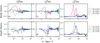	Fig. 2. Similar to Fig. 1, but the ARs of categories B (solid lines) and C (dashed lines).
In the text

	Fig. 3. $c_{\mathrm{A}}^{\mathit{EB}}(k)$ for ARs of categories A (left column), B (right column, solid lines), and C (right column, dashed lines), with E and B being calculated from the components of the magnetic field vector. The curves for $c_{\mathrm{A}}^{\mathit{EB}}(k)$ are smoothed in logarithmically spaced bins, for better visibility.
In the text

	Fig. 4. $c_{\mathrm{A}}^{\mathit{EB}}(k)$, $c_{\mathrm{A}}^{\mathit{TB}}(k)$, and $c_{\mathrm{A}}^{\mathit{TE}}(k)$ (first, second, and third column) for the ARs of category A (see Table 1) from the Northern hemisphere (top row) and Southern hemisphere (bottom row), using Eq. (4) with E and B being computed at λ2, λ3.
In the text

	Fig. 5. E and B maps for two ARs, computed from Stokes Q and U. The pattern of polarisation (green lines) have been scaled according to total linear polarisation signal ($\sqrt{Q^2+U^2}$). The colour scale is has been adjusted for each frame to easily see the positive (red) and negative (blue) values of E and B.
In the text

	Fig. 6. Magnetic field strength, inclination(γ) and azimuth (ϕ) for a simplistic sunspot-like configuration at the disk center.
In the text

Fig. 7. $c_{\mathrm{A}}^{\mathit{EB}}(k)$ calculated from Stokes Q and U for the synthetic test cases. The four panels correspond to different field strengths. The solid lines are for the spot-like configuration at the disk center. The dot-dashed lines are for the spot configuration at 30° latitude on the solar disk. For all the synthetic cases, we chose to assign the plate scale of HMI – hence the abscissa is in Mm−1.

In the text

	Fig. A.1. Top row: illustration of the pattern of polarisation generated by positive (red) and negative (blue) values of E following the sign convention of Zaldarriaga & Seljak (1997). Bottom row: same as in top row, but for the sign convention of Durrer (2008).
In the text

Fig. B.1. $c_{\mathrm{A}}^{\mathit{EE}}(k)$, $c_{\mathrm{A}}^{\mathit{BB}}(k)$, and $c_{\mathrm{A}}^{\mathit{EB}}(k)$ calculated from Stokes Q and U for case a: pure E polarisation, case b: pure B polarisation, and case c: non-zero E and B polarisations, respectively. The red curve is for k = k0 and the blue curve for k = 10k0. The dotted curve in panel c, corresponds to a different handedness of the original b field resulting in $c_{\mathrm{A}}^{\mathit{EB}}(k)$ of an opposite sign.

In the text

References

- Berger, M. A. 1984, Geophys. Astrophys. Fluid Dynam., 30, 79 [Google Scholar]
- Berger, M. A., & Field, G. B. 1984, J. Fluid Mech., 147, 133 [NASA ADS] [CrossRef] [Google Scholar]
- Blackman, E. G. 2015, Space Sci. Rev., 188, 59 [Google Scholar]
- Blackman, E. G., & Brandenburg, A. 2003, ApJ, 584, L99 [NASA ADS] [CrossRef] [Google Scholar]
- Bobra, M. G., Sun, X., Hoeksema, J. T., et al. 2014, Sol. Phys., 289, 3549 [NASA ADS] [CrossRef] [Google Scholar]
- Borrero, J. M., Tomczyk, S., Kubo, M., et al. 2011, Sol. Phys., 273, 267 [Google Scholar]
- Brandenburg, A. 2019, ApJ, 883, 119 [CrossRef] [Google Scholar]
- Brandenburg, A., & Subramanian, K. 2005, Phys. Rep., 417, 1 [NASA ADS] [CrossRef] [Google Scholar]
- Brandenburg, A., Sokoloff, D., & Subramanian, K. 2012, Space Sci. Rev., 169, 123 [NASA ADS] [CrossRef] [Google Scholar]
- Brandenburg, A., Petrie, G. J. D., & Singh, N. K. 2017, ApJ, 836, 21 [Google Scholar]
- Brandenburg, A., Bracco, A., Kahniashvili, T., et al. 2019, ApJ, 870, 87 [NASA ADS] [CrossRef] [Google Scholar]
- del Toro Iniesta, J. C., & Ruiz Cobo, B. 2016, Liv. Rev. Sol. Phys., 13, 4 [Google Scholar]
- Durrer, R. 2008, The Cosmic Microwave Background (Cambridge University Press) [CrossRef] [Google Scholar]
- Gingerich, O., Noyes, R. W., Kalkofen, W., & Cuny, Y. 1971, Sol. Phys., 18, 347 [Google Scholar]
- Goldberg, J. N., MacFarlane, A. J., Newman, E. T., Rohrlich, F., & Sudarshan, E. G. 1967, J. Math. Phys., 8, 2155 [NASA ADS] [CrossRef] [Google Scholar]
- Gosain, S., & Brandenburg, A. 2019, ApJ, 882, 80 [NASA ADS] [CrossRef] [Google Scholar]
- Kahniashvili, T., & Ratra, B. 2005, Phys. Rev. D, 71, 103006 [NASA ADS] [CrossRef] [Google Scholar]
- Kahniashvili, T., Maravin, Y., Lavrelashvili, G., & Kosowsky, A. 2014, Phys. Rev. D, 90, 083004 [NASA ADS] [CrossRef] [Google Scholar]
- Kamionkowski, M., Kosowsky, A., & Stebbins, A. 1997, Phys. Rev. Lett., 78, 2058 [NASA ADS] [CrossRef] [Google Scholar]
- Kosowsky, A., & Loeb, A. 1996, ApJ, 469, 1 [NASA ADS] [CrossRef] [Google Scholar]
- Krause, F., & Rädler, K.-H. 1980, Mean-field Magnetohydrodynamics and Dynamo Theory (Oxford: Pergamon Press) [Google Scholar]
- Lagg, A., Woch, J., Krupp, N., & Solanki, S. K. 2004, A&A, 414, 1109 [NASA ADS] [CrossRef] [EDP Sciences] [Google Scholar]
- Lagg, A., Ishikawa, R., Merenda, L., et al. 2009, in The Second Hinode Science Meeting: Beyond Discovery-Toward Understanding, eds. B. Lites, M. Cheung, T. Magara, J. Mariska, K. Reeves, et al., Astron. Soc. Pacific Conf. Ser., 415, 327 [Google Scholar]
- Landi Degl’Innocenti, E., & Landi Degl’Innocenti, M. 1985, Sol. Phys., 97, 239 [NASA ADS] [CrossRef] [Google Scholar]
- Leka, K. D., Barnes, G., Crouch, A. D., et al. 2009, Sol. Phys., 260, 83 [Google Scholar]
- Metcalf, T. R. 1994, Sol. Phys., 155, 235 [Google Scholar]
- Metcalf, T. R., Leka, K. D., Barnes, G., et al. 2006, Sol. Phys., 237, 267 [Google Scholar]
- Moffatt, H. K. 1978, Magnetic Field Generation in Electrically Conducting Fluids (Cambridge University Press) [Google Scholar]
- Parker, E. N. 1955, ApJ, 122, 293 [NASA ADS] [CrossRef] [Google Scholar]
- Pevtsov, A. A., Canfield, R. C., & Metcalf, T. R. 1995, ApJ, 440, L109 [NASA ADS] [CrossRef] [Google Scholar]
- Pogosian, L., Vachaspati, T., & Winitzki, S. 2002, Phys. Rev. D, 65, 083502 [NASA ADS] [CrossRef] [Google Scholar]
- Roberts, P. H., & Soward, A. M. 1975, Astron. Nachr., 296, 49 [NASA ADS] [CrossRef] [Google Scholar]
- Scannapieco, E. S., & Ferreira, P. G. 1997, Phys. Rev. D, 56, R7493 [NASA ADS] [CrossRef] [Google Scholar]
- Schou, J., Scherrer, P. H., Bush, R. I., et al. 2012, Sol. Phys., 275, 229 [Google Scholar]
- Scóccola, C., Harari, D., & Mollerach, S. 2004, Phys. Rev. D, 70, 063003 [NASA ADS] [CrossRef] [Google Scholar]
- Seehafer, N. 1990, Sol. Phys., 125, 219 [NASA ADS] [CrossRef] [Google Scholar]
- Seehafer, N. 1996, Phys. Rev. E, 53, 1283 [Google Scholar]
- Seljak, U. 1997, ApJ, 482, 6 [Google Scholar]
- Seljak, U., & Zaldarriaga, M. 1997, Phys. Rev. Lett., 78, 2054 [NASA ADS] [CrossRef] [Google Scholar]
- Singh, N. K., Käpylä, M. J., Brandenburg, A., et al. 2018, ApJ, 863, 182 [Google Scholar]
- Solanki, S. K. 1987, PhD Thesis, ETH Zürich, Switzerland [Google Scholar]
- Yousef, T. A., & Brandenburg, A. 2003, A&A, 407, 7 [NASA ADS] [CrossRef] [EDP Sciences] [Google Scholar]
- Zaldarriaga, M., & Seljak, U. 1997, Phys. Rev. D, 55, 1830 [Google Scholar]
- Zhang, H., Brandenburg, A., & Sokoloff, D. D. 2014, ApJ, 784, L45 [NASA ADS] [CrossRef] [Google Scholar]
- Zhang, H., Brandenburg, A., & Sokoloff, D. D. 2016, ApJ, 819, 146 [NASA ADS] [CrossRef] [Google Scholar]