| Issue |
A&A
Volume 641, September 2020
|
|
|---|---|---|
| Article Number | A19 | |
| Number of page(s) | 22 | |
| Section | Planets and planetary systems | |
| DOI | https://doi.org/10.1051/0004-6361/201937152 | |
| Published online | 01 September 2020 | |
Discrete element modeling of boulder and cliff morphologies on comet 67P/Churyumov-Gerasimenko
1
Institute of Physics and Astronomy, University of Potsdam,
Karl-Liebknecht-Str. 24–25,
14476
Potsdam,
Germany
e-mail: dakappel@uni-potsdam.de
2
Institute of Planetary Research, German Aerospace Center (DLR),
Rutherfordstr. 2,
12489
Berlin,
Germany
Received:
20
November
2019
Accepted:
10
July
2020
Context. Even after the Rosetta mission, some of the mechanical parameters of comet 67P/Churyumov-Gerasimenko’s surface material are not yet well constrained. These parameters are needed to improve our understanding of cometary activity or for planning sample return missions.
Aims. We study some of the physical processes involved in the formation of selected surface features and investigate the mechanical and geometrical parameters involved.
Methods. Applying the discrete element method (DEM) in a low-gravity environment, we numerically simulated the surface layer particle dynamics involved in the formation of selected morphological features. The material considered is a mixture of polydisperse ice and dust spheres with inter-particle forces given by the Hertz contact model, translational friction, rolling friction, cohesion from unsintered contacts, and optionally due to bonds from ice sintering. We determined a working set of parameters that enables the simulations to be reasonably realistic and investigated morphological changes due to modifications thereof.
Results. The selected morphological features are reasonably well reproduced using model materials with a tensile strength on the order of 1–10 Pa. Increasing the diameters of the spherical particles decreases the material strength, and increasing the friction leads to a more brittle but somewhat stronger material. High friction is required to make the material sufficiently brittle to match observations, which points to the presence of very rough, even angular particles. Reasonable seismic activity does not suffice to trigger the collapses of cliffs without material heterogeneities or structural defects.
Conclusions. DEM modeling can be a powerful tool to investigate mechanical parameters of cometary surface material. However, many uncertainties arise from our limited understanding of particle shapes, spatial configurations, and size distributions, all on multiple length scales. Further numerical work, in situ measurements, and sample return missions are needed to better understand the mechanics of cometary material and cometary activity.
Key words: comets: general / comets: individual: 67P/Churyumov-Gerasimenko / methods: numerical
© ESO 2020
1 Introduction
Remote sensing data of cometary nuclei have revealed a wealth of morphologic features that cover the surfaces of comets (Sunshine et al. 2016; El-Maarry et al. 2019). These include features unique to comets, such as pits (Vincent et al. 2015) and quasi-circular depressions (Brownlee et al. 2004), but they also encompass features known from other planetary bodies, such as mass-wasting deposits (Thomas et al. 2015a), boulder fields (Pajola et al. 2015), and sedimentary deposits (Thomas et al. 2015b). Morphologic features and the processes that form them are manifestations of the mechanical properties of the cometary material under the influence of a relatively low surface acceleration (~2 × 10⁻⁴ m s−2, Groussin et al. 2015), an effect of cohesive forces that is more pronounced than in our natural terrestrial environment (Scheeres et al. 2010), and the activity generated by sublimation of ices at smaller heliocentric distances. These features have the potential to reveal information on the mechanical properties of the cometary material which is indispensable for a wide range of research involving the modeling of activity, outbursts, thermal alterations, and potential sample- return techniques.
The mechanical properties of the most thoroughly studied comet 67P/Churyumov-Gerasimenko (hereafter 67P) have been investigated by a variety of instruments onboard the Rosetta spacecraft and its lander Philae. The nucleus of 67P measures approximately 4.3 km by 4.1 km at its longest and widest dimensions, respectively, and consists of a larger and a smaller lobe connected by a narrower neck (Sierks et al. 2015). The evaluation of in situ data acquired on the nucleus surface (Knapmeyer et al. 2018; Spohn et al. 2015) and of remote sensing data from kilometer-scale (Sierks et al. 2015; Capaccioni et al. 2015; Fornasier et al. 2015) and centimeter-scale (Mottola et al. 2015; Bibring et al. 2015) distances have revealed the presence of highly complex processes shaping the comet’s surface and near subsurface. For example, the southern hemisphere of comet 67P is mainly composed of bare consolidated material while the northern hemisphere is extensively covered by airfall particles (El-Maarry et al. 2015, 2016, 2017). This dichotomy is caused by inhomogeneous energy input introduced by seasonal effects, which result in higher erosion rates in the south and airfall particle deposition in the north (Keller et al. 2015, 2017).
The consolidated surface layer mainly observed in 67P’s southern hemisphere is probably extremely tough with a uniaxial compressive strength of >2 MPa (Spohn et al. 2015), presumably as a result of sintering of water ice components of the surface layer material, but the compressive strength of the granular airfall material covering the northern hemisphere is only ~1–3 kPa with a shear strength of 4–30 Pa (Biele et al. 2015; Groussin et al. 2015; Basilevsky et al. 2016). The size and arrangement of fracture polygons on the consolidated surfaces also hint at a strength in the MPa range (Auger et al. 2018). The thickness of a sintered layer is related to the diurnal and seasonal thermal skin depths, which are of the order of 1–2 cm and 1 m, respectively (Gulkis et al. 2015). In agreement with these findings, the accelerometers onboard the Philae lander measured the thickness of the consolidated layer at the Abydos landing site, and a value of 10–50 cm was retrieved (Knapmeyer et al. 2018). Below this layer, the cometary material is assumed to be unaffected by insolation and should therefore be pristine (Groussin et al. 2015). Observations by Rosetta seem to suggest that the pristine bulk cometary material is composed of small pebbles ranging from millimeter to centimeter scales (Fulle et al. 2016; Blum et al. 2017). These pebbles are built of individual, smaller, micron-scale dust grains (Fulle et al. 2015; Mannel et al. 2016) and volatiles that may sublime when close to the sufficiently illuminated comet surface (Blum et al. 2017).
Estimates of the tensile strength of the pristine cometary material on a larger scale have been derived from geometrical dimensions of overhangs in the presence of the local surface acceleration and are found to be on the order of 10 Pa (Groussin et al. 2015; Attree et al. 2018). Additional estimates based on stresses introduced by the self-gravity of the whole bilobed comet reveal a comparable internal strength between 10 Pa and 70 Pa (Hviid et al. 2016, Hviid et al., priv. comm.). The tensile strength could also be constrained by the Deep Impact cratering experiment on comet Tempel 1 and has been reported to be less than 12 kPa (Holsapple & Housen 2007).
Further mechanical properties of the consolidated surface material on 67P have been derived with the accelerometers onboard the Philae lander, which allow a confinement of the shear modulus to 3.6–346 MPa and of Young’s modulus to 7.2–980 MPa (Knapmeyer et al. 2018). The average density of 67P was determined as ~0.5 g cm−3 (Jorda et al. 2016; Preusker et al. 2017) leading to a bulk porosity of 70–75% assuming a dust-to-ice-mass ratio of 4 ± 2 (Rotundi et al. 2015), which is highly comparable to the porosity of 75–85% inferred from CONSERT radar measurements (Kofman et al. 2015).
Despite the low strength, density, and gravitational acceleration on cometary surfaces, the strength-to-gravity ratio is similar to that of weak rocks on Earth (e.g. siltstone) (Groussin et al. 2015). Therefore, well-known gravitationally influenced processes on Earth, such as cliff collapses and the subsequent deposition of boulders on intermediate slopes, are also abundant on 67P (Fig. 1). In particular, the recent collapse of the Aswan cliff on 67P has attracted much attention because it revealed pristine material enriched in water ice at the freshly exposed escarpment (Pajola et al. 2017). The collapse of the approximately 134 m-high cliff generated talus material and debris, which comprises a large number of boulders (Pajola et al. 2017; Pajola et al. 2016). The largest boulder has a size of 25.5 m and is located on a relatively flat slope of less than 10°. Generally, the sizes of deposited boulders on 67P decrease with increasing slope (Pajola et al. 2016; Groussin et al. 2015), and the largest boulders are located in the comet’s gravitational lows (Imhotep and Hapi morphological regions; Thomas et al. 2015a) with diameters up to about 50 m. Boulders located in the neck region of 67P (Hapi region) possibly dropped from a maximum height of approximately 900 m (Thomas et al. 2015a). The survival of these relatively large boulders from falls of such heights again constrains the mechanical properties of the involved material.
Due to the limited temporal coverage of observations at given surface locations, dynamical processes like cliff collapses have not been observed themselves, but in the best cases observations were made before and after they happened. Other processes causing slowbut continuous changes of the local surface morphology like dust movement (dunes, aeolian-like structures, burying or excavation of consolidated structures by dust) or the development of fracture networks have mainly been observed with long time gaps.
To complement the available measurements and improve our general understanding of the mechanical properties and dynamic processes oncomets, numerical simulations can help to constrain some of the micro- and macro-mechanical parameters, for example by excluding certain parameter ranges or combinations incompatible with the development of various observed morphological features. The discrete element method (DEM) is a widely accepted method for modeling granular and discontinuous materials that consist of separate, discrete particles, a well-suited analog for the pebbles assumed to make up the pristine cometary material.
The DEM has also been used to simulate the dynamics of atoms and molecules, granular matter, bulk materials, and rocks. In the field of planetary science, DEM modeling has been used to study the formation, evolution, and surface properties of planetary bodies, including small bodies with weak surface materials and at low gravity such as asteroids and comets. For example, it has been used to simulate impact processes on the asteroids Eros and Itokawa to explain the origin of exposed boulders on their surfaces via the Brazil nut effect (Tancredi et al. 2012), the removal of surface materials on asteroids by strong centrifugal forces resulting from rapid rotation (Hirabayashi et al. 2015), and catastrophiccollisional disruptions of planetesimals and reaccumulation of their fragments to explain the formation and the bilobate shape of several comets including 67P (Schwartz et al. 2018). The DEM has also been used to address engineering problems such as hopping mechanisms to relocate landers on asteroids (Cheng et al. 2019) and techniques to sample material from asteroid surfaces (Cheng et al. 2017). However, DEM modeling has not yet been widely used to study the surface morphology or mechanical properties of cometary material – a material in a low-gravity environment that, in addition to dust, consists of ices, and where the ices may form sinter bonds and sublime.
Our overall aim in studying the mechanical properties of cometary surfaces and nuclei is to provide reliable data needed to understand the development of the coma (e.g., dust lifting), to assess the impact scenarios on the nucleus itself or of a comet on the Earth for example, to design mitigation schemes to change a comet’s ephemerides to avoid the latter, to design sample-return procedures (Squyres et al. 2018; Küppers et al. 2009), and so on. Depending on whether the nucleus is a so-called rubble pile with or without large voids or a mechanically homogeneous dust–ice mixture, mechanical interactions can turn out very differently. In the same way, it can make a large difference if the nucleus has a tough meter-scale surface layer that extends globally or is locally confined, has large tough or weak boulders, or is entirely built from fluffy particle agglomerates. This can render a sample-return procedure unsuccessful or can decide which method is to be employed for an ephemerides modification required to prevent a potential impact on Earth.
In particular, we investigate in the present work the dropping of larger boulders from small heights and collapses of cliffs. For this purpose, we aim to reproduce such events with DEM modeling of corresponding suitable simulation scenarios using the example of comet 67P. Since the modeling cannot capture the full real-world complexity, our immediate aim is to study some of the physical processes involved in the formation of these features and to find a working set of parameters that enables the simulations to be reasonably realistic. The simulation scenarios are then used as starting points for parameter sensitivity studies to constrain mechanical properties, contact forces, particle sizes, and so on, of the surface-layer material.
In Sect. 2 we provide details of our numerical DEM modeling. The basic investigated simulation scenarios are introduced in Sect. 3, and the simulation outcomes and changes when varying their setups are presented and discussed in Sect. 4. Finally, conclusions and an outlook are given in Sect. 5.
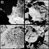 |
Fig. 1 Examples of morphologic features on comet 67P as imaged by the OSIRIS narrow-angle camera (Keller et al. 2007). (a) Hathor cliff with boulders accumulating at the airfall-covered foot of the cliff. The consolidated tough material of the cliff supports an escarpment height of about 900 m. The largest boulders are approximately 50 m across. (b) Pre-collapse Aswan plateau and cliff site with smooth airfall deposits, consolidated wall material, and debris with boulders at the cliff foot (center left). The shadowed pit in the top left of the image is approximately 200 m across. (c) Foot of a collapsed debris field populated with boulders up to 10–15 m across. (d) Debris deposits superimposing an apparently smooth region of small airfall particles. Bare consolidated and airfall-covered terrains alternate spatially. The boulder deposit in the upper left and the airfall-covered plateau in the center of the image are each approximately 500 m wide. Figure tags: (a) NAC_ 2014-09-29T08.52.08.332Z_ID30_1397549001_F41, (b) NAC_2014-09-29T16.10.04.817Z_ID30_1397549000_F16, (c) NAC_2016-08-03T07.28.34.758Z_ID30_1397549000_F22, (d) NAC_2014-09-13T23.29.22.367Z_ID30_1397549001_F41. Credits: ESA/Rosetta/MPS for OSIRIS Team MPS/UPD/LAM/IAA/SSO/INTA/UPM/DASP/IDA. |
2 Numerical modeling
The dynamics of the granular cometary surface material are modeled with the open-source DEM simulation code LIGGGHTS (Kloss et al. 2012) which is capable of parallel processing. Generally, we assume the particles to be represented by polydisperse spheres consisting either of dust or of water ice. The spheres interact according to the Hertz contact model (Sect. 2.1) and additionally are subject to translational friction (Sect. 2.1), rolling friction (Sect. 2.2), and ambient surface acceleration. In addition to unsintered cohesive contacts (Sect. 2.3), bonds from ice sintering can be introduced (Sect. 2.4) that break when the interparticle stresses exceed certain threshold values. This way, we can also model the hard consolidated terrain that was found in many places on the surface of 67P and may result from water-ice sintering. To enable the simulation of macroscopic scenarios with relatively small particles, we apply the coarse-graining technique (Bierwisch et al. 2009) (Sect. 2.5). Table 1 provides an overview of the employed symbols and typing notations.
2.1 Hertz contact model
Using the discrete element method (Cundall & Strack 1979) to model the dynamics of granular matter, Newton’s equations of motion,
![\begin{align*} &m_i\, \dot{\vec v}_i=\vec F_i\nonumber\\[2pt] &\underline{I_i}\, \dot{\vec\omega}_i=\vec M_i, \end{align*}](/articles/aa/full_html/2020/09/aa37152-19/aa37152-19-eq1.png) (1)
(1)
have to be solved for N particles with masses mi, inertia tensors  , center of mass positions ri, velocities vi, angular velocities ωi, forces Fi, and torques Mi, where subscript i is a counting index with i ∈{1, ⋯, N}. The solution is performed by explicit time integration with fixed time-step Δt using the velocity Verlet method (Swope et al. 1982) that achieves a global error of order two,
![\begin{align*} &\vec r_i\left(t+\Delta t\right)=\vec r_i\left(t\right)+\vec v_i\left(t\right)\Delta t+\frac{\vec F_i\left(t\right)}{2m_i}\Delta t^2\nonumber\\ &\vec v_i\left(t+\Delta t\right)=\vec v_i\left(t\right)+\frac{\vec F_i\left(t\right)+\vec F_i\left(t+\Delta t\right)}{2m_i}\Delta t\nonumber\\ &\vec \omega_i\left(t+\Delta t\right)=\vec\omega_i\left(t\right)+\frac{\underline{I_i}^{-1}\left[\vec M_i\left(t\right)+\vec M_i\left(t+\Delta t\right)\right]}{2}\Delta t. \end{align*}](/articles/aa/full_html/2020/09/aa37152-19/aa37152-19-eq3.png) (2)
(2)
The net force Fi acting on a given particle can be written as a sum of external forces Fext,i and of forces arising from interactions with other particles Fij,
 (3)
(3)
Here, we only consider the force due to the surface acceleration of the nucleus, Fext,i = mi g, and mechanical forces between contacting particles as listed in the introduction paragraph of Sect. 2. In particular, we do not consider gravity between particles, solar radiation pressure, or electrostatic forces.
In order to efficiently check for interactions between particles, neighbor lists, which store all particle pairs within a given cutoff distance, are used and only updated after several time-steps. Typically, the larger the cutoff distance, the less often neighbor lists need to be updated, but at every time-step more pairs must be checked for possible interactions. The time-steps were set to be just shorter than 10% of the minimum of Rayleigh time and Hertz time, which proved to lead to a stable time integration, but exemplarily we also test 3%.
The Hertz (H) contact force between two particles is computed as the sum of the normal (n) and tangential (t) forces at the contact point (Kloss et al. 2012),
 (4)
(4)
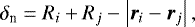
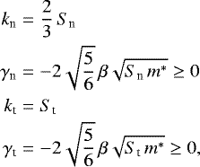
which is a nonlinear spring-dashpot model consisting of an elastic (Hertz 1882) and a viscous/dissipative part. kn and kt are the elastic parameters for normal and tangential contact, and γn and γt the normal and tangential damping parameters that govern the damping forces resulting at the relative normal and tangential velocities of the surfaces at the contact point, vn and vt, which are given by
![\begin{align*} &\vec v=\left(\dot{\vec r}_i-\vec\omega_i\times R_i\,\vec n\right) -\left(\dot{\vec r}_j+\vec\omega_j\times R_j\,\vec n\right)\nonumber\\[2pt] &\vec v_{\textrm{n}}=\left(\vec v\cdot\vec n\right)\vec n\nonumber\\[2pt] &\vec v_{\textrm{t}}=\vec v-\vec v_{\textrm{n}}, \end{align*}](/articles/aa/full_html/2020/09/aa37152-19/aa37152-19-eq7.png) (6)
(6)
is the unit vector in the contact normal direction. For improved readability, we typically suppress double indexes ij indicating quantities associated to a particle pair.
The normal overlap δn of two particles is defined as the sum of their nominal radii, Ri and Rj, minus the distance between their center positions ri and rj,
 (8)
(8)
or zero in case there is no overlap. The tangential displacement δt is computed by integrating the relative tangential velocity of the surfaces at the contact point, vt, from the time at which the contact was initiated to the current time,
 (9)
(9)
and projecting this path onto the current contact plane,
 (10)
(10)
The tangential displacement is truncated to fulfill the Coulomb friction law, Ft ≤ μFn, with translational friction coefficient μ such that μFn is the maximum tangential force before the particles begin to slide over each other.
From the coefficient of restitution er (0 < er ≤ 1), which is defined as the ratio of the final to the initial relative velocity between two particles after they collide, Young’s modulus E, and Poisson’s ratio ν, the coefficients in Eq. (5) are computed as (Di Renzo & Di Maio 2004).
 (11)
(11)
where the notation ≥0 indicates terms that are non-negative because of the minus sign, and the intermediate quantities are
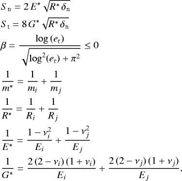 (12)
(12)
Here, E* is the effective Young’s modulus, G* the effective shear modulus, m* the effective mass, and R* the effective radius. We note that there is a mistake in the definition of G* in Di Renzo & Di Maio (2004), which was corrected in Di Renzo & Di Maio (2005).
Young’s modulus ranges from 6 to 15 GPa from 273 to 133 K for water ice (see Mellon 1997 and citations therein Gold 1958; Hobbs 1974), and for example has a value of (78 ± 19) GPa for basaltic rock mass (Schultz 1995) as proxy for our dust. However, using such high values in our simulations would require very small time-steps to resolve the Hertz collisions, and consequently very long computation times. However, Bierwisch et al. (2009) verified that E (or rather E∕(1 − ν2)) can be reduced to significantly smaller values (in the order of ≥107 Pa) without substantially affecting the simulation outcomes, and cited Martin & Bordia (2008) for the observation that a realistic value is important only if an external pressure is applied, the latter being negligible in our scenarios. We therefore take E = 108 Pa for both water ice and dust particles. For Poisson’s ratio, Schultz (1995) gave a value of 0.25 ± 0.05 for basaltic rock mass, and Mellon (1997) cited values between 0.1 and 0.3 for most rocks (Haas 1989) and around 0.4 for water ice at Martian temperatures (Hobbs 1974). We set the Poisson’s ratio for both our ice and dust particles to ν = 0.3. Finally, the coefficient of restitution generally depends on impact speed. However, since the relative velocities of neighboring particles differ only slightly, we assume er = 0.3, independent of impact speed, an intermediate value typical at normal-impact velocities of around 2 cm s−1 (Brilliantov et al. 1996). Additionally, we perform simulations with er = 0.1 and 0.8 to investigate the effect of this parameter.
Symbols.
2.2 Rolling friction
As reviewed by Ai et al. (2011), causes of rolling resistance include aspherical particle shapes, plastic deformation, viscous hysteresis, and adhesion. Ai et al. (2011) classified rolling resistance models into four different types from A to D. In Model A, a constant torque is directed against the relative rotation between two particles in contact. Although this dissipates kinetic energy, as desired, after settling of a particle assembly there remains residual energy that is dependent on the time discretization of the simulation because of a remaining torque with constant magnitude whose direction is alternating at every time-step. This can destabilize (pseudo-) static particle configurations (piles). In Model B (viscous type), rolling friction is parameterized as being proportional to angular velocity. This model properly dissipates kinetic energy, but the formation of (pseudo-) static piles requires an additional static torque. Ai et al. (2011) immediately dismissed contact-independent Model D, in which torque depends on the absolute- rather than the relative rotation or rotational velocity. This can lead to different torques being applied to each of the two particles in contact, which violates the conservation of angular momentum. Hence, we apply Model C, an elastic-plastic spring-dashpot model (EPSD). Here, the presence of both dynamic and static torques leads to kinetic energy dissipation and can support the packing structure in (pseudo-) static configurations, while it also avoids unphysical Model-A-type residual oscillations.
The equations governing Model C can be found in Ai et al. (2011, Sect. 5.3) and are here recited for later reference in Sect. 2.5. The rolling resistance torque at time t,
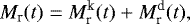 (13)
(13)
consists of a spring torque  and a viscous damping torque
  .
.
The spring torque after time increment Δt is
 (14)
(14)
with spring torque increment
 (15)
(15)
and limiting spring torque
 (16)
(16)
which is achieved at the full mobilization rolling angle  , where the particles begin to slide over each other. Here, μr is the rolling friction coefficient, and kr is the rolling stiffness, which is calculated in LIGGGHTS (DCS Computing GmbH 2016) as
 (17)
(17)
The viscous damping torque  after time increment Δt is
 (18)
(18)
in cases where  , and zero in cases of full mobilization
  , where
  is the relative rolling angular velocity between the two particles in contact. The rolling viscous damping coefficient Cr can be expressed as
 (19)
(19)
where ηr is the rolling viscous damping ratio, and Ii and Ij are the moments of inertia of the two contacting particles.
In our simulations, we have to set the rolling friction coefficient μr and rolling viscous damping ratio ηr as unitless non-negative parameters that define the magnitudes of the spring and the viscous damping torques. For numerical tests, Ai et al. (2011) used values up to 0.8 for μr and up to 1.5 for ηr, but as in translational friction, larger values are possible on physical grounds, as can be seen when considering the effective rolling friction between cog wheels for example. We use rolling friction also as a computationally inexpensive proxy for complex particle shapes.
2.3 Unsintered cohesive contacts
A particle is additionally subject to forces arising from the mere contact with or close proximity to another particle (van-der-Waals inter-particle force), which we here denote as cohesive forces from unsintered contacts. In particular, these forces do not include forces due to bonds resulting from ice sintering, and in contrast to sinter bond forces (Sect. 2.4), they do not depend on the rotational deviation from the initial state at which a contact between two particles was established.
The Johnson-Kendall-Roberts (JKR) model (Johnson et al. 1971) is widely applied to describe cohesive forces between unsintered spherical particles, but it is numerically not very efficient and also predicts significant forces even when the sphere centers are separated by distances exceeding the sum of their nominal radii, which makes it cumbersome to use in LIGGGHTS. Since the real-world cohesive forces are not exactly known for cometary particles and also depend on particle shape, roughness, cleanliness of the particles (see below), and other parameters we cannot control, we apply the numerically much simpler Derjaguin-Muller-Toporov (DMT) model (Muller et al. 1983). The DMT cohesive force,
 (20)
(20)
is independent of the Hertz-overlap, and applies as long as the spheres are nominally in contact, that is, the sphere center distance does not exceed the sum of the nominal particle radii. This force is also the value of the pull-off force defined as the force required to separate the surfaces (Barthel 2008). Here, ω is the surface energy density (or rather half the sum of the surface energy densities of the contacting partners), which is tabulated in the literature for various materials. We take ω = 0.028 J m−2 from the direct measurements by Heim et al. (1999). This value has been determined by pull-off force measurements of micron-sized silica spheres and is valid for the DMT model. Furthermore, ω for the JKR model is four-thirds of this value. We note that Heim et al. (1999) used a different definition of the surface energy density: their γ in the pull-off force − 4π R*γ corresponds to ω∕2. The different surface energy density measurements for silica spheres reviewed by Kimura et al. (2015) scatter over two orders of magnitude, with the value given by Heim et al. (1999) being more representative of the lower end. This value is compatible with recent results from Brazilian disc test measurements (Gundlach et al. 2018) that additionally suggest the surface energy density of pure water ice spheres to be similar. Since the particles present in the surface layer of comet 67P are most certainly not perfectly spherical, a reduced cohesion can be expected (Fuller & Tabor 1975; Leite et al. 2012); see below for further details.
Another approach to describe cohesion from unsintered contacts was presented by Scheeres et al. (2010), where the cohesive force for particles on asteroids is explicitly given in terms of the surface cleanliness, Sc = Ω∕tc, the ratio of the diameter of an oxygen molecule, Ω ~ 1.5 × 10⁻¹⁰ m, to the minimum inter-particle distance between two surfaces, tc. The resulting force is then estimated as  (Scheeres et al. 2010), where the proportionality factor follows from a Hamaker constant of A =4.3 × 10⁻²⁰ J and Eq. (27) by Scheeres et al. (2010),
  . The motivation of a formulation in terms of the surface cleanliness is given by the fact that two surfaces cannot come in close contact in terrestrialenvironments, because they are contaminated by atmospheric gas molecules. This leads to a decrease in the attractive force (Sc ~ 0.1). In space environments, the contamination is smaller, and stronger forces can be expected (Sc → 1). Scheeres et al. (2010) also recited results by Castellanos (2005), who experimentally investigated the effect of surface asperities of particles with typical asperity radius Ra, where Ra < R. In this case, or when the particles are covered by smaller particles of radius Ra, the forces scale with Ra instead of R*, i.e., Fc,a ~ Fc Ra∕R* (Scheeres et al. 2010). Comparing with the plain DMT cohesive force, one can write
  , which translates to Sc = 1.56, and on the other hand we have
  .
.
In conclusion, for the cohesive forces from unsintered contacts we apply DMT theory with ω from Heim et al. (1999), but regard this as an upper limit. For complex-shaped particles, we assume Ra ∕R* to be on the order of 0.1–1.0. In our simulations, we therefore have to also investigate the effect of the DMT cohesive force being reduced by a certain factor; see also discussion in Sect. 4.1. Finally, Scheeres et al. (2010) investigated the relative importance of the physical forces acting on particles on the surface of small Solar System bodies. Applying the findings of these latter authors to the situation in our 67P simulation scenarios, self-gravity, solar radiation pressure, and electrostatic forces away from the terminator can be neglected compared to cohesive forces from unsintered contacts and to ambient surface acceleration.
2.4 Parallel bonds
As reviewed by Blackford (2007), when particles containing water ice are in contact over longer time-spans, they sinter, that is, necks form between them that grow with time, resulting in rigid bonds. This is even the case in the absence of pressure or melting, and can also take place without water vapor transport simply by surface or volume diffusion of water-ice molecules in the solid material. Water-ice sintering is only efficient when the absolute temperature is warmer than about 60% of the melting point (Blackford 2007, Fig. 11; reprinted from Maeno & Ebinuma 1983). The dominant processes are surface diffusion and vapor transport, the former being more efficient for colder temperatures and small sinter necks (Blackford 2007, Fig. 10; reprinted from Maeno & Ebinuma 1983). Regarding the diurnal and seasonal illumination cycles and the heat diffusion from the illuminated surface into deeper layers, the maximum sintering rate occurs at the surface down to a few thermal skin depths, where the ice experiences the highest temperatures (Molaro et al. 2019). In the case of 67P, we therefore expect the most and strongest sinter bonds to occur within the topmost layer on the scale of centimeters (diurnal) to meters (seasonal), considering the thermal inertia of about 10–50 J K−1 m−2 s−1∕2 inferred from measurements of the MIRO instrument aboard Rosetta (Gulkis et al. 2015). However, in the uppermost layers, sublimation of volatiles is also efficient leading to desiccation and thus fewer or weaker sinter bonds, at least partly balanced by recondensation during night, all of which potentially leads to a complex sinter bond and strength pattern with depth.
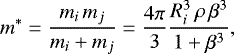
We apply the parallel bonds model by Potyondy & Cundall (2004) in our DEM framework to simulate the inter-particle forces resulting from such sinter bonds. Our implementation is based on the LIGGGHTS-WITH-BONDS package (Richter 2015), which is a beta version aimed at implementing the cited parallel bonds model. Such bonds are initially formed in the simulation when the surfaces of two particles are closer than a fraction of their mean radius and break when the inter-particle stresses exceed certain threshold values. We do not switch off the cohesive forces from the unsintered contacts when a sinter bond is formed because for a very weak sinter bond for example (immediately after its initial formation in case of real material) this would otherwise actually lead to an abrupt decrease of the inter-particle force, which we judge to be unrealistic and which is numerically unstable. In the other extreme, in case of a very strong sinter bond, a numerically still active cohesive force due to unsintered contacts does not significantly affect the result and incurs only minor computational overheads. Once broken, we do not let a sinter bond form again because the timescale for sintering is assumed to far exceed the simulated time-span. Potyondy & Cundall (2004) pointed out that on the microscopic level, parallel bonds exclusively break in case of tension between particles, not in case of compression. Macroscopic compressional fracturing of the material is caused by bond breakage due to lateral tension between particles resulting from the macroscopic compression. We note that LIGGGHTS-WITH-BONDS has to be modified in this regard to correctly implement Eq. (16.1) from Potyondy & Cundall (2004).
Potyondy & Cundall (2004) regarded a parallel bond between two bonding partners as a beam in classical theory of elasticity. The bond cement has mechanical properties that we take – in the absence of more detailed knowledge – to coincide with those of the bonded spheres themselves (motivated by the sintering being a result of the redistribution of the sphere material; at least of the water-ice part of it). In particular, this applies to Young’s modulus  and Poisson’s ratio
  , where the overlines indicate parameters of the bond cement as opposed to parameters of the spheres. Following Silbert et al. (2001), we set the ratio between normal and shear stiffness
  . Additional bond properties include the bond radius
  , with the radii Ri and Rj of the bonded spheres and parameter
  scaling the bond radius, and the tensile and shear strengths of the bond cement,
  and
and  , respectively. To reduce the parameter space, we take
  and verified that the choice
  leads to very similar simulation outcomes, which is related to the observation that most bonds in our simulations break due to normal stress. Assuming a bond state intermediate between barely (
 ) and completely sintered (
 ), we set
  . Mellon (1997) recited values of
  between 1 and 2 MPa for water ice, and a moderately wider range for polycrystalline ice samples or frozen soils, all depending on strain rate, temperature, and sample size. Given the uncertainties, we use a reasonable generic value of
  Pa.
Pa.
The force  and moment
  carried by the parallel bond are computed as the sums of their normal (n) and tangential (t) components with respect to the contact plane,
 (21)
(21)
which are initialized to zero at bond formation and are then integrated from their increments
 (22)
(22)
Here, ΔUn is the increment of the sphere overlap taking into account changes in both sphere center positions and sphere radii, and ΔUt is the increment of the tangential displacement taking into account both rotation and sphere center positions. Δθn and Δθt are the relative rotational increments of twisting and bending. The tangential components in Eq. (22) have to be rotated before summation to account for orientation changes of the contact plane.  ,
,  , and
, and  are the area, moment of inertia, and polar moment of inertia of the parallel bond cross-section, respectively. For cylindrical bonds with radius
  , these quantities are
  ,
,  , and
, and  .
.
Motivated by classical beam theory, Potyondy & Cundall (2004, Eq. (18)) defined
 (23)
(23)
With these definitions, the particle size dependence of the macroscopic elastic properties of an example material was demonstrated by these latter authors in several 3D simulations to become only minor. For each of our simulation scenarios that involves parallel bonds, we exemplarily check the influence of the particle size (or rather of the coarse-graining factor discussed in Sect. 2.5) on the macroscopic behavior.
A parallel bond breaks when the maximum tensile stress  acting on the beam-analog of the bond exceeds the bond’s tensile strength
  , or when the maximum shear stress
  exceeds the bond’s shearstrength
  , where, according to Potyondy & Cundall (2004, Eq. (16)),
 (24)
(24)
2.5 Particle sizes and coarse-graining
The particle sizes affect the interparticle forces. For instance, the DMT cohesive force (Eq. (20)) increases linearly with particle size (Muller et al. 1983). In the same way, forces due to sinter bonds in the model of Potyondy & Cundall (2004) depend on the radius of the smallest particle of the bond pair. In case of monodisperse spheres, the interparticle forces are degenerated, causing objects made of such particles to disintegrate quite homogeneously around a specific macroscopic force threshold. For example, a dropped boulder either completely disintegrates or remains undamaged, with a very narrow transition range and depending on the external forces acting on the body. To achieve a more realistic behavior, with only parts of the object disintegrating, polydisperse particles are used in our models. Using just two or three different particle radii still leads to a bond force degeneration, since it is quite likely that at least one of the two bonded partners is of the typically more frequent small size resulting in a degeneration of bond radius  . Because of the way types of particles and their properties are implemented in LIGGGHTS, we cannot use a continuous size distribution without larger code changes. Therefore, we use a discrete particle size distribution with eight different equally spaced radii, but the impact of using more bins is tested as well. We note that due to modeling complexity and the limited available computational resources, we do not investigate the presence of small interstitial particles partially filling the voids between the larger particles and their potential cohesive effects.
The cumulative particle size distribution is set to follow a power-law with index ic such that the number of particles with radius larger than R is proportional to R−ic. Mottola et al. (2015) reported ROLIS measurements for Agilkia, the initial touchdown site of the Philae lander, exhibiting values of ic in the range from 2.2 to 3.5. We note that the exponent of the corresponding differential size distribution is ic +1, and that of the incremental size distribution with logarithmic radius increments is ic (Colwell 1993). Here, ic = 2 translates to a uniform mass distribution with respect to particle radius. Since the number of particles in a DEM simulation is limited by the available computational resources, with our scenarios typically comprising on the order of 104 –106 particles, the minimum particle size is limited by the volume that needs to be filled. Similarly, the maximum particle size is limited by the spatial extent of the simulation domain, but typically we use a much smaller maximum particle size than that because the steep particle size distribution requires a low ratio between the radii of the largest and the smallest particles to ensure a statistically representative number of large particles. In our simulations, we use ic = 2.5, and the ratio between the radii of the largest and the smallest particle is 2, meaning that eight of the smallest particles have the same mass as one of the largest ones.
Our simulation scenarios have typical dimensions of 1–100 m, often leading to a prohibitively large number of particles when we assume particle radii in the reasonable range of millimeters to centimeters. This is why we apply the coarse-graining scheme of Bierwisch et al. (2009), where instead of the physical particles, an effective medium of computational parcels is considered, each parcel representing groups of several particles. The coarse-graining factor cg scales the radius of the computational parcels relative to the radius of the original particles. Bierwisch et al. (2009) argued that in order to obtain simulation results that are statistically similar between the scaled and the unscaled system, the model parameters of the computational parcels have to be scaled in such a way that the energy density and evolution of energy density are the same as for the unscaled system. Applying coarse-graining, we can save computational resources by reducing the number of particles that have to be considered, enabling the simulation of macroscopic scenarios with small particles. In addition, we can better manage different size scales of the respective scenarios when comparing mechanical parameters between them.
We now investigate the scaling of the volume densities of gravitational potential energy, potential energy in unsintered and sintered cohesive contacts, and translational and rotational kinetic energy, all with respect to the coarse-graining factor cg. In the following, scaled quantities are indicated by a prime, and the unscaled ones are written without prime. The radius of a computational parcel is scaled as R′ = cg R.
Consider N spherical particles with solid mass density ρ, radii Ri, and masses  experiencing ambient surface acceleration g in a volume V. Additionally, we assume that the considered volume is sufficiently small that kinematic quantities such as particle speed vi = |vi| and vertical position zi are approximately the same (v and z) for all particles in this volume. Following the arguments of Bierwisch et al. (2009), the density of the gravitational potential energy U,
 (25)
(25)
where the sum is taken over all particles in the volume V, is independent of cg when the solid mass density ρ and the filling factor  are constant, i.e. ρ′ = ρ and ϕ′ = ϕ. This means that, when leaving ρ constant, we have to ensure that ϕ is unaffected by the scaling, which is the case when we leave the particle size distribution normalized with respect to the minimum particle radius unchanged.
The density of the translational kinetic energy K reads
 (26)
(26)
where, because the solid mass density and the filling factor are constant, we have to ensure that the velocities are unaffected by the scaling. Then, gain and loss of kinetic energy are given by the surface acceleration, which is independent of particle size, and by collisionsbetween particles governed by the Hertz contact law. For two contacting particles, Eq. (5a) can be written as
 (27)
(27)
where β = Rj∕Ri is the ratio of the radii of the colliding particles. Inserting Eq. (28) into Eq. (27) and using dimensionless variables  and t† = t v0∕Ri with a reference velocity v0, Eq. (27) reads
 (29)
(29)
A dimensional analysis shows that the velocities are independent of cg when β is constant, i.e. β′ = β, and when  and
and  . This scaling is already fulfilled by way of Eqs. (11) and (12) when leaving Young’s modulus constant, i.e. E′ = E. Similar scaling considerations for the density of the rotational kinetic energy show that the tangential coefficients kt and γt as defined by Eq. (11) do not need to be additionally scaled either.
The cohesive potential energy density in the DMT model, using Eq. (20), reads
 (30)
(30)
with the effective radius
 (31)
(31)
and where the sum is taken over all contact partner pairs in the volume V. Here, we exploit the fact that the parcel number in the volume V scales with cg−3, when the particle size distribution normalized with respect to the minimum particle radius is unchanged. Since β is constant, the DMT cohesive potential energy density is independent of cg when ω′ = cg ω.
A dimensional analysis of Eqs. (16)–(19) shows that the rolling friction coefficient μr and rolling viscous damping ratio ηr are not scaled with cg.
Similarly, the potential energy density of a sinter bond, using Eqs. (22) and (23),
![\begin{eqnarray*} \frac{\sum_i \Delta\overline{F}_{\textrm{n}}\,\Delta U_{\textrm{n}}}{V}&=&\frac{\sum_i\overline{k}_{\textrm{n}}\, \overline{A}\, \Delta U_{\textrm{n}}^2}{V}=\frac{\sum_i\frac{\overline{E}}{R_i+R_j}\, \pi\overline{R}^2\, \Delta U_{\textrm{n}}^2}{V} \nonumber\\ &&\sim\frac{\left[\min(1,\beta)\right]^2}{1+\beta}\frac{\overline{E}\,\Delta U_{\textrm{n}}^2}{R_i^2}, \end{eqnarray*}](/articles/aa/full_html/2020/09/aa37152-19/aa37152-19-eq77.png) (32)
(32)
is independent of cg when the Young’s modulus  of the bond cement is constant, i.e.
  , because β is constant and both the increment of the sphere overlap ΔUn and the parcel radius Ri scale with cg. In addition, Eqs. (24) imply that
  and
and  do not scale with cg, which is why the tensile and shear strengths of sinter bond,
  and
and  , respectively, are also not scaled. In other words, the definition of
  and
and  according to Eqs. (23), intended by Potyondy & Cundall (2004) to minimize the particle size dependence of the macroscopic elastic properties, ensures that our simulations become almost statistically independent of cg.
In conclusion, velocities scale with cg0, parcel radii with cg1, forces with cg2, and torques with cg3. Moreover, we deduce that the time-steps in the simulation scale with cg. This implies that for a given simulation volume to be filled with computational parcels, and for a given span of real time, the required computer memory scales with cg−3, whereas the processing time scales with cg−4. All the scalings are automatically fulfilled by the parameter definitions recited in Sects. 2.1–2.4, once parcel radii and the surface energy density ω are scaled with cg, and for numerical efficiency, the time-steps can also be scaled with cg, whereas the cutoff distance for building the neighbor lists (see Sect. 2.1) has to be scaled with cg for numerical stability. No other of the remaining physical parameters that we have to set in our DEM simulations (ρ, ϕ, g,  ,
,  , er, μ, μr, ηr,
  ,
,  ,
,  , ic) is scaled with cg.
We would like to point out that these are only first-order scaling rules, and in practice, corrections may be necessary toachieve a comparable morphologic behavior between the scaled and the unscaled system. In particular, working with a certain size distribution for computational parcels does not mean that the physical particles follow this size distribution. Also, this approach neglects interparticle collisions and energy and momentum dissipation within a given computational parcel; see Radl et al. (2011) for comparison. Therefore, we always exemplarily check whether the morphologic features of the simulation results are indeed mostly unaffected when cg is varied within a reasonable range. In cases where it is not possible due to insufficient computational resources to compare to full-resolution results, we compare results for different coarse-graining factors as widely separated as half an order of magnitude. Depending on particle size and the scenario dimensions, we use coarse-graining factors typically on the order of 1–100. For convenience,we use the terms “particle” and “parcel” interchangeably in the following when referring to simulations. Indeed, all our simulations are performed with parcels, even when coarse-graining is switched off, which is accomplished by setting cg = 1. Physical 67P particles are explicitly referred to as “particles”.
3 Simulation scenarios
We consider two different simulation scenarios that are related to observations on comet 67P by Rosetta: the stability of boulders and the collapse of cliffs. A third scenario serves to estimate the tensile strength for our model materials for direct comparison to estimates derived from Rosetta measurements. The simulation outcomes are presented and discussed in Sect. 4.
3.1 Boulder stability
We start with the requirement that boulders of sizes observed on the nucleus surface have to be stable without collapsing under their own weight or when falling from smaller (e.g. during cliff collapses) or greater (from the coma) heights. For this purpose, we assume a large spherical boulder to be made up of small particles and investigate conditions for it to be reasonably stable when being dropped from small altitudes above a hard surface.
Our boulders are 2 m in diameter and made up of a mixture of two types of particles that consist of different materials: either dust or water ice. For simplicity, the particle types are assumed to differ only in their mass density (dust: 2000 kg m−3, ice: 920 kg m−3) and their ability to form bonds from sintering (dust–dust: no bonds, ice–dust: no bonds, ice–ice: bonds) as the conditions on the comet allow only the sintering of ice. In particular, it is assumed that both particle types have the same size distribution, mechanical parameters, and surface energy density of unsintered cohesive contacts. The latter assumption is motivated by recent laboratory experiments with dust and ice particles at low temperatures (Gundlach et al. 2018). We simulate boulders made up of pure dust and of two dust-ice mixtures with a dust-to-ice volume ratio (ice volume fraction) of 2:1 (33%), and 1:1 (50%), respectively. The macroscopic porosity of the material is prepared between 63 and 73% depending on the ice content in order to achieve a bulk density of the boulder that is similar to the global mean value of 538 kg m−3 for comet 67P (Preusker et al. 2017).
As a typical impact velocity of the boulder, we take the free-fall velocity from 30 m above the surface, which is about 0.1 m s−1 for a typical surface acceleration on 67P of 1.8 × 10⁻⁴ m s−2 calculated as the median over all facets of the 67P shape model (Preusker et al. 2017). We simulated vertical impacts as well as oblique impacts with an impact angle of 30° (measured from the normal to the surface). Since we did not observe major morphological differences between results for these impact conditions, we only show oblique impacts as they lead to a better visual separation of the post-impact boulder fragments than vertical impacts.
The simulation is composed of two parts – the construction of the spherical boulder, and its impact on the surface. It starts by loosely filling a large sphere with noncontacting randomly sized and positioned particles. This particle cloud is then compacted to the desired level by equally accelerating all particles in the direction of the particles’ center of mass. As the particles converge towards this point, they collide with each other and dissipate their kinetic energy. By changing the particles’ initial velocity and (temporarily) the interparticle contact parameters, we can control the bulk mass density and porosity of the emerging boulder. After settling, excess particles outside the intended boulder diameter are removed, and contacting particles capable of sintering are bonded. Settling of the particles is ensured after every preparation step, and we verify that the prescribed size distribution, mixing ratio, porosity, bulk mass density, and homogeneity have indeed been achieved after the preparation phase. The boulder is then moved to a position directly above the surface and instantaneously accelerated to its impact velocity by setting the velocity of all particles to that value. The simulation is run until the boulder or its fragments have settled afterthe primary impact. An example of the boulder stability scenario is shown in Fig. 2.
This simple scenario is suited to study the effects of changing the material composition (ice content) of the boulder and the particle properties including size distribution, mechanical parameters, surface energy density, and so on, which is information that can be used for setting up the more complex cliff collapse scenario (Sect. 3.2).
3.2 Cliff collapse
Cliff and overhang collapses have been observed on 67P, and their debris is abundant on the nucleus surface (Pajola et al. 2017; Vincent et al. 2016; Groussin et al. 2015). We develop a corresponding simulation setup starting with the results from the boulder stability scenario (Sect. 3.1).
Motivated by a survey of 20 overhanging cliffs on 67P in Attree et al. (2018), our cliff is set to be 30 m high and has an overhang with an angle of 10°, 20°, or 30°, respectively.The material is a mixture of dust and ice particles identical to the material used for the boulders. It is assumed that the collapse is made possible by a weakness in the cliff material that cannot withstand significantly more stress than the pressure exerted by 67P’s surface acceleration. This weakness could result from natural variations in the material composition or from structural defects, in particular cracks caused for example by thermal fracturing or by material loss or sinter bond annihilation due to sublimation. The collapse of a barely stable cliff could then be triggered by the crack expanding beyond a critical threshold, or by low seismic activity, for example due to impacts (Richardson et al. 2005) of small interplanetary meteoroids or of boulders falling from the coma, or due to tidal and self-gravity stresses of the nonspherical nucleus and stresses induced by changes of the rotation period of the comet due to nongravitational forces (Hviid et al. 2016; Matonti et al. 2019).
The simulation starts by inserting noncontacting randomly sized and positioned particles with a given downward velocity above a cliff-shaped region confined by walls. As the particles fall down, they gradually fill the space between the cliff walls from the bottom to the top. By changing the insertion velocity and (temporarily) the interparticle contact parameters, we can control the bulk mass density and porosity of the emerging cliff. After settling, excess particles beyond the given cliff height are removed, and particles capable of sintering are bonded, but only in the top layer (3 m) to account for the fact that sintering is most efficient near the surface (see Sect. 2.4). Finally, the wall supporting the overhang is removed and the collapse of the cliff is triggered. The simulation is run until the particles forming the debris pile have settled. An example of the cliff collapse scenario is shown in Fig. 3.
Seismic shaking as the collapse trigger is implemented by moving the remaining walls (bottom, back, and sides) along the main coordinate directions with velocities that follow sine functions with certain frequencies, amplitudes, and phases that differ between the directions. These vibrations are transferred by the wall–particle forces to the particles in direct contact with the walls and from there travel further into the cliff material. High frequencies are dissipated more efficiently than lower ones, while overly low frequencies do not lead to significant stresses in the cliff material. Hence, a certain intermediate frequency range is the most effective as a collapse trigger. Regarding the vibration amplitudes, overly small values have no effect, whereas very large ones completely disintegrate the cliff in an unrealistic way, necessitating a balanced choice as for the frequencies.
The pre-collapse dimensions of the cliff, considering it has to support itself before initiating the collapse trigger, and the post-collapse boulder size distribution and angle of repose can provide us with constraints on mechanical parameters. This scenario also permits the study of collapse triggers.
 |
Fig. 2 Construction and simulated drop of a sintered two-meter-sized boulder made up of a 2:1 dust–ice mixture (34 000 computational parcels) from 30 m above the surface (beige-colored plane) of comet 67P. Oblique impact with impact speed of 0.1 m s−1 and impact angle of 30° measured from the normal to the surface. Top row: construction of the boulder. (a) Loose filling of a large sphere with noncontacting randomly sized and positioned dust (gray spheres) and ice (blue spheres) particles. (b) Compaction of the boulder to the bulk mass density and porosity of comet 67P. (c) Removal of particles outside the intended boulder diameter and formation of sinter bonds (thick red bars) between ice particles. Bottom row: (d–f) Several stages after impacting the surface of 67P; sinter bond representation is omitted for clarity. Lighter shades of gray or blue visualize a higher topography. In case (c), the material is visualized partly transparent. |
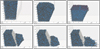 |
Fig. 3 Construction and simulated collapse of a 30-m-high cliff made up of a 2:1 dust–ice mixture (65 000 computational parcels) with a sintered top layer of 3 m thickness. Top row: construction of the cliff. (a) Loose filling of a region confined by walls with noncontacting randomly sized and positioned dust (gray spheres) and ice (blue spheres) particles. (b) Compactionof the cliff to the bulk mass density and porosity of comet 67P. (c) Removal of particles beyond the given cliff height, formation of sinter bonds (thick red bars) between ice particles in the top layer of the cliff, and removal of the wall supporting the overhang. Bottom row: (d–f) Several stages after triggering the collapse. Representation as in Fig. 2. Particles in white are from the initial crack region. |
3.3 Tensile strength test
This additional scenario serves to estimate the tensile strength for our model materials for direct comparison to estimates derived from Rosetta measurements. The microscopic parameters (particle size distribution and geometrical configuration, surface energy density, friction coefficients, etc.) manifest in a macroscopic strength of the material. To determine the strength of our model materials, we perform a numerical simulation of a tensile strength test, where an elongated material sample is pulled to its breaking point. In our test, we prepare a cylinder of 5 cm (diameter) × 10 cm (height) in dimension consisting of a sufficient number of small particles to avoid significant boundary effects. This is mounted in a clamp (a wall with the shape of a truncated cone) with its flat top side, while a gradually increasing force is pulling on the flat bottom side of the cyclinder. We monitor the forces experienced by the clamp. Mediated by the cylinder material, the force registered at the clamp corresponds to the one applied at the bottom. It increases as long as the cylinder is intact, but rapidly decreases as soon as the cylinder breaks apart. The force at the breaking point normalized over the cylinder’s cross-sectional area is defined as the material’s tensile strength, which we can calculate from our model readings in order to compare it to the values of the real cometary material recited in Sect. 1 and to laboratory measurements of cometary analog materials.
4 Results and discussion
In this section we report and discuss the outcomes of our simulations for the basic scenarios, and the changes that occur when modifying the setup or varying the parameters.
4.1 Boulder stability
Before starting the actual dropping simulations, we investigated boulders resting on the surface and found them to be stable (except for small deformations around the contact at the bottom) up to diameters exceeding that of the largest boulders observed on the surface of 67P (~50 m).
For each material composition, we then simulated drops of boulders made up of particles respecting the relative size distribution from Sect. 2.5 scaled to cover six different diameter ranges: 0.2–0.4 mm, 0.4–0.8 mm, 1–2 mm, 2–4 mm, 4–8 mm, and 10–20 mm, in total covering about two orders of magnitude, with a corresponding opposite effect on stability. For each case, we performed simulations with three distinct levels of friction: one with low to medium friction (triple of friction coefficients μ∕μr∕ηr of 0.8∕0.2∕0.3, adopted from Ai et al. 2011), one with high friction (coefficients 1.0∕1.0∕1.0), and one with very high friction (coefficients 2.0∕2.0∕2.0). High friction levels can be used as a proxy to describe interlocking between complex-shaped particles. For the dust–ice mixtures, we performed all simulations twice, either with or without sintering of the ice particles. In total, and with additionally probing the influenceof other parameters, such as for example the boulder size and impact conditions, we performed over 100 different boulder drops each made up of 30 000–40 000 computational parcels and always taking about 200 CPU-core hours of processing time. As we cannot show all of them here, we have selected a limited set that still captures themain effects of changing the various model parameters. Figure 4 shows the influence of friction and particle size for boulders made of pure dust, and Figs. 5 and 6 show the effect of friction, ice sintering, and particle size for boulders made of the 2:1 and the 1:1 dust-to-ice mixture, respectively.
We exemplarily investigated moderate changes in the coarse-graining factor cg (increase by up to half an order of magnitude compared to our respective highest-resolution level). While the details of, for instance, the fragmentation (location and shape of cracks, exact number of fragments, spatial arrangement of debris pile) can be quite different, the general trend in the morphologic behavior (complete disintegration, breakage into large/small fragments, undamaged)and observables like settling time, extent of debris field, or macroscopic pressure at impact point are largely preserved. Since the precise geometric arrangement of the computational parcels slightly changes with cg, the simulation outcomes have to be interpreted within tolerances given by slight changes in the geometric arrangements at unchanged cg. This can give rise to a behavior of deterministic chaos. Starting for example with a different realization of the random parcel initialization, the parcel that first contacts the bottom plane is different, as is the configuration of its neighbors, which can lead to a different simulation outcome, a situation reminiscent of the nonlinear properties of the real particle ensemble. However, we have to avoid overly coarse resolutions to keep the fraction of parcels that are at the boundaries of the boulder or its fragments low. At extremely low resolution, where almost all parcels are at or close to the boundaries, the simulation outcome is completely meaningless.
When impacting the surface, the boulder has to withstand the forces arising in the collision as well as the surface acceleration of the nucleus. In general, the boulder remains undamaged after impact when the interparticle forces (from unsintered and sintered cohesive contacts) are set too strong, whereas it totally disintegrates upon impact when they are set too weak. A reasonable behavior somewhere in between would cause the boulder to break up into large fragments with some debris, or lead to partial damage of the main body with some smaller parts broken off.
Without sinter bonds
When the simulation is run without sinter bonds between the ice particles, the boulder is held together by cohesive forces from unsintered contacts only. This simpler case is suited to studying the effects of changing the particle size distribution and the mechanical properties of the particles separately from the properties of the sinter bonds.
The inability of the ice particles to form sinter bonds implies that the only remaining difference between both particle types is their mass density, and varying the ice content of the material requires a change of porosity to maintain the desired bulk density of the boulder of about 0.53 g cm−3. For our twolimiting cases of pure dust and the 1:1 dust–ice mixture, with a solid mass density of 2000 kg m−3 and 1460 kg m−3, the required porosity of the material is 73 and 63%, respectively. The larger filling factor of the ice-rich boulder means that the particles aremore closely packed and on average in contact with more neighboring particles. For our porous materials, a particle typically adjoins only two or three neighbors, corresponding to a mean coordination number between 2.1 for pure dust and 2.9 for the 1:1 dust–ice mixture. This translates to a higher strength of the ice-rich boulder, but this effect is generally small, and, compared to other factors influencing the boulder’s stability, it is too small to constrain the ice content of the material by matching the simulation outcomes to the observed morphologies, all other parameters equal.
A larger, clearly noticeable effect on the stability of the boulders is observed when changing the particle size distribution. In general, objects made up of larger spherical particles are less stable. More precisely, the strength of the material scales inversely with particle size (∝R−1), because thenumber of contacts between two particle layers scales with R−2, while the DMT cohesive force of a single contact scales with R (Eq. (20)). This means that increasing the particle size by one order of magnitude decreases the strength of the boulder by a factor of ten. An equivalent effect can be produced by leaving the sizes but assuming the particles have surface asperities with typical asperity radii Ra of one tenth of the sphere radii (see Sect. 2.3).
As discussed above, we are restricted to a limited particle size range in our simulations, with the ratio between the radii of the largest and the smallest particle being generally set to two. We found that when doubling the largest particle radius while keeping the smallest one, the size distribution index, and the bin size (thus using 22 size bins), the material strength decreases (morphologically comparable to the case with a ratio of two with all radii multiplied by a factor in the order of 1.5) in our boulder stability scenario (1:1 dust-to-ice ratio, high friction, no sintering). This suggests that, even though the material becomes stronger when extending the size range towards smaller particles, there is a certain effective particle radius between the smallest and the largest radii around which the size range can be (in a suitable and moderate way) extended without major morphological impact: The increased strength from adding smaller particles is compensated by adding larger particles.
Using an additional simulation, we verified that the relatively small number of eight particle size bins we generally use in the present paper is not critical to our results. Keeping the largest and the smallest particle size and the size distribution index but utilizing 22 instead of eight bins yielded morphologically equivalent simulation outcomes. In the same way, a smaller time-step of 3% instead of 10% of the minimum of Rayleigh time and Hertz time resulted in morphological equivalence as well as unchanged settling time.
In addition to our reference value of 0.3 for the coefficient of restitution er, we also performed simulations with er set to 0.1 and 0.8, respectively, to investigate the sensitivity to this parameter. Higher coefficients of restitution led to a larger amount of small debris but only moderate morphological changes to the large fragments. Additionally, all fragments were distributed over a larger surface area. Similarly, an additional simulation with a Young’s modulus of 1 GPa, which is ten times the nominal value in our other simulations, had a longer settling time and showed a higher degree of fragmentation, corresponding to a lower level of internal energy dissipation. In both of these cases, the resulting morphology was similar to that associated with boulder drops from higher altitudes or boulders made up of constituents that have a Young’s modulus of 0.1 GPa but are twice as large.
Our simulations show that boulders made up of sub- millimeter-sized or smaller particles remain more or less undamaged after impact, while boulders made up of centimeter-sized or larger particles totally disintegrate upon impact. We note that some boulders on 67P have been observed to be particularly stable; it is believed that some have even bounced over the surface several times before finally coming to a rest (Vincent et al. 2019). Boulders made up of millimeter-sized particles show a plausible behavior that is somewhere between the no-damage and the total-disintegration cases. At the lower end of this size range, the boulder is deformed from its initially spherical shape into an oblate shape with only small amounts of material being broken off. For gradually larger constituents, the boulder can break apart into several large fragments, or an increasingly larger fraction of material is broken off and dispersed into gradually smaller fragments over a larger area, forming a debris field. This debris field is relatively flat and resembles a continuous layer of similarly sized small boulder fragments. We attribute this lack of larger fragments in the debris field to the structural homogeneity of the boulder in the absence of sinter bonds. When the index ic of the power-law is set to a larger (steeper) value, the number of smaller particles is increased with respect to the number of larger ones, which translates to a higher strength and thus to more stability.
Translational friction and rolling friction also hamper the boulder’s deformation and disintegration, but their effect on the stability of the boulder is smaller than that of the particle size distribution. More importantly, friction affects the elasticity of the boulder and the roughness of the post-impact morphology. Low friction leads to a weaker and more elastic boulder that is easier to deform and features a smoother post-impact morphology. High friction leads to a stronger but more brittle boulder that is harder to deform, but if it is deformed, it “breaks” and features a sharper-edged post-impact morphology.
Finally, we investigated the behavior when the properties of the bottom surface impacted by the boulder are moderately altered. We find that a very dissipative surface (e.g., some tough material covered with a layer of finer debris) with a restitution coefficient of 0.1 instead of our reference value 0.3 does not lead to significant morphological changes. The same applies for the Young’s modulus of the bottom surface decreased by one order of magnitude (i.e., E = 107 Pa).
Our results suggest that the constituents of the cometary surface material, if spherical, have diameters mostly on the order of 10−3 m for a surface energy density of ω = 0.028 J m−2. For a lower or higher surface energy density, the constituent sizes of stable boulders have to be scaled by the same factor to maintain the strength of the boulder and observe the same post-impact morphology as before. The breaking of boulders into large fragments requires high levels of friction, which suggests that cometary particles are probably not all spherical but at least partly highly angular or very rough. This also translates to weaker interparticle cohesive forces (asperity effect, Sect. 2.3), which has to be compensated by a correspondingly smaller particle size to again arrive at the same morphology. These observations can be carried over when heterogeneities are allowed by introducing locally more stable regions (e.g., smaller or less rough particles, higher coordination number).
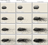 |
Fig. 4 Post-impact morphology of dropped two-meter-sized boulders made up of dust particles from different size ranges (rows). Impact conditions and graphical representation as in Fig. 2, but the indication of the particle type (water ice vs. dust) by colors is omitted for clarity here and in the following. Left column: low friction. Mid column: high friction. Right column: very high friction. |
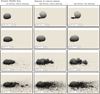 |
Fig. 5 Post-impact morphology of dropped two-meter-sized boulders made up of a 2:1 dust–ice mixture of particles from different size ranges (rows) and under different friction and sintering conditions (columns). Impact conditions and graphical representation as in Fig. 4. |
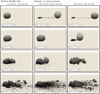 |
Fig. 6 Post-impact morphology of dropped two-meter-sized boulders made up of a 1:1 dust–ice mixture of particles from different size ranges (rows) and under different friction and sintering conditions (columns). Impact conditions and graphical representation as in Fig. 4. |
With sinter bonds
In this case, ice particles can form sinter bonds between each other, which hold the boulder together in addition to cohesive forces from unsintered contacts, and whose number depends on the ice content of the material. This more complicated case is therefore suited to studying the effect of the ice content and the sinter bond properties.
We can measure the number of broken sinter bonds referred to the number of intact ones before impact. A morphologically reasonable behavior is associated to a sinter-bond-break ratio on the order of typically 10 to 50%. Total disintegration (100%) and total stability (0%) may both occur in reality on the nucleus due to local variations in the material of the comet. However, here we focus on cases with partial damage because they are subprocesses of larger scenarios, in particular of cliff collapses (Sect. 4.2), which is why we take the 30-m-free-fall velocity as reference for the boulder stability scenario.
To estimate the influence of ice sintering on the dust–ice mixtures used in our simulations, we calculate the fraction of sintered contacts when the ice particles are distributed homogeneously in the boulder. This number does not scale linearly with the ice content as a higher ice content reduces the average distance between two ice particles and thus increases the probability of ice particles being in contact with each other, in addition to the higher number of ice particles in general. For an ice volume fraction x = Vice∕V ≈ Nice∕N and a coordination number CN, an ice particle is on average in contact with x ⋅ CN other ice particles. This results in a total of x ⋅ CN ⋅ Nice∕2 (division by two to not count contacts twice) sinter bonds in addition to a total of CN ⋅ N∕2 unsintered cohesive contacts in the boulder (we reiterate that we do not switch off cohesion from unsintered contacts when a sinter bond is formed). The fraction of contacts that are additionally sintered is therefore x2. For our dust-to-ice volume ratios (ice volume fraction) of 2:1 (33%) and 1:1 (50%), this gives a fraction of 11% and 25% of sintered contacts, respectively, suggesting a rapidly decreasing influence of ice sintering for increasingly ice-poor materials.
Our simulations confirm a relatively small influence of ice sintering for homogeneous boulders with a dust-to-ice volume ratio higher than 2:1. The bond network of sintered ice particles can be pictured as a skeleton with other particles attached to it. For a lower ice content, this structure is more fragile as individual clusters of ice particles in the boulder are connected by just a few easily breakable sinter bonds (in addition to the unsintered background), or not connected at all. For a 1:1 dust-to-ice volume ratio, the debris fields of dropped sintered boulders show a strong clustering of ice particles compared to the homogeneous and flat debris fields of unsintered boulders. In addition, and similar to the effect of high friction, a sintered boulder is more rigid and more brittle; it deforms less, but if it does, it rather “breaks” into more fragments that are clearly distinguishable.
Using an additional simulation, we investigated the effect of bulk mass density and porosity on the stability of sintered boulders. In this simulation, we prepared a material with a larger bulk mass density of about 800 kg m−3, which corresponds to a lower porosity of about 45% for our 1:1 dust-to-ice mixture. As expected, the sintered, less-porous boulder was noticeably stronger and more brittle, which can be attributed to the higher coordination number of the particles resulting in a larger number of bonds.
Both friction and sintering have the effect of increasing the strength and the brittleness of the material. However, if no debris field is present after the impact, the post-impact morphologies can be quite similar and difficult to distinguish from one another. If a debris field is present, the effects of high friction, and of additional sinter bonds and low friction, can be clearly distinguished based on the clustering of the debris. For a 2:1 dust-to-ice volume ratio, the influence of sintering is noticeably weaker but still recognizable. For even higher dust-to-ice volume ratios, the influence of sintering is too small to reliably distinguish between a sintered andan unsintered boulder solely based on morphology. On the basis of the clustering in the debris fields and the angularity of boulders imaged on the surface of 67P, our numerical results again suggest that the friction coefficients of the surface material can be comparatively high in places, and additionally that sintering of ice can play an important role for materials with an ice content larger than 67P’s global mean. However, it has to be kept in mind that the way dust and ice interact on 67P is much more complicated than we are able to model within the limits of our simulation setups.
4.2 Cliff collapse
For the cliff collapse scenario, we now focus on the particle sizes associated with intermediate levels of fragmentation and the set of high-friction-level coefficients (μ∕μr∕ηr = 1.0∕1.0∕1.0) that led to the overall best boulder stability simulation outcomes. Since the dimensions of the present scenario are larger by an order of magnitude, the coarse-graining factor has to be set to a correspondingly larger value.
Trigger mechanisms
Following Richardson et al. (2005), we can calculate a rough estimate for the seismic amplitude generated by large boulders falling from the coma and re-impacting the nucleus of 67P. For impacts in direct proximity to the cliff, the dissipation of seismic energy can be neglected even for the highly porous cometary material. At a distance of 100 m from the cliff, using a seismic efficiency factor at the lower end of the literature values (10−6) and assuming an impact with escape velocity (1 m s−1), seismic amplitudes of 1, 10, and 100 times the typical surface acceleration of 67P (2 × 10⁻⁴ m s−2) are generated by impacting boulders with diameters of 2 m, 8 m, and 40 m, respectively. As the largest objects orbiting 67P are a few meters in size (Bertini et al. 2015), we estimate a reasonable seismic amplitude to be on the order of 10−3 m s−2. For high seismic frequencies, the damage to the particle block in our scenario is concentrated near the walls. Decreasing the frequency, the skin depth of the damage increases. We use frequencies of about 1 Hz, which have been measured to dominate the spectrum of seismic activity on Earth and Mars, but also on less consolidated bodies such as asteroids (Teanby & Wookey 2011; Richardson et al. 2005).
Obliging the cliff to be statically self-sustained, and without resorting to fine-tuning of the parameters, we find that low-level seismic activity does generally not suffice to trigger the collapse of a cliff with a sintered top layer and no weaknesses. To still force a collapse in this situation, the seismic activity has to be increased to unreasonably high levels. Weaknesses in the cliff that make it more susceptible to low-level activity could result from natural variations in the material composition or from structural defects.
The strength of the cliff material is a consequence of unsintered cohesive frictional contacts and sinter bonds between the particles, and the resulting inter-particle forces depend on the particles’ properties. Natural variation in the strength, and partially in the friction, could be caused for example by locally varying particle sizes or shapes, porosity, or composition. As discussed in Sect. 4.1, objects made of larger particles are weaker, since the strength of the material scales inversely with particle size. A local enhancement of large particles, for example, will then lead to a material that is weaker than the surroundings. Similarly, natural variations in the strength from sintering can result from a heterogeneous distribution of the ice, or from differences in the thermal history and thus the sinter bond radius factor  (Sect. 2.4). Since the ice content limits the number density of sinter bonds in the material, for instance a local reduction of it will then provide less strength from sintering leading to a material that is overall weaker than the surroundings. In any case, weaim to set the conditions in a way that the (homogeneous) cliff is barely stable after the removal of the wall supporting the cliff’s overhang. A subsequent low-level seismic activity then suffices to trigger the collapse. This is motivated by the consideration that overly weak material could never have formed a cliff in the first place, and overly strong material is excluded by the limited overhang angles observed on the nucleus; see Attree et al. (2018) for comparison.
As an alternative to constructing heterogeneous cliffs, we can artificially induce a crack in the material, such that the cliff face is less strongly connected to the rest of the cliff (the “cliff body”). When the crack is deep enough, low-level seismic activity can initiate the collapse. When the crack continues to expand even further into the cliff, the collapse can be triggered solely by the comet’s low gravity without additional forcing by seismic activity. The presence of a distinct crack was in fact observed before the Aswan cliff collapse (Pajola et al. 2017) with the crack becoming the new post-collapse cliff face. This leads us to choosethis mechanism in our simulations. It may also be possible that not a single large crack is present, but many localized micro-cracks instead. However, this has the same effect of weakening the connection between cliff face and body, and therefore, as a proxy, we implement this situation as well by inducing a single distinct crack.
Triggering the cliff collapse by creating a crack leaves us also more options to vary the material properties in order to obtain debris with a boulder size distribution and angle of repose that can be matched to the ones observed in nature. The real-world formation of such a crack or weakened region has been discussed by Pajola et al. (2017) and could be related to the formation of thermally induced cracks followed by widening and deepening of these cracks by sublimation.
In the simulations, we induce the crack by changing the properties between the particles in a certain region (a tilted narrow box completely crossing the layer with sinter bonds and extending a certain distance further down into the unsintered domain) to a different type. Sinter bonds between particles of this type are so weak that they immediately break after the type change. To mimic the actual spatial separation that has been observed in the Aswan pre-collapse crack, we also remove the cohesive forces from unsintered contacts in this crack region. Immediately after that, the pressure exerted by the cliff face onto the unchanged underlying material overcomes the forces that bind the cliff face to the body. The cliff face slides down, and, mediated by the disintegrating cliff base, impacts the bottom wall of the simulation domain, in this process also eroding the new cliff face to some extent. The cohesionless particles (represented in white in Fig. 3) trickle down in the crack region and partly serve as lubricant that eases the downslide of the cliff face.
Collapse
We simulated the collapses of cliffs that have an overhang of 10°, 20°, or 30°, motivated by the above-mentioned survey of overhangs on 67P by Attree et al. (2018), and that have an oppositely oriented crack with a tilt angle of 10°, 20°, or 30°, respectively. Each cliff is made up of 60 000–70 000 computational parcels. At the low surface acceleration on 67P, the free-fall time from 30 m above the surface is about 10 min, and the collapse of the cliff, including the settling of the debris, takes up to one hour in real time. The post-collapse morphologies of these cases are shown in Fig. 7. In these simulations, the constituent sizes are chosen such that the cliffs are barely stable before triggering the collapse, which requires smaller particles for steeper overhangs, in this way also giving us the opportunity to investigate the influence of the material strength. Due to this setup, the strength of the cliff material increases from left to right (particle diameters 6–12 mm, 4–8 mm, and 2–4 mm) in Fig. 7, and thus the amount of damage after impacting the bottom decreases, from a cliff face that largely disintegrates (left column) to a cliff face that is nearly undamaged (right column). Again, the results can be carried over when allowing heterogeneities by introducing locally stronger material.
After sliding down and impacting the bottom, different simulation outcomes can occur, which mainly depend on the strength of the cliff material. If the material is relatively weak (left column of Fig. 7), the cliff face largely disintegrates upon impact, such that it is broken into relatively fine fragments, which form a smooth debris pile with a uniform angle of repose. If the material is stronger (mid column of Fig. 7), the cliff face only weakly disintegrates upon contact with the bottom, such that large boulders can be found to protrude out of the debris pile, whose angle of repose can only be determined as a mean value. If the material is very strong (right column of Fig. 7), the cliff face can either tilt forward or backward as its almost undamaged base is held rather firmly in contact with the bottom surface by friction. If the cliff face tilts away from the rest of the cliff (i.e., “forward”), it hits the bottom with its full former front face, which can lead to an abrupt partial disintegration of the former face upon impact. If the cliff facetilts backward, it continues to slide down the rest of the cliff until it comes to rest. In this latter case, the cohesionless particles and the debris on which the cliff face slides serve as lubricant. In contrast to the abrupt disintegration upon impact on the bottom in the forward-tilting case, the backward case leads to a gradual crumbling during the process of sliding down. The simulation outcome mainly depends on the initial slopes of the (forward-oriented) overhang and of the (backward-leaning) crack, which determine the balance of the cliff face that, when seen from the side, looks like a triangle standing on one of its corners; see Fig. 7. If the crack is at asteeper angle than the overhang, the cliff will rather tilt forward, and in the opposite case, it will tilt backward.
Comparing to morphologies observed on 67P and assuming homogeneous pre-collapse material, our numerical results suggest that most debris fields associated with collapses of cliffs probably originate from not overly strong material and thus from not overly steep overhangs. However, the 67P observations are also compatible with a heterogeneous origin or the occurrence of pre-collapse micro-cracks.
Aswan cliff collapse
One particular cliff collapse that has been imaged by Rosetta’s OSIRIS camera (Keller et al. 2007) before and after the event is that of the Aswan cliff (Pajola et al. 2017). It appears that this cliff has a relatively upright face in the lower half and, before the recent collapse, had a moderately steep overhang in the upper half. The amount of debris found at the foot of the cliff exceeds the volume estimated to have collapsed during this particular event indicating previous and ongoing erosion. Boulders with diameters between about 1 m and 10 m have been observed in the debris pile; they follow a cumulative power-law size distribution with index ic = 3.6 (Pajola et al. 2017), which is in the range of indexes expected for gravitational events triggered by sublimation or thermal fracturing (Pajola et al. 2015).
We simulate a cliff with a geometry similar to that of the Aswan cliff before its collapse. It is set to be 130 m high with an overhang of 20°, while the crack starts at half the cliff height with an opposite tilt angle of 10°. For a scenario as large as this, the limited number of parcels in our previous simulations would make it difficult to resolve boulders of the mentioned size. Therefore, we have performed a spatially highly resolved simulation using parallel processing. The cliff’s upper half with the overhang is composed of about 270 000 computational parcels, the smallest of which are 0.6 m in diameter, while the cliff’s lower half, which does not participate in the collapse, is built of wall elements to save computational resources.
The post-collapse morphology of this simulation is shown in Fig. 8. We have chosen constituent sizes (particle diameters 3–6 mm) such that the cliff is barely stable before triggering the collapse. This leads to a relatively smooth debris pile with some protruding boulders, which resembles the morphology of the debris observed beneath the Aswan cliff. In our simulation, the pile reaches its maximum height of 28 m not directly at the cliff wall but about 15 m away from it. The run-out length of the debris measured from this point is (on average) 70 m, which corresponds to a mean angle of repose of 22°. This is in the range of 20–30° measured for slopes of granular flows on 67P (Vincent et al. 2016) and at the lower end of what is measured for granular materials onother bodies (Kokelaar et al. 2017), possibly due to 67P’s low surface acceleration (Kleinhans et al. 2011). Most of the sinter bonds (98% out of 6800) survive the collapse of the cliff, since the more stable sintered top layer does not fully disintegrate but breaks into large fragments. The still intact sinter bonds are mostly located in the upper debris layer and are unevenly distributed with distance from the new cliff face, with some small regions being devoid of sinter bonds and an accumulation of sinter bonds at the foot of the debris pile. We interpret each parcel cluster connected by sinter bondsas a boulder in the debris. From visual inspection, the largest boulders on top of the debris pile have a diameter of about 10 m. Overall, the simulation outcome therefore demonstrates that the observed Aswan cliff post-collapse morphology is compatible with the material and the mechanical parameters we used in this simulation.
As for the boulder stability scenario, we found the coarse-graining factor to have only a minor effect on the morphologic behavior when interpreted within reasonable tolerances given by slight changes in the parcel configuration at fixed cg.
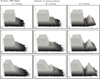 |
Fig. 7 Post-collapse morphology of a 30-m-high cliff made up of a high-friction 2:1 dust–ice mixture with a 3-m-thick sintered top layer for three different tilt angles of the overhang (columns) and of the crack (rows), respectively, (a) 10°, (b) 20°, (c) 30°. Steeper overhangs require a higher strength to be stable before triggering the collapse. Graphical representation as in Fig. 4. |
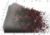 |
Fig. 8 Detailed view of the post-collapse morphology for the Aswan cliff collapse case. The pre-collapse cliff is made up of a 1:1 dust-ice mixture with a five-meter-thick sintered top layer. It is 130 m high and 80 m wide with an overhang of 20° and has a crack starting at half the cliff height with an opposite tilt angle of 10°. Only the debris pile is shown here. Graphical representation as in Fig. 4, but additionally with sinter bonds (thick red bars). The material is rendered partly transparent. |
 |
Fig. 9 Simulated tensile strength test. (a) A 10 cm-high and 5 cm-wide cylinder made up of a mixture of dust (gray spheres) and ice (blue spheres) particles is mounted in a clamp (a numerical wall with the shape of a truncated cone) with its flat top side, while a gradually increasing force is pulling on the cylinder’s flat bottom side until the cylinder breaks apart (shown here). (b) Time evolution of tensile stress for selected materials made up of particles with diameters of 1–2 mm. The horizontal dashed line pointing to the maximum of a curve is the stress at the breaking point, i.e., the material’s tensile strength σmax (values given in plot legend for each material). The oscillations in the early phase of the stress build-up result from longitudinal waves in the cylinder excited by the stepwise increase of the force pulling at the bottom. Their amplitudes decrease as the tension in the cylinder increases. Stresses measured during the preparation of the material samples are omitted for better representation. |
4.3 Tensile strength test
Proceeding as described in Sect. 3.3, we investigated the tensile strengths of materials with constituent size distributions and friction coefficients favored by the previous scenarios. We performed this test for all three dust-ice mixtures, with and without sintering of ice, for particles with diameters of 1–2 mm. As discussed in Sect. 4.1, the tensile strengths for the other particle sizes used in our simulations can be obtained by scaling with respect to the particle radius (∝ R−1). Figure 9 shows the recorded tensile stress diagrams, where the tensile strength is given by the maximum of the respective curve. Scaled with respect to our different used particle diameter ranges (from 10–20 mm to 0.2–0.4 mm), the resulting tensile strengths without sintering are in the range of 0.23–11 Pa (pure dust), 0.39–20 Pa (2:1 dust-ice volume ratio), and 0.47–23 Pa (1:1 dust-ice volume ratio), respectively, which shows the generally higher strength of the less porous, relatively ice-rich materials.
While we used “high friction” in these simulations, lower (higher) levels of friction can decrease (increase) the given numbers by several tens of percent. In contrast, in two additional simulations with a restitution coefficient of 0.1 and 0.8, respectively, instead of 0.3, the measured tensile strength differed by less than 1%, suggesting that the restitution coefficient has virtually no effect on tensile strength. This does not contradict the larger but still moderate influence of the restitution coefficient in the boulder drop tests, which are highly dynamic processes where energy dissipation plays a much more important role than in the quasi-static tensile strength test.
Additional tests with a timestep of 3% instead of 10% of the minimum of Rayleigh time and Hertz time resulted in less than 1% difference in the measured tensile strength of the material.
Sintering of ice has a comparatively small effect by increasing these values by less than 10%, which does not explain the partly surprisingly tough terrain observed for 67P’s consolidated areas (Spohn et al. 2015). We believe this is because of the porous and homogeneous structure of our materials, where the ice particles have only a few contacting neighbors (low coordination number) with less than half of them being other ice grains. For such a configuration, the formation of long sinter chains extending across many particles through large parts of the material is highly improbable. However, a still higher ice content and the associated stronger sintering effect can lead to much stronger materials. A series of numerical experiments for pure ice changing the sinter bond radius scaling factor  (0.01, 0.1, 0.5, 1.0) confirms that the macroscopic material’s tensile strength scales with
  as expected. However, in case of a low ice content, the lack of long sinter chains results only in a small dependence on
  . We note that our sintered low-ice-content boulders become rather more brittle than stable for increased
  , likely due to the reduced flexibility of the thicker sinter bonds while the overall dynamics is not yet governed by sinter bonds due to their relatively low number.
We also checked the applicability of the coarse-graining technique. The tensile strength of the cylinder was found to only weakly depend on the coarse-graining factor cg as long as the parcel number is generally not too small and not more than a few percent of the parcels are at the boundaries. Our results compare well with tensile strength estimates on the order of 10 Pa derived from Rosetta data (Groussin et al. 2015; Attree et al. 2018).
Parallel to the numerical simulations, tensile strength measurements have been performed in the laboratory (Haack et al. 2019, and in prep.). For this purpose, a different experimental setup in the form of the Brazilian disc test (Gundlach et al. 2018) was chosen, which is more suitable for handling weak and brittle materials under terrestrial conditions. Here, centimeter-sized disks of compacted test material are exposed to gradually increasing pressure against their curved side. The force at which a disk cracks can be used to calculate the material’s tensile strength. The utilized cometary analog materials were mixtures of polydisperse spherical silicate (fly ash) and water ice particles, with roughly power-law-distributed sizes but smaller power-law indexes of about ic = 1.5 and smaller mean diameters of about 4 μm than used in our numerical simulations. The experimental setup, including the material samples, was cooled with liquid nitrogen under terrestrial conditions to prevent sintering of the ice particles.
The tensile strength of pure water ice samples with a filling factor of ϕ = 0.74 was determined to 1800 Pa, which is compatible with similar experiments performed by Gundlach et al. (2018). Moreover, Haack et al. (2019, and in prep.) found a tensile strength of only 140 Pa for pure silicate samples at ϕ = 0.84. The strength of mixtures of both materials has proven to be close to the tensile strength of water ice and decreases tothe lower value of fly ash when the volume fraction of fly ash exceeds 75%. Scaling the tensile strengths of our model materials to the particle sizes used in the laboratory experiments gives values of ~400–1000 Pa. Although this neglects the influence of the different size distributions and filling factors, this is between the measured tensile strengths of pure fly ash and pure water ice, which demonstrates that our numerical results are compatible with laboratory measurements.
5 Conclusions and outlook
In this work, we applied the discrete element method (DEM) to perform numerical simulations of dynamical surface processes on comet 67P in order to investigate the mechanical properties of the surface material. We modeled our materials as different mixtures of polydisperse dust and water ice spheres and took into account the ambient surface acceleration, the Hertz contact model, translational and rolling friction, and cohesive forces from unsintered contacts, as well as sinter bonds between ice particles. To enable the modeling of large scenarios with realistically small constituent particles, we employed the coarse-graining technique, where an effective medium of computational parcels is considered, each parcel of radius cg R representing groups of several physical particles of radius R. Here, cg is referred to as the coarse-graining factor.
The presence of boulders on the surface of 67P requires the cometary bulk material to have a certain strength to sustain the ambient surface acceleration and survive drops from small heights, but also the possibility to break into fragments. In general, objects made of larger spherical particles are less stable, and increasing the friction between the particles leads to a less elastic, more brittle, but somewhat stronger material. From simulating the drop of two-meter-sized boulders from small heights, a reasonable behavior between total disintegration and no damage upon impact was observed for constituent particles with diameters on the order of 1 mm for a surface energy density of ω =0.028 J m−2. Changing the latter by a certain factor, the particle sizes have to be scaled by the same factor to approximately maintain the post-impact morphology. These observations can be carried over when heterogeneities are allowed by introducing locally more stable regions (e.g., smaller or less rough particles, higher coordination number). The breaking of boulders into large fragments and the formation of realistically rough debris fields required high levels of friction, which suggests that the constituents of the cometary bulk material are probably not all spherical but at least partly highly angular or very rough. This translates to weaker cohesive forces from unsintered contacts (asperity effect, Sect. 2.3), which has to be compensated by a correspondingly smaller particle size to again arrive at the same post-impact morphology.
We also investigated collapses of cliffs and overhangs of typical dimensions observed on 67P. For the DEM modeling, the cliff material was carried over from the boulder drop scenarios with the most realistic outcomes, such that the pre-collapse cliffs, which additionally exhibit a sintered top layer, are statically only just self-sustained. In the absence of material heterogeneities, we find that reasonable seismic activity generally does not suffice to trigger the collapses without resorting to a fine-tuning of parameters. In order to force a collapse, we introduced artificial cracks in the cliff material. Then, assuming otherwise homogeneous pre-collapse material, our numerical results suggest that most debris fields associated with collapses of cliffs on 67P probably originate from not overly strong and steep overhangs. However, the 67P observations are also compatible with heterogeneous pre-collapse materials or the occurrence of pre-collapse micro-cracks. In the case of a dedicated simulation of the Aswan cliff collapse, which was imaged on 67P before and after the event, we find the observed morphology to be compatible with our utilized material and mechanical parameters.
For our model materials, the influence of ice sintering on the material strength quadratically decreases with decreasing ice content. Sintering had a significant effect in the case of our ice-rich material (1:1 dust-to-ice-volume ratio) as it noticeably increased the overall strength and brittleness and led to a more distinct clustering of the post-impact and post-collapse debris. At very low dust-to-ice ratios, sintering can provide an explanation for the partly surprisingly tough terrain observed on 67P (Spohn et al. 2015). In contrast, other measurements (Fulle et al. 2017) suggest a global ice content that is lower than that of our ice-rich material and more similar to that of our ice-poor material (2:1 dust-to-ice-volume ratio), where sintering had a very small effect. However, the ice particles do not need to be distributed homogeneously across the comet, and in fact they are not (Oklay et al. 2017), such that it is still possible to have areas of weaker surface material mixed with areas of stronger surface material.
We also determined the tensile strengths of materials favored by the previous test scenarios. For this purpose, we pulled a cylinder made out of these materials to its breaking point. Not taking into account sintering, the calculated tensile strengths are in the range of 0.23–11 Pa (pure dust), 0.39–20 Pa (2:1 dust-ice volume ratio), and 0.47–23 Pa (1:1 dust-ice volume ratio), respectively, for our different particle diameter ranges (from 10–20 mm to 0.2–0.4 mm). A comparison of these measurements with the results from the boulder drops confirms a clear correlation between the tensile strength of the material and the stability of the boulders. In particular, we find that boulders made up of material with a tensile strength much larger than 10 Pa remain undamaged after impact, while boulders made up of material with a tensile strength much smaller than 1 Pa totally disintegrate. Sintering of ice increases these values by less than 10% for our considered dust–ice mixtures. Our results compare well with tensile strength estimates on the order of 10 Pa derived from Rosetta data (Groussin et al. 2015; Attree et al. 2018). They are also compatible with tensile strength measurements of cometary analogue materials Haack et al. (2019, and in prep.). This demonstrates that DEM modeling can be a powerful tool to investigate and constrain the macroscopic properties of cometary surface material. Once calibrated, numerical simulations can also be used to study problems that have been difficult to access experimentally such as the only partly explained mechanism of dust ejection from cometary surfaces (cometary activity paradox).
We find the coarse-graining technique to largely preserve the general trend in the tensile strength and the morphologic behavior. Here, the simulation outcomes have to be interpreted within tolerances given by slight changes in the geometric arrangement of the computational parcels at unchanged coarse-graining factor cg, which can by themselves, in a nonlinear way, lead to significant differences in the details of for example the fragmentation. Taking this into account, it proved to be successful to apply coarse-graining, as long as the parcel number is generally not too small and not more than a few percent of the parcels are at the boundaries. To improve the behavior in such cases, the simulation resolution has to be increased (i.e., cg decreased). Since the required computer memory scales with cg−3 and the computation time with cg−4, this approach has its limits. But it might be an option in future simulations to nonuniformly increase the resolution in the vicinity of existing boundaries and of expected new ones. Either way, we recommend to always, at least exemplarily, check the influence of coarse-graining on the simulation outcomes, in particular in cases where the fraction of parcels close to a boundary is not small.
In general, the details of the simulation outcomes (e.g., location and shape of cracks, exact number of fragments, trajectories of individual particles) can differ for slight changes in the numerical setup (e.g., initial microscopic geometrical arrangement of the particles, or order of summation given by choice of cutoff distance for the neighbor lists or by execution order when using parallel processing – the dependence on the summation order is a consequence of using finite precision floating point arithmetic which is not necessarily associative or distributive leading to noise in the numerical reproducibility). However, when again interpreted within tolerances as stated for the investigation of cg-changes, the boulder post-impact morphology was found to be only moderately sensitive when the coefficients of restitution of the parcels are changed from 0.3 to 0.1 or 0.8 or when increasing the Young’s modulus by a factor of ten. It was found to be weakly sensitive when the coefficient of restitution (Young’s modulus) of the bottom surface impacted by the boulder is changed from 0.3 to 0.1 (from 108 Pa to 107 Pa), when the impact angle of the boulder is changed from 30° to 0°, when moderately increasing the particle size range around a center particle radius, or when using a finer particle size binning. Weak sensitivity also resulted when setting the ratio of shear and tensile strength of bond cement to 0.3 instead of 1.0, when decreasing the time step from 10% of the minimum of Rayleigh and Hertz time to 3%, or when decreasing the neighbor list cutoff distances.
The morphologically most interesting boulder and cliff cases where the material broke into large (meter-sized) fragments with some debris occurred only for a comparatively small range of constituent sizes. One possible reason for this selective behavior could be the relatively narrow particle size distribution that we had to use because of the limited available computational resources (ratio of two between the largest and the smallest particle diameters) and our modeling assumption of a homogeneous material. This might have generated materials where the contact forces between the particles are still relatively uniform. As a result, the material totally disintegrates upon impact if the constituents are somewhat larger than a critical size or remains almost undamaged if the constituents are somewhat smaller than this size. Although the present situation is already improved compared to our earliest simulations with even narrower and more degenerate size distributions, this necessitated some fine-tuning to obtain a specific morphologic behavior. A possible solution for a more realistic simulation outcome where the level of fragmentation depends less critically on the constituent size could be to introduce local variations in the material properties.
A major source of uncertainty of our model is the assumed structure of the material, in particular the geometrical arrangement of the particles and their coordination number. We use a homogeneous mixture of two types of particles – dust and ice – that does not feature local variations in the arrangement of the particles or the material strength. Also, we do not consider the presence of small interstitial particles partially filling the voids between the larger particles and their potential cohesive effects. In reality, the cometary bulk material is most certainly not completely homogeneous and might have a structure that varies, possibly on different length scales. Since there is a high degeneracy between particle sizes, size distributions, and geometrical configuration as well as dust and ice abundance and mixing modalities, it is not possible at the present stage to draw definite conclusions on the dust-ice ratio on 67P from our DEM simulations alone. It always has to be kept in mind that the way dust and ice interact on 67P is much more complicated than we are able to model within the limits of our simulation setups.
An actual breaking (in contrast to a viscous deformation) of the bulk material forming our boulders needed high (rolling) friction between the particles. As mentioned above, since one of the main causes for rolling resistance are aspherical particle shapes, this suggests that the constituents of the cometary material are not all spherical, but include very rough, possibly even angular, interlocked particles. This is compatible with coma particles measured by the GIADA and MIDAS instruments aboard Rosetta partly showing highly complex aggregates (Fulle et al. 2015; Mannel et al. 2016) that probably originated from the nucleus surface. To better approximate such an almost fractal topology, we might need to introduce a further intermediate modeling level in addition to the basic coarse-graining technique employed inour simulations. Basic unsintered cohesive and frictional spherical particles on a micron scale would then be used to form complex agglomerates on a mesoscopic level, the mechanical properties of which (effective mesoscopic cohesion, friction, Young’s modulus, etc.) have to be explored by numerical experiments with several different realizations of such agglomerate blocks. These agglomerates are then treated as DEM building blocks in macroscopicscenarios, with properties as derived in the mesoscale experiments. This approach resembles the coarse-graining technique, but now with a refined focus on the details of the underlying microscopic material structure.
As the next step (Kappel et al. 2018a,b), we plan to study other surface processes on comet 67P that formed for example wind-tail-like structures and moats that have been observed around many exposed boulders (Mottola et al. 2015), and fracture polygons that have been observed in many places where consolidated material is exposed on the nucleus surface (Auger et al. 2018). We also intend to include Monte-Carlo-based modeling of sublimation and recondensation of volatiles and Knudsen gas flow through the surface layer, which will provide us with a tool to investigate more complex scenarios like triggers and early phases of cometary outbursts as well as other processes related to volatile compounds on comet 67P and other small Solar System bodies.
Acknowledgements
This work is part of the research project “The Physics of Volatile-Related Morphologies on Asteroids and Comets”. D.K., M.S., D.H., and K.O. would like to gratefully acknowledge the financial support and endorsement from the DLR Management Board Young Research Group Leader Program and the Executive Board Member for Space Research and Technology. We acknowledge the insightful comments and suggestions of an anonymous reviewer that greatly improved this work.
References
- Ai, J., Chen, J.-F., Rotter, J. M., & Ooi, J. Y. 2011, Powder Technol., 206, 269 [CrossRef] [Google Scholar]
- Attree, N., Groussin, O., Jorda, L., et al. 2018, A&A, 611, A33 [NASA ADS] [CrossRef] [EDP Sciences] [Google Scholar]
- Auger, A.-T., Groussin, O., Jorda, L., et al. 2018, Icarus, 301, 173 [NASA ADS] [CrossRef] [Google Scholar]
- Barthel, E. 2008, J. Phys. D: Appl. Phys., 41, 163001 [NASA ADS] [CrossRef] [Google Scholar]
- Basilevsky, A. T., Krasil’nikov, S. S., Shiryaev, A. A., et al. 2016, Sol. Syst. Res., 50, 225 [NASA ADS] [CrossRef] [Google Scholar]
- Bertini, I., Gutiérrez, P. J., Lara, L. M., et al. 2015, A&A, 583, A19 [NASA ADS] [CrossRef] [EDP Sciences] [Google Scholar]
- Bibring, J.-P., Langevin, Y., Carter, J., et al. 2015, Science, 349, aab0671 [CrossRef] [Google Scholar]
- Biele, J., Ulamec, S., Maibaum, M., et al. 2015, Science, 349, aaa9816 [NASA ADS] [CrossRef] [Google Scholar]
- Bierwisch, C., Kraft, T., Riedel, H., & Moseler, M. 2009, J. Mech. Phys. Solids, 57, 10 [NASA ADS] [CrossRef] [Google Scholar]
- Blackford, J. R. 2007, J. Phys. D Appl. Phys., 40, R355 [NASA ADS] [CrossRef] [Google Scholar]
- Blum, J., Gundlach, B., Krause, M., et al. 2017, MNRAS, 469, S755 [CrossRef] [Google Scholar]
- Brilliantov, N. V., Spahn, F., Hertzsch, J.-M., & Pöschel, T. 1996, Phys. Rev. E, 53, 5382 [Google Scholar]
- Brownlee, D. E., Horz, F., Newburn, R. L., et al. 2004, Science, 304, 1764 [NASA ADS] [CrossRef] [PubMed] [Google Scholar]
- Capaccioni, F., Coradini, A., Filacchione, G., et al. 2015, Science, 347, aaa0628 [Google Scholar]
- Castellanos, A. 2005, Adv. Phys., 54, 263 [Google Scholar]
- Cheng, B., Yu, Y., & Baoyin, H. 2017, Sci. Rep., 7, 10004 [NASA ADS] [CrossRef] [Google Scholar]
- Cheng, B., Yu, Y., & Baoyin, H. 2019, MNRAS, 485, 3088 [NASA ADS] [CrossRef] [Google Scholar]
- Colwell, J. E. 1993, Lunar Planet. Sci. Conf., 24, 325 [Google Scholar]
- Cundall, P. A., & Strack, O. D. L. 1979, Géotechnique, 29, 47 [CrossRef] [Google Scholar]
- DCS Computing GmbH 2016, LIGGGHTS User Manual [Google Scholar]
- Di Renzo, A., & Di Maio, F. P. 2004, Chem. Eng. Sci., 59, 525 [CrossRef] [Google Scholar]
- Di Renzo, A., & Di Maio, F. P. 2005, Chem. Eng. Sci., 60, 1303 [CrossRef] [Google Scholar]
- El-Maarry, M. R., Thomas, N., Giacomini, L., et al. 2015, A&A, 583, A26 [NASA ADS] [CrossRef] [EDP Sciences] [Google Scholar]
- El-Maarry, M. R., Thomas, N., Gracia-Berná, A., et al. 2016, A&A, 593, A110 [NASA ADS] [CrossRef] [EDP Sciences] [Google Scholar]
- El-Maarry, M. R., Thomas, N., Gracia-Berná, A., et al. 2017, A&A, 598, C2 [NASA ADS] [CrossRef] [EDP Sciences] [Google Scholar]
- El-Maarry, M. R., Groussin, O., Keller, H. U., et al. 2019, Space Sci. Rev., 215, 36 [CrossRef] [Google Scholar]
- Fornasier, S., Hasselmann, P. H., Barucci, M. A., et al. 2015, A&A, 583, A30 [NASA ADS] [CrossRef] [EDP Sciences] [Google Scholar]
- Fuller, K. N. G., & Tabor, D. 1975, Proc. R. Soc. London Ser. A, 345, 327 [NASA ADS] [CrossRef] [Google Scholar]
- Fulle, M., Corte, V. D., Rotundi, A., et al. 2015, ApJ, 802, L12 [NASA ADS] [CrossRef] [Google Scholar]
- Fulle, M., Della Corte, V., Rotundi, A., et al. 2016, MNRAS, 462, S132 [CrossRef] [Google Scholar]
- Fulle, M., Della Corte, V., Rotundi, A., et al. 2017, MNRAS, 469, S45 [Google Scholar]
- Gold, L. W. 1958, Can. J. Phys., 36, 1265 [NASA ADS] [CrossRef] [Google Scholar]
- Groussin, O., Jorda, L., Auger, A. T., et al. 2015, A&A, 583, A32 [NASA ADS] [CrossRef] [EDP Sciences] [Google Scholar]
- Gulkis, S., Allen, M., Allmen, P. v., et al. 2015, Science, 347, aaa0709 [Google Scholar]
- Gundlach, B., Schmidt, K. P., Kreuzig, C., et al. 2018, MNRAS, 479, 1273 [NASA ADS] [CrossRef] [Google Scholar]
- Haack, D., Otto, K., Kührt, E., et al. 2019, EPSC-DPS Joint Meeting, 13, EPSC [Google Scholar]
- Haas, C. J. 1989, Static Stress-strain Relationships, ed. C. Ho5210 (New York: Hemisphere Publishing), 123 [Google Scholar]
- Heim, L.-O., Blum, J., Preuss, M., & Butt, H.-J. 1999, Phys. Rev. Lett., 83, 3328 [NASA ADS] [CrossRef] [Google Scholar]
- Hertz, H. 1882, Journal für die reine und angewandte Mathematik, 92, 156 [Google Scholar]
- Hirabayashi, M., Sánchez, D. P., & Scheeres, D. J. 2015, ApJ, 808, 63 [NASA ADS] [CrossRef] [Google Scholar]
- Hobbs, P. 1974, Ice Physics (Oxford: Clarendon Press) [Google Scholar]
- Holsapple, K. A., & Housen, K. R. 2007, Icarus, 191, 586 [CrossRef] [Google Scholar]
- Hviid, S. F., Hüttig, C., Groussin, O., et al. 2016, AAS/Div. Planet. Sci.Meeting Abs., 48, 211.05 [Google Scholar]
- Johnson, K. L., Kendall, K., & Roberts, A. D. 1971, Proc. Roy. Soc. London Ser. A, 324, 301 [NASA ADS] [Google Scholar]
- Jorda, L., Gaskell, R., Capanna, C., et al. 2016, Icarus, 277, 257 [NASA ADS] [CrossRef] [Google Scholar]
- Kappel, D., Otto, K., Oklay-Vincent, N., et al. 2018a, Lunar Planet. Sci. Conf., 49, 2696 [Google Scholar]
- Kappel, D., Otto, K., Oklay, N., et al. 2018b, Euro. Planet. Sci. Cong., 12, EPSC2018 [Google Scholar]
- Keller, H. U., Barbieri, C., Lamy, P., et al. 2007, Space Sci. Rev., 128, 433 [NASA ADS] [CrossRef] [Google Scholar]
- Keller, H. U., Mottola, S., Davidsson, B., et al. 2015, A&A, 583, A34 [NASA ADS] [CrossRef] [EDP Sciences] [Google Scholar]
- Keller, H. U., Mottola, S., Hviid, S. F., et al. 2017, MNRAS, 469, S357 [CrossRef] [Google Scholar]
- Kimura, H., Wada, K., Senshu, H., & Kobayashi, H. 2015, ApJ, 812, 67 [NASA ADS] [CrossRef] [Google Scholar]
- Kleinhans, M. G., Markies, H., de Vet, S. J., in’t Veld, A. C., & Postema, F. N. 2011, J. Geophys. Res. Planets, 116, E11004 [CrossRef] [Google Scholar]
- Kloss, C., Goniva, C., Hager, A., Amberger, S., & Pirker, S. 2012, Prog. Comput. Fluid Dyn., 12, 140 [Google Scholar]
- Knapmeyer, M., Fischer, H. H., Knollenberg, J., et al. 2018, Icarus, 310, 165 [NASA ADS] [CrossRef] [Google Scholar]
- Kofman, W., Herique, A., Barbin, Y., et al. 2015, Science, 349, 2.639 [NASA ADS] [CrossRef] [Google Scholar]
- Kokelaar, B. P., Bahia, R. S., Joy, K. H., Viroulet, S., & Gray, J. M. N. T. 2017, J. Geophys. Res. Planets, 122, 1893 [NASA ADS] [CrossRef] [Google Scholar]
- Küppers, M., Keller, H. U., Kührt, E., et al. 2009, Exp. Astron., 23, 809 [CrossRef] [Google Scholar]
- Leite, F. L., Bueno, C. C., Da Róz, A. L., Ziemath, E. C., & Oliveira, O. N. 2012, Int. J. Mol. Sci., 13, 12773 [CrossRef] [Google Scholar]
- Maeno, N., & Ebinuma, T. 1983, J. Phys. Chem., 87, 4103 [CrossRef] [Google Scholar]
- Mannel, T., Bentley, M. S., Schmied, R., et al. 2016, MNRAS, 462, S304 [NASA ADS] [CrossRef] [Google Scholar]
- Martin, C. L., & Bordia, R. K. 2008, Phys. Rev. E, 77, 031307 [NASA ADS] [CrossRef] [Google Scholar]
- Matonti, C., Attree, N., Groussin, O., et al. 2019, Nat. Geosci., 12, 157 [NASA ADS] [CrossRef] [Google Scholar]
- Mellon, M. T. 1997, J. Geophys. Res., 102, 25617 [NASA ADS] [CrossRef] [Google Scholar]
- Molaro, J. L., Choukroun, M., Phillips, C. B., et al. 2019, J. Geophys. Res. Planets, 124, 243 [NASA ADS] [CrossRef] [Google Scholar]
- Mottola, S., Arnold, G., Grothues, H.-G., et al. 2015, Science, 349, aab0232 [CrossRef] [Google Scholar]
- Muller, V., Derjaguin, B., & Toporov, Y. 1983, Colloids Surf., 7, 251 [CrossRef] [Google Scholar]
- Oklay, N., Mottola, S., Vincent, J.-B., et al. 2017, MNRAS, 469, S582 [CrossRef] [Google Scholar]
- Pajola, M., Vincent, J.-B., Güttler, C., et al. 2015, A&A, 583, A37 [NASA ADS] [CrossRef] [EDP Sciences] [Google Scholar]
- Pajola, M., Oklay, N., Forgia, F. L., et al. 2016, A&A, 592, A69 [NASA ADS] [CrossRef] [EDP Sciences] [Google Scholar]
- Pajola, M., Höfner, S., Vincent, J. B., et al. 2017, Nat. Astron., 1, 0092 [CrossRef] [Google Scholar]
- Potyondy, D., & Cundall, P. 2004, Int. J. Rock Mech. Mining Sci., 41, 1329 [Google Scholar]
- Preusker, F., Scholten, F., Matz, K. D., et al. 2017, A&A, 607, L1 [NASA ADS] [CrossRef] [EDP Sciences] [Google Scholar]
- Radl, S., Radeke, C., Khinast, J., & Sundaresan, S. 2011, in 8th International Conference on CFD in Oil & Gas, Metallurgical and Process Industries [Google Scholar]
- Richardson, J. E., Melosh, H. J., Greenberg, R. J., & O’Brien, D. P. 2005, Icarus, 179, 325 [NASA ADS] [CrossRef] [Google Scholar]
- Richter, C. 2015, LIGGGHTS-WITH-BONDS, https://github.com/richti83/LIGGGHTS-WITH-BONDS [Google Scholar]
- Rotundi, A., Sierks, H., Corte, V. D., et al. 2015, Science, 347, aaa3905 [NASA ADS] [CrossRef] [Google Scholar]
- Scheeres, D. J., Hartzell, C. M., Sánchez, P., & Swift, M. 2010, Icarus, 210, 968 [NASA ADS] [CrossRef] [Google Scholar]
- Schultz, R. A. 1995, Rock Mech. Rock Eng., 28, 1 [Google Scholar]
- Schwartz, S. R., Michel, P., Jutzi, M., et al. 2018, Nat. Astron., 2, 379 [NASA ADS] [CrossRef] [Google Scholar]
- Sierks, H., Barbieri, C., Lamy, P. L., et al. 2015, Science, 347, aaa1044 [Google Scholar]
- Silbert, L. E., Ertas, D., Grest, G. S., et al. 2001, Phys. Rev. E, 64, 051302 [Google Scholar]
- Spohn, T., Knollenberg, J., Ball, A. J., et al. 2015, Science, 349, aab0464 [NASA ADS] [CrossRef] [Google Scholar]
- Squyres, S. W., Nakamura-Messenger, K., Mitchell, D. F., et al. 2018, Lunar Planet. Sci. Conf., 49, 1332 [Google Scholar]
- Sunshine, J. M., Thomas, N., El-Maarry, M. R., & Farnham, T. L. 2016, J. Geophys. Res. Planets, 121, 2194 [NASA ADS] [CrossRef] [Google Scholar]
- Swope, W. C., Andersen, H. C., Berens, P. H., & Wilson, K. R. 1982, J. Chem. Phys., 76, 637 [NASA ADS] [CrossRef] [Google Scholar]
- Tancredi, G., Maciel, A., Heredia, L., Richeri, P., & Nesmachnow, S. 2012, MNRAS, 420, 3368 [NASA ADS] [CrossRef] [Google Scholar]
- Teanby, N. A., & Wookey, J. 2011, Phys. Earth Planet. Interiors, 186, 70 [CrossRef] [Google Scholar]
- Thomas, N., Sierks, H., Barbieri, C., et al. 2015a, Science, 347, aaa0440 [CrossRef] [Google Scholar]
- Thomas, N., Davidsson, B., El-Maarry, M. R., et al. 2015b, A&A, 583, A17 [NASA ADS] [CrossRef] [EDP Sciences] [Google Scholar]
- Vincent, J.-B., Bodewits, D., Besse, S., et al. 2015, Nature, 523, 63 [NASA ADS] [CrossRef] [Google Scholar]
- Vincent, J.-B., Oklay, N., Pajola, M., et al. 2016, A&A, 587, A14 [NASA ADS] [CrossRef] [EDP Sciences] [Google Scholar]
- Vincent, J.-B., Birch, S., Hayes, A., et al. 2019, EPSC-DPS Joint Meeting, 13, EPSC [Google Scholar]
All Tables
All Figures
|
Fig. 1 Examples of morphologic features on comet 67P as imaged by the OSIRIS narrow-angle camera (Keller et al. 2007). (a) Hathor cliff with boulders accumulating at the airfall-covered foot of the cliff. The consolidated tough material of the cliff supports an escarpment height of about 900 m. The largest boulders are approximately 50 m across. (b) Pre-collapse Aswan plateau and cliff site with smooth airfall deposits, consolidated wall material, and debris with boulders at the cliff foot (center left). The shadowed pit in the top left of the image is approximately 200 m across. (c) Foot of a collapsed debris field populated with boulders up to 10–15 m across. (d) Debris deposits superimposing an apparently smooth region of small airfall particles. Bare consolidated and airfall-covered terrains alternate spatially. The boulder deposit in the upper left and the airfall-covered plateau in the center of the image are each approximately 500 m wide. Figure tags: (a) NAC_ 2014-09-29T08.52.08.332Z_ID30_1397549001_F41, (b) NAC_2014-09-29T16.10.04.817Z_ID30_1397549000_F16, (c) NAC_2016-08-03T07.28.34.758Z_ID30_1397549000_F22, (d) NAC_2014-09-13T23.29.22.367Z_ID30_1397549001_F41. Credits: ESA/Rosetta/MPS for OSIRIS Team MPS/UPD/LAM/IAA/SSO/INTA/UPM/DASP/IDA. |
| In the text | |
|
Fig. 2 Construction and simulated drop of a sintered two-meter-sized boulder made up of a 2:1 dust–ice mixture (34 000 computational parcels) from 30 m above the surface (beige-colored plane) of comet 67P. Oblique impact with impact speed of 0.1 m s−1 and impact angle of 30° measured from the normal to the surface. Top row: construction of the boulder. (a) Loose filling of a large sphere with noncontacting randomly sized and positioned dust (gray spheres) and ice (blue spheres) particles. (b) Compaction of the boulder to the bulk mass density and porosity of comet 67P. (c) Removal of particles outside the intended boulder diameter and formation of sinter bonds (thick red bars) between ice particles. Bottom row: (d–f) Several stages after impacting the surface of 67P; sinter bond representation is omitted for clarity. Lighter shades of gray or blue visualize a higher topography. In case (c), the material is visualized partly transparent. |
| In the text | |
|
Fig. 3 Construction and simulated collapse of a 30-m-high cliff made up of a 2:1 dust–ice mixture (65 000 computational parcels) with a sintered top layer of 3 m thickness. Top row: construction of the cliff. (a) Loose filling of a region confined by walls with noncontacting randomly sized and positioned dust (gray spheres) and ice (blue spheres) particles. (b) Compactionof the cliff to the bulk mass density and porosity of comet 67P. (c) Removal of particles beyond the given cliff height, formation of sinter bonds (thick red bars) between ice particles in the top layer of the cliff, and removal of the wall supporting the overhang. Bottom row: (d–f) Several stages after triggering the collapse. Representation as in Fig. 2. Particles in white are from the initial crack region. |
| In the text | |
|
Fig. 4 Post-impact morphology of dropped two-meter-sized boulders made up of dust particles from different size ranges (rows). Impact conditions and graphical representation as in Fig. 2, but the indication of the particle type (water ice vs. dust) by colors is omitted for clarity here and in the following. Left column: low friction. Mid column: high friction. Right column: very high friction. |
| In the text | |
|
Fig. 5 Post-impact morphology of dropped two-meter-sized boulders made up of a 2:1 dust–ice mixture of particles from different size ranges (rows) and under different friction and sintering conditions (columns). Impact conditions and graphical representation as in Fig. 4. |
| In the text | |
|
Fig. 6 Post-impact morphology of dropped two-meter-sized boulders made up of a 1:1 dust–ice mixture of particles from different size ranges (rows) and under different friction and sintering conditions (columns). Impact conditions and graphical representation as in Fig. 4. |
| In the text | |
|
Fig. 7 Post-collapse morphology of a 30-m-high cliff made up of a high-friction 2:1 dust–ice mixture with a 3-m-thick sintered top layer for three different tilt angles of the overhang (columns) and of the crack (rows), respectively, (a) 10°, (b) 20°, (c) 30°. Steeper overhangs require a higher strength to be stable before triggering the collapse. Graphical representation as in Fig. 4. |
| In the text | |
|
Fig. 8 Detailed view of the post-collapse morphology for the Aswan cliff collapse case. The pre-collapse cliff is made up of a 1:1 dust-ice mixture with a five-meter-thick sintered top layer. It is 130 m high and 80 m wide with an overhang of 20° and has a crack starting at half the cliff height with an opposite tilt angle of 10°. Only the debris pile is shown here. Graphical representation as in Fig. 4, but additionally with sinter bonds (thick red bars). The material is rendered partly transparent. |
| In the text | |
|
Fig. 9 Simulated tensile strength test. (a) A 10 cm-high and 5 cm-wide cylinder made up of a mixture of dust (gray spheres) and ice (blue spheres) particles is mounted in a clamp (a numerical wall with the shape of a truncated cone) with its flat top side, while a gradually increasing force is pulling on the cylinder’s flat bottom side until the cylinder breaks apart (shown here). (b) Time evolution of tensile stress for selected materials made up of particles with diameters of 1–2 mm. The horizontal dashed line pointing to the maximum of a curve is the stress at the breaking point, i.e., the material’s tensile strength σmax (values given in plot legend for each material). The oscillations in the early phase of the stress build-up result from longitudinal waves in the cylinder excited by the stepwise increase of the force pulling at the bottom. Their amplitudes decrease as the tension in the cylinder increases. Stresses measured during the preparation of the material samples are omitted for better representation. |
| In the text | |
Current usage metrics show cumulative count of Article Views (full-text article views including HTML views, PDF and ePub downloads, according to the available data) and Abstracts Views on Vision4Press platform.
Data correspond to usage on the plateform after 2015. The current usage metrics is available 48-96 hours after online publication and is updated daily on week days.
Initial download of the metrics may take a while.