| Issue |
A&A
Volume 640, August 2020
|
|
|---|---|---|
| Article Number | L21 | |
| Number of page(s) | 7 | |
| Section | Letters to the Editor | |
| DOI | https://doi.org/10.1051/0004-6361/202038785 | |
| Published online | 28 August 2020 | |
Letter to the Editor
Early warning signals indicate a critical transition in Betelgeuse
1
University of Groningen, University Medical Center Groningen (UMCG), Groningen, Department of Psychiatry, Interdisciplinary Center Psychopathology and Emotion regulation (ICPE), Groningen, The Netherlands
e-mail: This email address is being protected from spambots. You need JavaScript enabled to view it.
2
Indian Institute of Science Education and Research (IISER) Tirupati, Tirupati 517507, India
3
Inter University Centre for Astronomy and Astrophysics (IUCAA), Pune 411007, India
Received:
29
June
2020
Accepted:
3
August
2020
Abstract
Context. Critical transitions occur in complex dynamical systems when the system dynamics undergoes a regime shift. These can often occur with little change in the mean amplitude of the system response prior to the actual time of transition. The recent dimming and brightening event in Betelgeuse occurred as a sudden shift in the brightness and has been the subject of much debate. Internal changes or an external dust cloud have been suggested as reasons for this change in variability.
Aims. We examine whether the dimming and brightening event of 2019–20 could be due to a critical transition in the pulsation dynamics of Betelgeuse by studying the characteristics of the light curve prior to transition.
Methods. We calculated the quantifiers hypothesized to rise prior to a critical transition for the light curve of Betelgeuse up to the dimming event of 2019–20. These included the autocorrelation at lag-1, variance, and the spectral coefficient calculated from detrended fluctuation analysis, in addition to two measures that quantify the recurrence properties of the light curve. Significant rises are confirmed using the Mann-Kendall trend test.
Results. We see a significant increase in all quantifiers (p < 0.05) prior to the dimming event of 2019–20. This suggests that the event was a critical transition related to the underlying nonlinear dynamics of the star.
Conclusions. Together with results that suggest a minimal change in Teff and IR flux, a critical transition in the pulsation dynamics might be a reason for the unprecedented dimming of Betelgeuse. The rise in the quantifiers we studied prior to the dimming event supports this possibility.
Key words: stars: individual: α Orionis / methods: data analysis / stars: variables: general
© ESO 2020
1. Introduction
Betelgeuse, or α Orionis, is a fascinating supergiant whose variability has been of particular interest to astronomers. As a semiregular variable star, Betelgeuse usually varies in visual magnitude from 0.6 to 1.1 approximately every 425 days, with some evidence of a longer 5.9-year period (Goldberg 1984; Samus et al. 2017; Dupree et al. 1987; Stothers & Leung 1971). This rapidly evolving supergiant that is well off the main sequence is particularly exciting to study, since quasi-hydrostatic evolutionary models predict that it will undergo a supernova explosion sometime in the next 100 000 years (Dolan et al. 2016).
The interest in this star suddenly increased at the end of 2019 because a strong dimming and subsequent rapid brightening event took place (Guinan & Wasatonic 2020; Sigismondi 2020a). The dimming reported by Guinan et al. (2019) reignited the questions related to the internal dynamics of this red supergiant (RSG) and led to speculations regarding an impending supernova explosion. Multiple hypotheses have been suggested in order to explain this dimming, which was recorded as the dimmest that the star has been in its observational history. Proposed explanations for the dimming phenomenon include an increase in the circumstellar dust or cooling in convective cells (Levesque & Massey 2020). Some authors have also noted that the dimming coincides with the minimum in the 2300-day and 400-day periodicities of the star (Sigismondi 2020b; Percy 2020). The hypothesis that the dimming is due to variation in the convective cells has been refuted by a measurement of the surface temperature of the star, which showed no significant difference between the Teff measured in 2004 and near the minimum in 2020 (Levesque & Massey 2020). This suggested that a dust cloud must be responsible for the rapid dimming of the star. The circumstellar envelope around Betelgeuse was previously observed and characterized by Haubois et al. (2019). Gupta & Sahijpal (2020) further characterized the nature of the dust grains that can condense in this circumstellar envelope. While initial measurements by Cotton et al. (2020) during the dimming phase indicated a reduction in polarization, detailed analysis suggested that the polarized flux from the envelope remained constant during the dimming, and subsequently increased during the brightening (Safonov et al. 2020). Safonov et al. (2020) suggested that a dust cloud would result in an IR excess close to the dimming. However, measurements by Gehrz et al. (2020) during the dimming episode in the IR region inferred that no significant change in flux was observed. This was further supported by observations in the submillimeter wavelength by Dharmawardena et al. (2020).
A critical transition occurs in a nonlinear dynamical system when the nature of the system dynamics undergoes a drastic change. In dynamical systems theory, the point where this transition occurs is called a bifurcation point (Hilborn 2000). Very often, these critical transitions can take place with no visible variation in the mean amplitude in the system dynamics prior to the point of actual transition. This makes these changes difficult to predict.
One of the possibilities for the sudden dimming of Betelgeuse could be a critical transition in the pulsation dynamics of the star. Pulsation has long been understood as a cause of variability in Betelgeuse (Dupree et al. 1987). Variability due to stellar pulsations in many stars has been modeled using nonlinear dynamical models (Baker & Gough 1979; Kolláth et al. 2002). A transition in the pulsation dynamics of Betelgeuse can be captured using nonlinear time-series analysis techniques on the light curve of the star. Nonlinear time-series analysis has been used in multiple fields of astronomy, and for stellar variability in particular (Lindner et al. 2015; George et al. 2015; Plachy et al. 2018). An important application of nonlinear time-series analysis has been made in the prediction of critical transitions in real-world systems.
A dynamical system can exist in one of its many possible states, each of which may have a distinct pattern of evolution and occurs for a particular range of system parameters. When the parameters change beyond this range, the dynamical state of the system changes to another state. This phenomenon, called a dynamical transition, results in a qualitative change in the dynamical behavior of the system. Critical transitions in dynamical systems can take place even with minor changes in these parameter values. Such critical transitions would lead to major changes in the dynamical behavior of the system (Hilborn 2000). For instance, a Hopf bifurcation would lead to the birth of sudden periodic behavior. Seminal work by Scheffer et al. (2009) suggested that prior to a critical transition in a dynamical system, multiple time-series quantifiers increase (Scheffer et al. 2009, 2012). In particular the autocorrelation at lag-1, the variance, and the spectral exponent have been shown to increase prior to a transition. This has been used to predict dynamical transitions in many fields, including ecology, engineering, and psychiatry (Dakos et al. 2012; Lenton et al. 2012; Trefois et al. 2015; Ghanavati et al. 2014; Wichers & Groot 2016; Shalalfeh et al. 2016).
Another way to detect a change in the dynamics of a system is to examine the associated phase space. Structures in phase space trace the evolution of the system in a way that can be quantified in terms of density and recurrence of points in time. The pattern of return or recurrences can be analyzed using what is known as recurrence quantification analysis (RQA; Marwan et al. 2007). This pattern of return times is known to change near critical transitions (Wissel 1984), which reflects as changes in RQA measures. RQA measures have been used for the characterization of system dynamics in different domains such as climate studies (Zhao et al. 2011), physiological data analysis (Acharya et al. 2011; Marwan et al. 2002), stock markets (Bastos & Caiado 2011), and engineering (Godavarthi et al. 2017). They have been particularly useful for the identification of dynamical transitions, including periodic-chaos and chaos-chaos transitions, as well as intermittent states (Marwan et al. 2013; Godavarthi et al. 2017).
In stellar variability, critical transitions often take place at timescales that are much longer than the period of observation. The event of 2019–20 in Betelgeuse is a welcome exception. We examine the variation of these quantifiers in the light curve of Betelgeuse from 1990–2019 up to the transition. We then search for significant variations in these quantifiers over time. If the dimming and subsequent brightening event of 2019–20 was due to internal factors leading to a critical transition in the pulsation dynamics of the star, we expect a detectable increase in these quantifiers.
2. Early warning signals in Betelgeuse
Transitions in dynamics are characteristic of complex nonlinear dynamical systems, whereby the dynamics of the system undergoes a regime shift. Many of these sharp transitions are preceded by early warning signals in the system response. A positive feedback loop drives the system forward to a bifurcation point after a critical threshold is achieved (Scheffer et al. 2009). Two quantifiers that are hypothesized to rise in this scenario are the variance and the autocorrelation at lag-1 (ACF(1)). A closely related quantifier is the detrended fluctuation analysis (DFA) exponent α, which measures long-term memory in the time series (Peng et al. 1994). Briefly, the detrended fluctuation analysis initially transforms the data into a time series of the cumulative amplitude distribution. The fluctuation (determined as the root mean squared deviation) of this cumulative time series from the linear trend is calculated at different timescales. This fluctuation is expected to rise as a power law with respect to the timescale considered, the exponent of which is the Hurst exponent, α (Peng et al. 1994; Livina & Lenton 2007; Shalalfeh et al. 2016). A sudden shift in the observed response of a system need not necessarily be preceded by an early warning signal. For instance, a sudden change in the observational data, caused by some external influences, may not show any warning signals. Even for sudden observational shifts caused by dynamical transitions, only some are clearly preceded by early warning signals. However, early warning signals, if detected in a system, can be taken as a good indication of a possible approaching transition (Scheffer et al. 2012).
For our analysis we used light-curve data from the American Association of Variable Star Observers (AAVSO; Kafka 2020). The light curve of Betelgeuse was binned into ten-day bins to examine the long trends in the data. As mentioned earlier, we quantified the lag-1 autocorrelation, the variance, and the Hurst exponent α (Scheffer et al. 2009; Livina & Lenton 2007).
The quantifiers were calculated over moving windows with a size of 300 points. The window was moved forward by one data point, regardless of gaps. A study across different window sizes was conducted, and the results are shown in Appendix C. While the effect sizes decreased for individual quantifiers, especially at small window sizes, the broad conclusions remain unchanged. All calculations were conducted in python 3.5.2 using the numpy, scipy, and entropy packages (Oliphant 2006; Virtanen et al. 2020; Vallat 2020).
Missing data are a cause for concern in this dataset, as Betelgeuse is not observable for a long period between May and July. However, if stationarity is assumed at the timescales of the size of the gaps, calculations of the variance and ACF(1) should not be affected much by missing data. Furthermore, the Hurst exponent α has been shown to be very robust to missing data in positively correlated data (Ma et al. 2010). The profile of gaps in the AAVSO dataset and its variation with time is considered in Appendix A. Because of the many gaps in the period from 1980–1990, trends were analyzed for the period starting from 1990 onward.
To determine trends in the quantifiers, we examined the Kendall correlation coefficient (τK) up to the transition point. To correct for correlation due to the moving-window approach, we used the Hamed-Rao correction (Hamed & Rao 1998). Calculations were conducted using the pymannkendall package in python (Hussain & Mahmud 2019). Increasing trends are seen for all three quantifiers with time prior to the transition in brightness, indicating that a dynamical transition in Betelgeuse led to the 2019–20 dimming and brightening event. The trends, values of τK, and p-values are listed in Table 1. The change in the early warning signals with time are shown in Fig. 1. The gray region (1980–90 data) in Fig. 1 shows an increased variance and α prior to the period considered. Joyce et al. (2020) pointed out a major dimming event in the mid to late 1980s, which may be a possible explanation for the change in these quantifiers around that period. In the next section, we supplement the warning signals we detected in this section with quantifiers derived using recurrence quantification analysis.
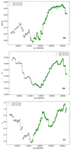 |
Fig. 1. Variation in (panel a) autocorrelation at lag-1, (panel b) variance, and (panel c) spectral coefficient, α, calculated from detrended fluctuation analysis prior to the dimming event. The period from 1980–1990 is shown in gray, and the period from 1990 onward is shown in green. A visible rise can be seen leading towards the event. The calculated quantifier is plotted at the end time of the moving window. |
Significant increases in early warning signals prior to the dimming event in Betelgeuse data.
3. Recurrence-based analysis
Recurrence-based measures have been applied for the study of black holes (Jacob et al. 2018), variable stars (George et al. 2019), solar radiation (Ogunjo et al. 2017), and exoplanetary systems (Kovács 2019). A rather remarkable advantage of RQA measures is their ability to detect dynamical transitions from a time series even when the details of the underlying dynamics are elusive (Marwan et al. 2013; Thiel et al. 2004). Recurrence-based measures are successful even with nonstationary and short datasets (Marwan et al. 2007).
The time series was first transformed into an attractor in phase space by what is known as delay embedding (Kantz & Schreiber 2004; Takens 1981). The process generates an attractor in phase space that is topologically equivalent to the original attractor and captures evolution of the system for the duration of a given time series. Every point on the attractor is considered a vector, and a distance matrix is constructed that encapsulates recurrences in the system in terms of distances between the vectors. When we apply a threshold to the distance metric such that the points within the threshold are considered close, then we obtain the recurrence matrix, R. Each element of R corresponds to a unique pair of points in the phase space, and the value of 1 indicates their proximity (0 otherwise). The visual representation of R, with zeros as white dots and ones as black dots is a recurrence plot (RP).
The RP for the entire time series of Betelgeuse for the duration 1980 up to just before the dimming event in 2019 is shown in Fig. 2 for illustration. The moving-window approach considers segments of the time series, however, and the corresponding RPs are constructed for each window. We fixed the recurrence threshold such that the recurrence rate remained at 0.1 and calculated other quantifiers. The exact definitions along with the parameters we used for the construction of the RP are given in Appendix B.
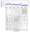 |
Fig. 2. Recurrence plot of the time series of Betelgeuse. Upper panel: corresponding time series (in blue). The red part (dimming) was not included in the analysis. The parameters used are m = 1, τ = 1, and fixed RR = 0.1. |
The RQA measures assess the patterns formed by points, diagonal lines, vertical lines, and other structures in the RP. RQA measures such as the recurrence rate (RR), determinism (DET), and laminarity (LAM) are intimately related to the underlying dynamics: RR computes the number of recurred states (based on the number of recurrence points), DET estimates how deterministic the dynamics appears to be (based on the distribution of diagonal lines in the RP), and LAM reflects the extent of laminar phases in the system (based on the distribution of white vertical lines), or intermittency. In the case of a dynamical transition, the values should deviate significantly from an overall average calculated with the assumption of no transition (Marwan et al. 2013; Schinkel et al. 2009).
The behavior of these measures is shown in Fig. 3. Laminarity and DET both increase systematically as the dimming episode approaches and appear to follow a similar trend overall. The results quantifying the change in the DET and LAM measures with time using the modified Mann-Kendall test is shown in Table 2 (Hamed & Rao 1998). The test confirms a significant gradual increase in the measures. We observe that the measures of DET and LAM exceed the 95% confidence level (obtained from 1000 bootstrappings, as suggested by Schinkel et al. 2009) before the dimming with LAM slightly rises before DET. This behavior can be expected from intermittency (reflected in the high value of the LAM) associated with the phenomenon of critical slowing down that leads to a dynamical shift (significant change in DET).
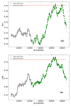 |
Fig. 3. Variation in RQA measures (panel a) DET and (panel b) LAM prior to the dimming event for fixed RR = 0.1. The red line indicates the 95% confidence level. The color code is similar to that in Fig. 1. The gray region refers to 1980–1990. |
Significant increases in RQA measures prior to the dimming event in Betelgeuse data.
4. Results and discussion
We analyzed the light curve of Betelgeuse from 1990 until the dimming event. Our analysis suggests that signatures of an impending change in the nonlinear dynamics can be observed from the properties of the light curve preceding the dimming episode. The quantifiers we used, which are employed in the literature on early warning signals and recurrence-based analysis, showed conclusively that certain properties of the light curve changed significantly prior to the dimming event in 2019. The rise in early warning signals prior to the dimming episode in late 2019 was quantified using the Mann-Kendall test, which checks the correlation of the quantifiers with time. Along with classically used early warning quantifiers, we also studied the variation in the recurrence-based quantifiers. These independently show a change prior to the dimming event. A comparison between the two suggests that the change in quantifiers started at about the same time.
This result has a significant effect on our understanding of the 2019 dimming event. The observations in the submillimeter wavelengths reported by Dharmawardena et al. (2020) and in the IR by Gehrz et al. (2020) suggest that the dimming is not compatible with a dust cloud. Our results add to this conclusion by suggesting that the dimming event is best explained by a change in the intrinsic dynamics of the star. Levesque & Massey (2020) showed that Teff did not decrease significantly during the dimming episode, which largely eliminates a convection-driven dimming. The final option then suggests a dimming episode that is driven by a change in the pulsation dynamics. A pulsation-driven dimming episode of about one magnitude reduction would not cause a significant reduction in Teff and has already been proposed as a probable cause by Dharmawardena et al. (2020). Because much of the flux in Betelgeuse is emitted in the IR region, small changes in Teff can lead to large changes in the emitted visible light spectrum (Karttunen et al. 2016; Reid & Goldston 2002). This means that dimming due to a critical transition in the stellar pulsation dynamics can occur with minimal change in the IR spectrum, consistent with observations on Betelgeuse during the dimming (Gehrz et al. 2020; Reid & Goldston 2002).
5. Conclusions
The reasons for the dimming and brightening event in Betelgeuse during 2019–20 still remain largely unclear. Stochastic chance variations, oscillatory phenomena, etc. are various possibilities that might explain this event. A critical transition in the pulsation dynamics of the star is another possibility. The observation of early warning signals in the Betelgeuse light curve well before the dimming event suggests that it might be caused by the latter. An increase in early warning signals is thought to be suggestive of an impending critical transition in the system (Scheffer et al. 2009). Our analysis shows significant increases in the traditional early-warning-signal quantifiers as well as in recurrence-plot-based quantifiers prior to the dimming event. As opposed to a transient dimming episode, a critical transition would imply a permanent change in the behavior of the system. As Betelgeuse becomes visible again, more data may throw fresh light on the mystery that surrounds this event.
Acknowledgments
We acknowledge with thanks the variable star observations from the AAVSO International Database contributed by observers worldwide and used in this research. SVG thanks the TRANS-ID team at the UMCG for useful discussions on early warning signals. SVG acknowledges financial support from the European Research Council (ERC) under the European Union’s Horizon 2020 research and innovative programme (ERC-CoG-2015; No 681466 awarded to M. Wichers). SK acknowledges financial support from the Council of Scientific and Industrial Research (CSIR), India. Part of the analysis was performed with the help of the pyunicorn package (Donges et al. 2015) available at http://www.pik-potsdam.de/~donges/pyunicorn/.
References
- Acharya, U. R., Sree, S. V., Chattopadhyay, S., Yu, W., & Ang, P. C. A. 2011, Int. J. Neural Syst., 21, 199 [CrossRef] [Google Scholar]
- Baker, N., & Gough, D. 1979, ApJ, 234, 232 [NASA ADS] [CrossRef] [Google Scholar]
- Bastos, J. A., & Caiado, J. 2011, Phys. A Stat. Mech. Appl., 390, 1315 [CrossRef] [Google Scholar]
- Bracewell, R. 2000, The Fourier Transform and Its Applications, 61 [Google Scholar]
- Cotton, D. V., Bailey, J., De Horta, A., Norris, B. R., & Lomax, J. R. 2020, Res. Notes AAS, 4, 39 [CrossRef] [Google Scholar]
- Dakos, V., Van Nes, E. H., d’Odorico, P., & Scheffer, M. 2012, Ecology, 93, 264 [CrossRef] [PubMed] [Google Scholar]
- Dharmawardena, T. E., Mairs, S., Scicluna, P., et al. 2020, ApJ, 897, L9 [CrossRef] [Google Scholar]
- Dolan, M. M., Mathews, G. J., Lam, D. D., et al. 2016, ApJ, 819, 7 [NASA ADS] [CrossRef] [Google Scholar]
- Donges, J. F., Heitzig, J., Beronov, B., et al. 2015, Chaos Interdiscip. J. Nonlinear Sci., 25, 113101 [CrossRef] [MathSciNet] [PubMed] [Google Scholar]
- Dupree, A., Baliunas, S., Guinan, E., et al. 1987, ApJ, 317, L85 [NASA ADS] [CrossRef] [Google Scholar]
- Gehrz, R., Marchetti, J., McMillan, S., et al. 2020, ATel, 13518, 1 [Google Scholar]
- George, S. V., Ambika, G., & Misra, R. 2015, Astrophys. Space Sci., 360, 5 [CrossRef] [Google Scholar]
- George, S. V., Misra, R., & Ambika, G. 2019, Chaos Interdiscip. J. Nonlinear Sci., 29, 113112 [CrossRef] [Google Scholar]
- Ghanavati, G., Hines, P. D., Lakoba, T. I., & Cotilla-Sanchez, E. 2014, IEEE Trans. Circuits Syst. I Regul. Pap., 61, 2747 [CrossRef] [Google Scholar]
- Godavarthi, V., Unni, V., Gopalakrishnan, E., & Sujith, R. 2017, Chaos Interdiscip. J. Nonlinear Sci., 27, 063113 [CrossRef] [Google Scholar]
- Goldberg, L. 1984, PASP, 96, 366 [NASA ADS] [CrossRef] [Google Scholar]
- Guinan, E. F., & Wasatonic, R. J. 2020, ATel, 13410, 1 [Google Scholar]
- Guinan, E., Wasatonic, R., & Calderwood, T. 2019, ATel, 13341, 1 [Google Scholar]
- Gupta, A., & Sahijpal, S. 2020, MNRAS, 496, L122 [CrossRef] [Google Scholar]
- Hamed, K. H., & Rao, A. R. 1998, J. Hydrol., 204, 182 [Google Scholar]
- Haubois, X., Norris, B., Tuthill, P., et al. 2019, A&A, 628, A101 [CrossRef] [EDP Sciences] [Google Scholar]
- Hilborn, R. C. 2000, Chaos and Nonlinear Dynamics: An Introduction for Scientists and Engineers (Oxford University Press on Demand) [CrossRef] [Google Scholar]
- Hussain, M., & Mahmud, I. 2019, J. Open Source Soft., 4, 1556 [CrossRef] [Google Scholar]
- Jacob, R., Harikrishnan, K., Misra, R., & Ambika, G. 2018, Commun. Nonlinear Sci. Numer. Simul., 54, 84 [CrossRef] [Google Scholar]
- Joyce, M., Leung, S. C., Molnár, L., et al. 2020, ApJ, submitted [arXiv:2006.09837] [Google Scholar]
- Kafka, S. 2020, Observations from the AAVSO International Database [Google Scholar]
- Kantz, H., & Schreiber, T. 2004, Nonlinear Time Series Analysis (Cambridge University Press), 7 [Google Scholar]
- Karttunen, H., Kröger, P., Oja, H., Poutanen, M., & Donner, K. J. 2016, Fundamental Astronomy (Springer) [Google Scholar]
- Kolláth, Z., Buchler, J., Szabó, R., & Csubry, Z. 2002, A&A, 385, 932 [NASA ADS] [CrossRef] [EDP Sciences] [Google Scholar]
- Kovács, T. 2019, Chaos Interdiscip. J. Nonlinear Sci., 29, 071105 [CrossRef] [Google Scholar]
- Lenton, T., Livina, V., Dakos, V., Van Nes, E., & Scheffer, M. 2012, Philos. Trans. R. Soc. A Math. Phys. Eng. Sci., 370, 1185 [CrossRef] [Google Scholar]
- Levesque, E. M., & Massey, P. 2020, ApJ, 891, L37 [CrossRef] [Google Scholar]
- Lindner, J. F., Kohar, V., Kia, B., et al. 2015, Phys. Rev. Lett., 114, 054101 [CrossRef] [Google Scholar]
- Livina, V. N., & Lenton, T. M. 2007, Geophys. Res. Lett., 34 [CrossRef] [Google Scholar]
- Ma, Q. D., Bartsch, R. P., Bernaola-Galván, P., Yoneyama, M., & Ivanov, P. C. 2010, Phys. Rev. E, 81, 031101 [CrossRef] [Google Scholar]
- Marwan, N., Wessel, N., Meyerfeldt, U., Schirdewan, A., & Kurths, J. 2002, Phys. Rev. E, 66, 026702 [NASA ADS] [CrossRef] [Google Scholar]
- Marwan, N., Romano, M. C., Thiel, M., & Kurths, J. 2007, Phys. Rep., 438, 237 [Google Scholar]
- Marwan, N., Schinkel, S., & Kurths, J. 2013, EPL (Europhys. Lett.), 101, 20007 [CrossRef] [Google Scholar]
- Ogunjo, S. T., Adediji, A. T., & Dada, J. B. 2017, Theor. Appl. Climatol., 127, 421 [CrossRef] [Google Scholar]
- Oliphant, T. E. 2006, A guide to NumPy (USA: Trelgol Publishing), 1 [Google Scholar]
- Peng, C.-K., Buldyrev, S. V., Havlin, S., et al. 1994, Phys. Rev. E, 49, 1685 [NASA ADS] [CrossRef] [Google Scholar]
- Percy, J. R. 2020, J. R. Astron. Soc. Can., 114 [Google Scholar]
- Plachy, E., Bódi, A., & Kolláth, Z. 2018, MNRAS, 481, 2986 [CrossRef] [Google Scholar]
- Reid, M., & Goldston, J. 2002, ApJ, 568, 931 [NASA ADS] [CrossRef] [Google Scholar]
- Safonov, B., Dodin, A., Burlak, M., et al. 2020, ArXiv e-prints [arXiv:2005.05215] [Google Scholar]
- Samus, N., Kazarovets, E. V., Durlevich, O. V., et al. 2017, Astron. zh, 94, 87 [Google Scholar]
- Scheffer, M., Bascompte, J., Brock, W. A., et al. 2009, Nature, 461, 53 [CrossRef] [PubMed] [Google Scholar]
- Scheffer, M., Carpenter, S. R., Lenton, T. M., et al. 2012, Science, 338, 344 [CrossRef] [PubMed] [Google Scholar]
- Schinkel, S., Marwan, N., Dimigen, O., & Kurths, J. 2009, Phys. Lett. A, 373, 2245 [CrossRef] [Google Scholar]
- Shalalfeh, L., Bogdan, P., & Jonckheere, E. 2016, in 2016 IEEE International Conference on Smart Grid Communications (SmartGridComm) (IEEE), 466 [CrossRef] [Google Scholar]
- Sigismondi, C. 2020a, ATel, 13601, 1 [Google Scholar]
- Sigismondi, C. 2020b, Gerbertus, 13, 33 [Google Scholar]
- Stothers, R., & Leung, K. 1971, A&A, 10, 290 [Google Scholar]
- Takens, F. 1981, Dynamical Systems and Turbulence, Warwick 1980 (Springer) [Google Scholar]
- Thiel, M., Romano, M. C., Read, P., & Kurths, J. 2004, Chaos Interdiscip. J. Nonlinear Sci., 14, 234 [CrossRef] [MathSciNet] [PubMed] [Google Scholar]
- Trefois, C., Antony, P. M., Goncalves, J., Skupin, A., & Balling, R. 2015, Curr. Opin. Biotechnol., 34, 48 [CrossRef] [Google Scholar]
- Vallat, R. 2020, EntroPy [Google Scholar]
- Virtanen, P., Gommers, R., Oliphant, T. E., et al. 2020, Nat. Methods, 17, 261 [Google Scholar]
- Wichers, M., Groot, P. C., Psychosystems, ESM Group, & EWS Group, 2016, Psychother. Psychosom., 85, 114 [CrossRef] [Google Scholar]
- Wissel, C. 1984, Oecologia, 65, 101 [CrossRef] [PubMed] [Google Scholar]
- Zhao, Z., Li, S., Gao, J., & Wang, Y. 2011, Int. J. Bifurcation Chaos, 21, 1127 [CrossRef] [Google Scholar]
Appendix A: Data gaps
In this appendix we briefly describe the analysis of the prevalence of data gaps in the time series. The lack of visibility of Orion from May to July results in periodic gaps in the light curve. George et al. (2015) suggested that two distributions are important to fully describe the prevalence of data gaps in a time series: the distributions of the gap size, and the gap frequency. The mean gap size for the entire time series is 19.14 days, and the mean gap position (the average time between two gaps) is 20.98 days.
For our analysis it is important to determine whether the gap distributions are stationary. We therefore examined the trends in two quantities: the average sampling time in windows, and the average number of gaps in windows. These are shown in Fig. A.1. We find a higher prevalence of gaps in earlier periods in the AAVSO data. Our analysis was therefore conducted from the period starting in 1990.
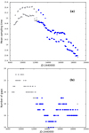 |
Fig. A.1. Variation in (panel a) mean sampling time and (panel b) number of gaps of the light curve over time. The gray dots represent the period from 1980–1990, and the blue dots show the period from 1990 onward. The oscillation in panel a is due to the periodic gaps that arise from lack of visibility of α-Orionis during part of the year. |
Appendix B: Construction of recurrence plots
In this appendix we briefly describe the construction process of recurrence plots (RPs) and discuss the parameters we used. The process consists of two steps: embedding, and calculating the recurrence matrix. The process of embedding leads to a reconstructed attractor (collection of trajectories) in the phase space where each point, or vector vi, represents a microstate. From the given time series yt, vectors vi are constructed as follows:
![Mathematical equation: $$ \begin{aligned} \boldsymbol{v}_{i} = [{ y}(t_{i}),{ y}(t_{i}+\tau ),{ y}(t_{i}+2\tau ),\ldots ,{ y}(t_{i}+(m-1)\tau )], \end{aligned} $$](/articles/aa/full_html/2020/08/aa38785-20/aa38785-20-eq1.gif) (B.1)
(B.1)
where m is the embedding dimension (dimension of the phase space), and τ is the delay (Takens 1981; Kantz & Schreiber 2004). Studies show that the properties of RPs do not vary significantly with embedding parameters (Thiel et al. 2004). We chose m = 1 and τ = 1.
When the vectors vi are known, the next step is to construct the recurrence matrix R as follows:
 (B.2)
(B.2)
where Θ is the Heaviside unit step function (Bracewell 2000),
 (B.3)
(B.3)
∥…∥ represent a distance norm (supremum norm used here) between vectors vi and vj, and ε is the distance threshold. The RP represents R visually, with zeros as white spaces and ones as black spaces. Structures formed by these recurrence points, such as the vertical lines, horizontal lines, and squares provide insight into the underlying dynamics. The distributions of these structures in the RP are quantified by the respective RQA measures, calculated from R (Marwan et al. 2002).
The RR is given as
 (B.4)
(B.4)
where N is the total number of points. We adopted a variable ε value for a fixed RR = 0.1.
Determinism, DET, captures the structure and extent of diagonal lines, indicating the degree to which we can predict the system:
 (B.5)
(B.5)
where l represents the length and P(l) the distribution of the diagonal lines in the RP.
Laminarity, LAM, captures the structure and extent of vertical lines, reflecting the laminar phases in the system. A laminar phase in the system represents a micro-regime where the system spends much time. It is given as
 (B.6)
(B.6)
where v represents the length and P(v) the distribution of the vertical lines in the RP.
Appendix C: Variation with window size
In this appendix, we consider the variation of standard early warning signals with changing window size. We varied the window sizes for a bin size 10 from 100 to 500 for the dataset from 1990 onward. The results are presented in Tables C.1 and C.2 for standard early-warning-signal measures and recurrence quantification measures, respectively. The Kendall-τ coefficients were calculated using the scipy package, and the corrected significance values were calculated using the pymannkendall package (Virtanen et al. 2020; Hussain & Mahmud 2019). The conclusions drawn in the main text of this paper hold in general for a range of window sizes.
Kendall-τ correlation coefficient (τK) and p-value before and after applying the corrected Mann-Kendall test (Hamed & Rao 1998) for the ACF, variance, and α from the detrended fluctation analysis.
Kendall-τ correlation coefficient (τK) and p-value before and after applying the corrected Mann-Kendall test (Hamed & Rao 1998) for the DET and LAM measures from the recurrence quantification analysis.
All Tables
Significant increases in early warning signals prior to the dimming event in Betelgeuse data.
Significant increases in RQA measures prior to the dimming event in Betelgeuse data.
Kendall-τ correlation coefficient (τK) and p-value before and after applying the corrected Mann-Kendall test (Hamed & Rao 1998) for the ACF, variance, and α from the detrended fluctation analysis.
Kendall-τ correlation coefficient (τK) and p-value before and after applying the corrected Mann-Kendall test (Hamed & Rao 1998) for the DET and LAM measures from the recurrence quantification analysis.
All Figures
|
Fig. 1. Variation in (panel a) autocorrelation at lag-1, (panel b) variance, and (panel c) spectral coefficient, α, calculated from detrended fluctuation analysis prior to the dimming event. The period from 1980–1990 is shown in gray, and the period from 1990 onward is shown in green. A visible rise can be seen leading towards the event. The calculated quantifier is plotted at the end time of the moving window. |
| In the text | |
|
Fig. 2. Recurrence plot of the time series of Betelgeuse. Upper panel: corresponding time series (in blue). The red part (dimming) was not included in the analysis. The parameters used are m = 1, τ = 1, and fixed RR = 0.1. |
| In the text | |
|
Fig. 3. Variation in RQA measures (panel a) DET and (panel b) LAM prior to the dimming event for fixed RR = 0.1. The red line indicates the 95% confidence level. The color code is similar to that in Fig. 1. The gray region refers to 1980–1990. |
| In the text | |
|
Fig. A.1. Variation in (panel a) mean sampling time and (panel b) number of gaps of the light curve over time. The gray dots represent the period from 1980–1990, and the blue dots show the period from 1990 onward. The oscillation in panel a is due to the periodic gaps that arise from lack of visibility of α-Orionis during part of the year. |
| In the text | |
Current usage metrics show cumulative count of Article Views (full-text article views including HTML views, PDF and ePub downloads, according to the available data) and Abstracts Views on Vision4Press platform.
Data correspond to usage on the plateform after 2015. The current usage metrics is available 48-96 hours after online publication and is updated daily on week days.
Initial download of the metrics may take a while.