| Issue |
A&A
Volume 640, August 2020
|
|
|---|---|---|
| Article Number | L4 | |
| Number of page(s) | 9 | |
| Section | Letters to the Editor | |
| DOI | https://doi.org/10.1051/0004-6361/202038423 | |
| Published online | 30 July 2020 | |
Letter to the Editor
3HSP J095507.9+355101: A flaring extreme blazar coincident in space and time with IceCube-200107A
1
Institute for Advanced Study, Technische Universität München, Lichtenbergstrasse 2a, 85748 Garching bei München, Germany
e-mail: This email address is being protected from spambots. You need JavaScript enabled to view it.
2
Associated to Agenzia Spaziale Italiana, ASI, Via del Politecnico s.n.c., 00133 Roma, Italy
3
ICRANet, Piazzale della Repubblica 10, 65122 Pescara, Italy
4
European Southern Observatory, Karl-Schwarzschild-Str. 2, 85748 Garching bei München, Germany
5
Associated to INAF – Osservatorio Astronomico di Roma, Via Frascati 33, 00040 Monteporzio Catone, Italy
6
Technische Universität München, Physik-Department, James-Frank-Str. 1, 85748 Garching bei München, Germany
7
Institutt for fysikk, NTNU, Trondheim, Norway
8
INAF – Osservatorio Astronomico di Roma, Via Frascati 33, 00040 Monteporzio Catone, Italy
9
INAF – IASF Milano, Via Corti 12, 20133 Milano, Italy
Received:
15
May
2020
Accepted:
5
July
2020
Abstract
The uncertainty region of the highly energetic neutrino IceCube200107A includes 3HSP J095507.9+355101 (z = 0.557), an extreme blazar, which was detected in a high, very hard, and variable X-ray state shortly after the neutrino arrival. Following a detailed multiwavelength investigation, we confirm that the source is a genuine BL Lac. This new detection differs from TXS 0506+056, which is thus far the first source associated with IceCube neutrinos, and is considered a “masquerading” BL Lac. As in the case of TXS 0506+056, 3HSP J095507.9+355101 is also way off the so-called blazar sequence. We consider 3HSP J095507.9+355101 a possible counterpart to the IceCube neutrino. Finally, we discuss some theoretical implications in terms of neutrino production.
Key words: neutrinos / radiation mechanisms: non-thermal / galaxies: active / gamma rays: galaxies / BL Lacertae objects: general
© ESO 2020
1. Introduction
The IceCube Neutrino Observatory at the South Pole1 has detected tens of high-energy neutrinos of likely astrophysical origin (e.g. IceCube Collaboration 2017a; Schneider 2020; Stettner 2020, and references therein). So far, only one astronomical object has been significantly associated (in space and time) with some of these neutrinos, that is the bright blazar TXS 0506+056 at z = 0.3365 (IceCube Collaboration 2018a,b; Padovani et al. 2018; Paiano et al. 2018). It is clear, however, that blazars cannot be responsible for the whole IceCube signal (see IceCube Collaboration 2017b; Aartsen et al. 2017). The case for some blazars being neutrino sources, however, is mounting. Several studies have reported hints of a correlation between blazars and the arrival direction of astrophysical neutrinos (e.g. Padovani & Resconi 2014; Padovani et al. 2016; Lucarelli et al. 2019 and references therein) and possibly of ultra high-energy cosmic rays (Resconi et al. 2017). Moreover, very recently some of the authors of this Letter (Giommi et al. 2020a) have extended the detailed dissection of the region around the IceCube-170922A event related to TXS 0506+056 carried out by Padovani et al. (2018) to all the 70 public IceCube high-energy neutrinos that are well reconstructed (so-called tracks) and off the Galactic plane. This resulted in a 3.23σ (post-trial) excess of IBLs2 and HBLs with a best fit of 15 ± 4 signal sources, while no excess was found for LBLs. Given that TXS 0506+056 is also a blazar of the IBL/HBL type (Padovani et al. 2019) this result, together with previous findings, consistently points to growing evidence for a connection between some IceCube neutrinos and IBL and HBL blazars. We report on 3HSP J095507.9+355101, an HBL within the error region of the IceCube track IceCube-200107A (see Fig. 1), which was found to exhibit an X-ray flare the day after the neutrino arrival. This source belongs to the third high-synchrotron peaked (3HSP) catalogue (Chang et al. 2019), which includes blazars with  Hz. Actually, with a catalogued synchrotron peak frequency of ∼5 × 10¹⁷ Hz, and a significantly higher value during the flare (Sect. 2.2), this source belongs to the rare class of extreme blazars (e.g. Biteau et al. 2020, and references therein). We also comment on the nature of the source and the theoretical implications in terms of neutrino production. We use a ΛCDM cosmology with H0 = 70 km s−1 Mpc−1, Ωm, 0 = 0.3, and ΩΛ, 0 = 0.7.
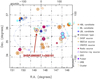 |
Fig. 1. Known and candidate blazars (radio/X-ray matching sources) around the 90% containment region of IceCube200107A, approximated by the elliptical area delimited by the dot-dashed curve. |
2. Multi-messenger data
2.1. IceCube data
On January 7, 2020 the IceCube Collaboration reported the detection of a high-energy neutrino candidate (HESE; Stein 2020) of possible astrophysical origin. While the event was not selected by the standard real-time detection procedure, it was identified as a starting track by a newly developed deep neural-network event classifier (Kronmueller & Glauch 2020). After applying off-line reconstructions, the arrival direction is given, as right ascension,  deg and declination
  deg at 90% C.L. As this was an unscheduled report, IceCube does not provide any energy information. Assuming an E−2 spectrum and the effective area for HESE starting tracks (IceCube Collaboration 2014), at this declination 90% of neutrinos have energy
  PeV3. Further evidence that the event is astrophysical comes from the direction. Because the event comes from the Northern Hemisphere, an atmospheric muon origin can be excluded. Also the fraction of the conventional atmospheric muon neutrino background is suppressed compared to the horizon. In a follow-up GCN report (Pizzuto 2020), IceCube announced the detection of two additional neutrino candidates in spatial coincidence with the 90% containment region of IceCube-200107A in a time range of two days around the alert consistent with atmospheric background at a 4% level. We note that the error region of IceCube-200107A is also fully inside the 16.5° median angular error circle of a HESE shower detected by IceCube in 2011 (HES9), and reported in IceCube Collaboration (2014). In fact, 3HSP J095507.9+355101 is located only 0.62° and 2.73° away from the best-fit position of IceCube-200107A and HES9, respectively.
We estimate the flux required to detect, on average, one muon neutrino with IceCube at a specified time interval, ΔT, by assuming the neutrino event, IceCube-200107A, to be a signal event. The number of signal-only, muon (and antimuon) neutrinos detected during ΔT at declination δ is given by  , where Eν, min and Eν, max, are the 90% C.L. lower and upper limits on the energy of the neutrino, respectively, Aeff is the effective area, and ϕEνμ the muon neutrino differential energy flux. We assume a source emitting an E−2 neutrino spectrum between 65 TeV and 2.6 PeV, the energy range in which we expect 90% of neutrinos detected from the direction of IC-200107A in the HESE channel. Since the neutrino emission duration is unknown we calculate the neutrino flux needed to produce one neutrino in IceCube from the direction of IceCube-200107A for ΔT = 30 d/250 d/10 yr, corresponding to the lower limit on the duration of the UV/soft X-ray flare (Sect. 2.2), the Fermi integration time (Sect. 2.4), and the duration of the IceCube operation, respectively. Using the effective area of Blaufuss et al. (2020), we obtain an integrated all-flavour neutrino energy flux of 3 × 10⁻⁹/4 × 10−10/3 × 10−11 erg cm−2 s−1, respectively, for a source at δ = 35.46°. This corresponds to energy-integrated, all-flavour neutrino luminosity, in the central 90% energy range, of ℒν ≈ 4 × 1048/5 × 1047/3 × 1046 erg s−1 for a source at z = 0.557. For a population of neutrino producing sources with summed expectation of order one neutrino, the energy flux estimate given above roughly corresponds to the total energy flux produced by the source population, whereas the individual source contribution, and thus the individual neutrino luminosity, is much lower than our estimate above (IceCube Collaboration 2018a).
2.2. Swift data
The Neil Gehrels Swift observatory (Gehrels et al. 2004) observed 3HSP J095507.9+355101 37 times; 26 pointings were performed between 2012 and 2013. The remaining pointings were carried out either as a Target of Opportunity (ToO) after the IceCube200107A event, which revealed the source to be in a flaring and very hard state (Giommi et al. 2020b; Krauss et al. 2020) or as part of a subsequent monitoring programme. We analysed all the X-Ray Telescope (XRT; Burrows et al. 2005) imaging data using Swift-DeepSky, a Docker container4 encapsulated pipeline software developed in the context of the Open Universe initiative (Giommi et al. 2018, 2019). Spectral analysis was also performed on all exposures with a sufficiently strong signal using the XSPEC-12 software embedded in a dedicated processing pipeline, called Swift-xrtproc, that was first presented in Giommi (2015). Details of the results are given in the appendix. The 2−10 keV emission from 3HSP J095507.9+355101 exhibited over a factor of ten variability in intensity associated with strong spectral changes following a harder-when-brighter trend (see Tables A.1, A.2, and Fig. A.1). The ToO observation of 3HSP J095507.9+355101 found this object in a flaring and hard state, with a 2−10 keV X-ray flux of ∼5 × 10⁻¹² erg cm−2 s−1 a factor 2.5 larger than the average value observed in 2012−2013, and with a power-law spectral index Γ = 1.8 ± 0.06. A log-parabola model gives a similar slope at 1 keV and curvature parameter consistent with zero, implying  Hz. The optical and UV data of the Ultra-Violet and Optical telescope (UVOT; Roming et al. 2005) were analysed using the on-line tools of the SSDC interactive archive5. Spectral data are shown in Fig. 2, while the X-ray light-curve is shown in Fig. 3. The optical/UV and low-energy X-ray data reach their maximum intensity after the neutrino arrival and remain approximately constant for the subsequent ∼30 days, implying that all the variability in the 2−10 keV band is induced by strong spectral changes above ∼7.3 × 10¹⁷ Hz.
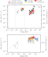 |
Fig. 2. 3HSP J095507.1+355101 SED. The grey points refer to archival data and, in the case of Fermi-LAT data, the time-integrated measurement up to the neutrino arrival alert. The average all-flavour neutrino flux is shown for an assumed live time of 10 yr. Coloured data points are Swift and NuSTAR measurements made around the neutrino arrival time. The black/grey γ-ray points refer to the red/grey bow ties, indicating the one-sigma uncertainty of the γ-ray measurement 250 days before the observation of IceCube-200107A and during the full mission, respectively. The best-fit fluxes are shown as solid lines. Upper panel: full hybrid SED, while lower panel: enlarged view of the optical and X-ray bands. |
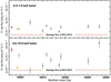 |
Fig. 3. Swift soft and hard X-ray monitoring of 3HSP J095507.1+355101 after the neutrino arrival. The first observation was carried out one day after the detection of IC200107A. The colours match those used in the SED of Fig. 2. The flux is higher than the average observed in 2012−2013 in both bands, but short-term variability is only present in the 2−10 KeV energy band. |
2.3. NuSTAR data
3HSP J095507.9+355101 was observed by the NuSTAR hard X-ray observatory (Harrison et al. 2013) four days after the detection of IceCube-200107A, following the results of the Swift ToO mentioned above. The observation was partly simultaneous with the third Swift pointing after the neutrino event. The source was detected between 3 keV and ∼30 keV. A power-law spectral fit gives a best-fit slope of Γ = 2.21 ± 0.06 with a reduced  = 0.93. The data, converted to spectral energy distribution (SED) units, are shown as light blue symbols in Fig. 2.
2.4. Fermi-LAT data
The analysis of the γ-ray emission of 3HSP J095507.9+355101 is based on publicly available Fermi-LAT Pass 8 data acquired in the period August 4, 2008 to January 8, 2020. In order to describe the spectral evolution of the source, we analysed two time windows: the full mission and the last 250 days before the detection of IceCube-200107A. The 250 days are needed to ensure the collection of sufficient photon statistics. The resulting fit between MJD 58605.6 and 58855.6 gives evidence for emission with significance of 2.9σ and spectral index of Γ = 1.73 ± 0.31 for a typical single power-law model. The spectral index over the full mission is Γ = 1.88 ± 0.15, with photon associations up to 178 GeV at 99% C.L. and a detection significance of 6.3σ. The corresponding photon fluxes integrated over the entire energy range between 100 MeV and the highest energy photon at 178 GeV are  ph cm−2 s−1 (250 days) and
  ph cm−2 s−1 (full mission), respectively. The best-fit spectra are also visualised together with their respective SED points in Fig. 2. More details on the data analysis are given in the appendix.
2.5. LBT data
3HSP J095507.9+355101 was observed on January 29, 2020 at the Large Binocular Telescope (LBT; Pogge et al. 2010) in the optical band (4100−8500 Å). A firm redshift z = 0.557 was derived thanks to the clear detection of absorption features attributed to its host galaxy. No narrow emission line was detected down to an equivalent width ∼0.3 Å. This corresponds to [O II] and [O III] line luminosities < 2 × 1040 erg s−1. Details about the spectroscopic study of the source, its host galaxy, and close environment are given in Paiano et al. (2020).
3. Nature of 3HSP J095507.9+355101
The SED of 3HSP J095507.9+355101, assembled using multi-frequency historical data, shows that this source exhibits a  Hz (Chang et al. 2019), which is a very large value that is rarely reached even by extreme blazars (Biteau et al. 2020). The 3HSP catalogue includes only 80 sources with
  Hz that have been detected by Fermi-LAT in ∼34 000 square degrees of high Galactic latitude sky (|b|> 10°), corresponding to an average density of one object every 425 square degrees. The chance probability that one such extreme source is included in the IC 200107A error region of 7.3 square degrees is therefore 7.3/425, or about 1.7%. At the time of the neutrino detection, 3HSP J095507.9+355101 was also found to be in a very hard state (
 Hz [10 keV] and flaring; see Fig. 2). Blazars are known to spend a small fraction of their time in a very high X-ray state (Giommi et al. 1990). We used the Open Universe blazar database (Giommi et al., in prep.) to estimate how frequently the extreme sources with
  Hz, and observed by Swift (in WT or PC mode; Burrows et al. 2005) more than 100 times (MRK421, MRK501, 1ES2344+514, and 1ES0033+595), are detected in a flaring state. We find that they spend less than 10% of the time at an intensity, that is larger than twice the average value. The overall chance probability of finding a blazar with
  as high as that of 3HSP J095507.9+355101 in the error region of IceCube-200107A during a flaring event is therefore a fraction of 1%. Since this is a posterior estimation based on archival data, which may hide possible biases, it should not be taken as evidence for a firm association, but rather as the identification of an uncommon and physically interesting event that corroborates a persistent trend (e.g. IceCube Collaboration 2018a; Giommi et al. 2020a) and motivates this work. We studied the nature of 3HSP J095507.1+355101, following Padovani et al. (2019), to check if this source is also a masquerading BL Lac like TXS 0506+056, that is intrinsically a flat-spectrum radio quasar (FSRQ) with the emission lines heavily diluted by a strong, Doppler-boosted jet. Given the upper limits on its LO II and LO III and its black hole mass estimate (MBH ∼ 3 × 10⁸ M⊙; Paiano et al. 2020), we obtained the following results for this source: 1. Its radio and O II luminosities put it at the very edge of the locus of jetted quasars (Fig. 4 of Kalfountzou et al. 2012). 2. Its Eddington ratio is L/LEdd < 0.02, which is formally still within the range of high-excitation galaxies (HEGs; characterised by L/LEdd ≳ 0.01) but barely so. 3. Its broad-line region (BLR) power in Eddington units is LBLR/LEdd < 3 × 10⁻⁴, which implies that this source is not an FSRQ according to Ghisellini et al. (2011) (as this would require LBLR/LEdd ≳ 5 × 10⁻⁴). 4. Finally, its Lγ/LEdd values range between ∼0.04 and ∼0.10, depending on its state, that is they straddle the BL Lac – FSRQ division proposed by Sbarrato et al. (2012) (Lγ/LEdd ∼ 0.1). Based on all of the above we consider 3HSP J095507.1+355101 an unlikely masquerading BL Lac. Figure 4 shows the location of 3HSP J095507.1+355101 on the
  versus Lγ plane in its average state and during the flare. The source is an extreme outlier of the so-called blazar sequence, even more so than TXS 0506+056. Given its Lγ, its
  should be about five orders of magnitude smaller to fit the sequence.
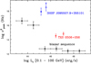 |
Fig. 4. Rest-frame |

4. Theoretical considerations and conclusions
We now present some general, model-independent, theoretical constraints on neutrino production by 3HSP J095507.9+355101 based on the multiwavelength observations. A comprehensive overview of models of neutrino emission from 3HSP J095507.9+355101 is presented in Petropoulou et al. (2020a). Neutrino production in the blazar jet is most likely facilitated by photo-pion (pπ) interactions. The neutrino production efficiency can thus be parametrised by fpπ, the optical depth to pπ interactions. Of the energy lost by protons with energy εp in pπ interactions, three-eighths go to neutrinos, resulting in the production of neutrinos with all-flavour luminosity, ενLεν = (3/8)fpπεpLεp. Each neutrino is produced with energy εν ≈ 0.05εp. Here and throughout, εLε is the luminosity per logarithmic energy, ε ⋅ dL/dε, unprimed symbols denote quantities in the cosmic rest frame, quantities with the subscript “obs” refer to the observer frame, and primed quantities refer to the frame co-moving with the jet. Neutrinos produced in interactions with photons co-moving with the jet have typical energy εν,obs ≈ 7.5 PeV(εt/2 keV)−1(Γ/20)2(1+z)−2, where Γ is the bulk Lorentz factor of the jet, and εt the energy of the target photons assuming that protons are accelerated to at least 150 PeV.
The remaining five-eighths of the proton energy lost go towards the production of electrons and pionic γ-rays. Synchrotron emission from electrons/positrons produced in pπ interactions and two-photon annihilation of the pionic γ-rays result in the synchrotron cascade flux (Murase et al. 2018) written as
 (1)
(1)
where YIC is the Compton-Y parameter, typically expected to be YIC ≪ 1 and the γ-ray emission is expected at energy  . The 250 day average luminosity of the flaring SED of 3HSP J095507.9+355101 in the Fermi-LAT energy range thus imposes a limit to the average neutrino luminosity according to Eq. (1). If the neutrino emission lasted 250 days, the expected neutrino luminosity of Eq. (1), is ∼2.2 orders of magnitude lower than the flux implied by the detection of one neutrino according to the estimate of Sect. 2.1, which is ενLεν = ℒν/ln(2.6 PeV/65 TeV) ≈ 1.3 × 1047 erg s−1. The expected neutrino luminosity as a function of the proton luminosity is shown in Fig. 5, for two characteristic values of fpπ (by definition fpπ ≤ 1), together with the constraint imposed by Eq. (1) and the luminosity needed to produce 1 neutrino in IceCube. Figure 5 also gives the “baryon loading” factor, ξ, implied by a given proton luminosity, defined in this work as ξ = εpLεp/εγLεγ6. Considering the long-term average Fermi-LAT flux instead, Eq. (1) leads to an upper limit on
 ![Mathematical equation: $ \varepsilon_{\nu} L_{\varepsilon_{\nu}} \approx [6 /(1+Y_{\mathrm{IC}})5]\varepsilon_{\gamma} L_{\varepsilon_{\gamma}}|_{\varepsilon^{\mathrm{p\pi}}_{\mathrm{syn}}} \approx 3 \times 10^{44} $](/articles/aa/full_html/2020/08/aa38423-20/aa38423-20-eq20.gif) erg s−1. This is a factor of ∼30 lower than the neutrino luminosity needed to detect 1 neutrino in IceCube, assuming a 10 yr live time, which is ℒν/ln(2.6 PeV/65 TeV) ≈ 8 × 1045 erg s−1. Thus, if the neutrino emission was related to the long-term emission of 3HSP J095507.9+355101, it is easier to satisfy the γ-ray emission constraint than if the neutrino emission was related to the Fermi-LAT 250-day high state. These results are also summarised in Fig. 5. Below the threshold for pπ interactions, protons lose energy via the Bethe-Heitler (BH) process. Unlike in the case of TXS 0506+056, for 3HSP J095507.9+355101 there are no observations available to constrain the BH cascade component and the most stringent constraint on the neutrino luminosity comes from the pπ cascade. Figure 5 reveals the difficulty of canonical theoretical models to explain the observation of one neutrino from 3HSP J095507.9+355101 during the 250 day Fermi high state, and to a lesser extent during the 10 yr of IceCube observations. The Poisson probability to detect one neutrino is ∼0.01 and ∼0.03 for the two timescales, respectively, which could be interpreted as a statistical fluctuation to account for the association. We note that a similar neutrino luminosity upper limit has been derived in one-zone models of neutrino production of TXS 0506+056 during its 2017 flare (Ansoldi et al. 2018; Cerruti et al. 2019; Gao et al. 2019; Keivani et al. 2018; Petropoulou et al. 2020b), which must also be interpreted as an upward (∼2σ) fluctuation to account for the observed association. On the other hand, Eq. (1) assumes that neutrinos and γ-rays are co-spatially emitted. In the presence of multiple emitting zones, and/or an obscuring medium for the γ-rays, the constraint of Eq. (1) can be relaxed and larger neutrino luminosity may be produced by 3HSP J095507.9+355101 (see for example such models for the 2017 flare of TXS 0506+056: Murase et al. 2018; Liu et al. 2019; Oikonomou et al. 2019; Xue et al. 2019; Zhang et al. 2020).
erg s−1. This is a factor of ∼30 lower than the neutrino luminosity needed to detect 1 neutrino in IceCube, assuming a 10 yr live time, which is ℒν/ln(2.6 PeV/65 TeV) ≈ 8 × 1045 erg s−1. Thus, if the neutrino emission was related to the long-term emission of 3HSP J095507.9+355101, it is easier to satisfy the γ-ray emission constraint than if the neutrino emission was related to the Fermi-LAT 250-day high state. These results are also summarised in Fig. 5. Below the threshold for pπ interactions, protons lose energy via the Bethe-Heitler (BH) process. Unlike in the case of TXS 0506+056, for 3HSP J095507.9+355101 there are no observations available to constrain the BH cascade component and the most stringent constraint on the neutrino luminosity comes from the pπ cascade. Figure 5 reveals the difficulty of canonical theoretical models to explain the observation of one neutrino from 3HSP J095507.9+355101 during the 250 day Fermi high state, and to a lesser extent during the 10 yr of IceCube observations. The Poisson probability to detect one neutrino is ∼0.01 and ∼0.03 for the two timescales, respectively, which could be interpreted as a statistical fluctuation to account for the association. We note that a similar neutrino luminosity upper limit has been derived in one-zone models of neutrino production of TXS 0506+056 during its 2017 flare (Ansoldi et al. 2018; Cerruti et al. 2019; Gao et al. 2019; Keivani et al. 2018; Petropoulou et al. 2020b), which must also be interpreted as an upward (∼2σ) fluctuation to account for the observed association. On the other hand, Eq. (1) assumes that neutrinos and γ-rays are co-spatially emitted. In the presence of multiple emitting zones, and/or an obscuring medium for the γ-rays, the constraint of Eq. (1) can be relaxed and larger neutrino luminosity may be produced by 3HSP J095507.9+355101 (see for example such models for the 2017 flare of TXS 0506+056: Murase et al. 2018; Liu et al. 2019; Oikonomou et al. 2019; Xue et al. 2019; Zhang et al. 2020).
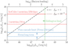 |
Fig. 5. All-flavour neutrino luminosity as a function of proton luminosity for two different values of the optical depth to photo-pion interactions fpπ. The red solid (dashed) line gives the neutrino luminosity corresponding to 1 muon neutrino in IceCube from 3HSP J095507.9+355101 if the neutrino emission lasted 250 days (10 yr). The blue horizontal solid (dashed) line gives the upper limit to the neutrino luminosity implied by the Fermi-LAT 250-day (long-term average) spectrum. The green line shows the upper limit to the proton luminosity implied by the Eddington luminosity of the 3 × 10⁸ M⊙ black hole, assuming Γ = 20, proton spectral index −2, and maximum proton energy 1018 eV. |
In summary, 3HSP J095507.9+355101, with its extremely high  is the second IBL/HBL that is off the blazar sequence to be detected in the error region of a high-energy neutrino during a flare. The Eddington ratio and upper limit to the BLR power we obtained make 3HSP J095507.9+355101 an unlikely masquerading BL Lac, in contrast to TXS 0506+056; this new observation points to a different class of possible neutrino-emitting BL Lac objects, which do not possess a (hidden) powerful BLR but have abundant > keV photons, owing to the high
  , which may facilitate PeV neutrino production. As was the case with TXS 0506+056, a possible association points to non-standard (“one-zone”) theoretical models, and/or the existence of an underlying population of sources each expected to produce ≪1 neutrinos in IceCube but with summed expectation ≥1. Figure 5 reveals that ∼150 (30) sources identical to 3HSP J095507.9+355101 are needed to produce one neutrino in 250 days (10 years), corresponding to an expectation of ≲0.01 neutrinos from a single blazar of this type. This would imply that the IceCube sensitivity is still above the expected fluxes from similar individual blazars, and the currently observed neutrino counting, if due to blazars, must be driven by large statistical fluctuations. A possible way to reconcile observations with expectations is to consider that there are about 100 catalogued blazars with properties similar to 3HSP J095507.1+355101. If each of these objects emits an average flux of ∼0.01 neutrinos in the period considered, we would be in a situation of extremely low counting statistics where the probability of observing one neutrino from a specific blazar is of the order of 1%. Collectively, however, one neutrino would be expected on similar timescales from one of the ∼100 randomly distributed blazars in the underlying population. This scenario is consistent with the current situation where only single neutrino events from each candidate counterparts are observed. Examples supporting this view are the extreme blazars 3HSP J023248.6+201717, 3HSP J144656.8−265658, and 3HSP J094620.2+010452, which are located inside the 90% uncertainty region of IC 111216A, IC 170506A, and IC 190819 (Giommi et al. 2020a).
Blazars are divided based on the rest-frame frequency of the low-energy (synchrotron) hump ( ) into LBL/LSP sources (
 Hz [< 0.41 eV]), intermediate- (1014 Hz <
  Hz [0.41 eV−4.1 eV]), and high-energy (
 Hz [> 4.1 eV]) peaked (IBL/ISP and HBL/HSP) sources, respectively (Padovani & Giommi 1995; Abdo et al. 2010).
For an assumed E−1/E−2.7 neutrino spectrum, 90% of neutrinos have energy  PeV /
PeV / PeV respectively.
We approximated εγLεγ ∼ ℒγ/ln(320 GeV/100 MeV), where ℒγ = 5.66 × 1045 erg s−1 is the γ-ray luminosity measured with the Fermi-LAT during the 250 day flare.
Acknowledgments
We acknowledge the use of data and software facilities from the ASI-SSDC and the tools developed within the United Nations “Open Universe” initiative. This work is supported by the Deutsche Forschungsgemeinschaft through grant SFB 1258 “Neutrinos and Dark Matter in Astro and Particle Physics”. We thank Riccardo Middei for his help with the analysis of NuSTAR data. We thank Matthias Huber and Michael Unger for useful discussions on the interpretation of the IceCube observations.
References
- Aartsen, M. G., Abraham, K., Ackermann, M., et al. 2017, ApJ, 835, 45 [NASA ADS] [CrossRef] [Google Scholar]
- Abdo, A. A., Ackermann, M., Agudo, I., et al. 2010, ApJ, 716, 30 [NASA ADS] [CrossRef] [Google Scholar]
- Ansoldi, S., Antonelli, L. A., Arcaro, C., et al. 2018, ApJ, 863, L10 [NASA ADS] [CrossRef] [Google Scholar]
- Biteau, J., Prandini, E., Costamante, L., et al. 2020, Nat. Astron., 4, 124 [CrossRef] [Google Scholar]
- Blaufuss, E., Kintscher, T., Lu, L., & Tung, C. F. 2020, PoS ICRC2019, 1021 [Google Scholar]
- Burrows, D. N., Hill, J. E., Nousek, J. A., et al. 2005, Space Sci. Rev., 120, 165 [NASA ADS] [CrossRef] [Google Scholar]
- Cerruti, M., Zech, A., Boisson, C., et al. 2019, MNRAS, 483, L12 [NASA ADS] [CrossRef] [Google Scholar]
- Chang, Y. L., Arsioli, B., Giommi, P., Padovani, P., & Brandt, C. H. 2019, A&A, 632, A77 [CrossRef] [EDP Sciences] [Google Scholar]
- Gao, S., Fedynitch, A., Winter, W., & Pohl, M. 2019, Nat. Astron., 3, 88 [NASA ADS] [CrossRef] [Google Scholar]
- Gehrels, N., Chincarini, G., Giommi, P., et al. 2004, ApJ, 611, 1005 [NASA ADS] [CrossRef] [Google Scholar]
- Ghisellini, G., Tavecchio, F., Foschini, L., & Ghirlanda, G. 2011, MNRAS, 414, 2674 [NASA ADS] [CrossRef] [Google Scholar]
- Ghisellini, G., Righi, C., Costamante, L., & Tavecchio, F. 2017, MNRAS, 469, 255 [NASA ADS] [CrossRef] [Google Scholar]
- Giommi, P. 2015, J. High Energy Astrophys., 7, 173 [NASA ADS] [CrossRef] [Google Scholar]
- Giommi, P., Barr, P., Garilli, B., Maccagni, D., & Pollock, A. M. T. 1990, ApJ, 356, 432 [NASA ADS] [CrossRef] [Google Scholar]
- Giommi, P., Arrigo, G., Barres De Almeida, U., et al. 2018, ArXiv e-prints [arXiv:1805.08505] [Google Scholar]
- Giommi, P., Brandt, C. H., Barres de Almeida, U., et al. 2019, A&A, 631, A116 [NASA ADS] [CrossRef] [EDP Sciences] [Google Scholar]
- Giommi, P., Glauch, T., Padovani, P., et al. 2020a, MNRAS, in press [arXiv:2001.09355] [Google Scholar]
- Giommi, P., Glauch, T., & Resconi, E. 2020b, ATel, 13394, 1 [Google Scholar]
- Harrison, F. A., Craig, W. W., Christensen, F. E., et al. 2013, ApJ, 770, 103 [NASA ADS] [CrossRef] [Google Scholar]
- IceCube Collaboration 2014, Phys. Rev. Lett., 113, 101101 [NASA ADS] [CrossRef] [PubMed] [Google Scholar]
- IceCube Collaboration 2017a, ArXiv e-prints [arXiv:1710.01191] [Google Scholar]
- IceCube Collaboration 2017b, ArXiv e-prints [arXiv:1710.01179] [Google Scholar]
- IceCube Collaboration 2018a, Science, 361, eaat1378 [CrossRef] [Google Scholar]
- IceCube Collaboration 2018b, Science, 361, 147 [CrossRef] [Google Scholar]
- Kalfountzou, E., Jarvis, M. J., Bonfield, D. G., & Hardcastle, M. J. 2012, MNRAS, 427, 2401 [NASA ADS] [CrossRef] [Google Scholar]
- Keivani, A., Murase, K., Petropoulou, M., et al. 2018, ApJ, 864, 84 [NASA ADS] [CrossRef] [Google Scholar]
- Krauss, F., Gregoire, T., Fox, D. B., Kennea, J., & Evans, P. 2020, ATel, 13395, 1 [Google Scholar]
- Kronmueller, M., & Glauch, T. 2020, PoS ICRC2019, 937 [Google Scholar]
- Liu, R.-Y., Wang, K., Xue, R., et al. 2019, Phys. Rev. D, 99, 063008 [NASA ADS] [CrossRef] [Google Scholar]
- Lucarelli, F., Tavani, M., Piano, G., et al. 2019, ApJ, 870, 136 [CrossRef] [Google Scholar]
- Massaro, E., Perri, M., Giommi, P., & Nesci, R. 2004, A&A, 413, 489 [NASA ADS] [CrossRef] [EDP Sciences] [Google Scholar]
- Murase, K., Oikonomou, F., & Petropoulou, M. 2018, ApJ, 865, 124 [NASA ADS] [CrossRef] [EDP Sciences] [Google Scholar]
- Oikonomou, F., Murase, K., Padovani, P., Resconi, E., & Mészáros, P. 2019, MNRAS, 489, 4347 [CrossRef] [Google Scholar]
- Padovani, P., & Giommi, P. 1995, ApJ, 444, 567 [NASA ADS] [CrossRef] [Google Scholar]
- Padovani, P., & Resconi, E. 2014, MNRAS, 443, 474 [NASA ADS] [CrossRef] [Google Scholar]
- Padovani, P., Resconi, E., Giommi, P., Arsioli, B., & Chang, Y. L. 2016, MNRAS, 457, 3582 [NASA ADS] [CrossRef] [Google Scholar]
- Padovani, P., Giommi, P., Resconi, E., et al. 2018, MNRAS, 480, 192 [NASA ADS] [CrossRef] [Google Scholar]
- Padovani, P., Oikonomou, F., Petropoulou, M., Giommi, P., & Resconi, E. 2019, MNRAS, 484, L104 [NASA ADS] [CrossRef] [Google Scholar]
- Paiano, S., Falomo, R., Treves, A., & Scarpa, R. 2018, ApJ, 854, L32 [NASA ADS] [CrossRef] [Google Scholar]
- Paiano, S., Falomo, R., Padovani, P., et al. 2020, MNRAS, 495, L108 [CrossRef] [Google Scholar]
- Petropoulou, M., Oikonomou, F., Mastichiadis, A., et al. 2020a, ApJ, submitted [arXiv:2005.07218] [Google Scholar]
- Petropoulou, M., Murase, K., Santander, M., et al. 2020b, ApJ, 891, 115 [CrossRef] [Google Scholar]
- Pizzuto, A. 2020, GRB Coordinates Network, 26704, 1 [Google Scholar]
- Pogge, R. W., Atwood, B., Brewer, D. F., et al. 2010, Proc. SPIE, 7735, 77350A [CrossRef] [Google Scholar]
- Resconi, E., Coenders, S., Padovani, P., Giommi, P., & Caccianiga, L. 2017, MNRAS, 468, 597 [NASA ADS] [CrossRef] [Google Scholar]
- Roming, P. W. A., Kennedy, T. E., Mason, K. O., et al. 2005, Space Sci. Rev., 120, 95 [NASA ADS] [CrossRef] [Google Scholar]
- Sbarrato, T., Ghisellini, G., Maraschi, L., & Colpi, M. 2012, MNRAS, 421, 1764 [NASA ADS] [CrossRef] [Google Scholar]
- Schneider, A. 2020, PoS ICRC2019, 1004 [Google Scholar]
- Stein, R. 2020, GRB Coordinates Network, 26655, 1 [Google Scholar]
- Stettner, J. 2020, PoS ICRC2019, 1017 [Google Scholar]
- Xue, R., Liu, R.-Y., Petropoulou, M., et al. 2019, ApJ, 886, 23 [NASA ADS] [CrossRef] [Google Scholar]
- Zhang, B. T., Petropoulou, M., Murase, K., & Oikonomou, F. 2020, ApJ, 889, 118 [CrossRef] [Google Scholar]
Appendix A
In this appendix we give details of the multi-frequency data analysis of 3HSP J095507.1+355101.
A.1. Swift-XRT
All Swift-XRT observations were analysed using Swift-DeepSky and Swift-xrtproc, the imaging and spectral analysis tools developed within the Open Universe initiative (Giommi et al. 2019; Giommi 2015). Both tools are based on the official HEASoft data reduction package, in particular on XIMAGE-4.5 and XSPEC-12; these tools are particularly useful when analysing a large number of observations, as the tools automatically download the data and calibration files from one of the official archives, generate all the necessary intermediate products, and conduct a detailed standard analysis. The results of the image analysis are presented in Table A.1, in which Col. 1 gives the observation start time, Col. 2 gives the effective exposure time, Col. 3 gives the count rate in the 0.3−10 keV band, and Cols. 4–7 give the flux in the 0.3−10, 0.3−1.0, 1−2 keV, and 2−10 KeV bands, respectively. The largest flux variations are observed in the 2−10 keV band where the intensity varied by over a factor ten, between a minimum of 0.55 × 10⁻¹² erg cm−2 s−1 on MJD 56233 (Nov. 2, 2012) and a maximum of 6.16 × 10⁻¹² erg cm−2 s−1 on MJD 58900 (Feb. 21, 2020).
Results of the imaging analysis of all Swift-XRT observations of 3HSP J095507.1+355101 with exposure time larger than 200 s.
Details of the spectral analysis for the cases of power-law and log parabola models with NH fixed to the Galactic value, are given in Table A.2. Column 1 gives the observation date, Col. 2 gives the best fit photon spectral index with one σ error, Col. 3 gives the value of the reduced χ2 with the number of degrees of freedom (d.o.f.) in parenthesis, Cols. 4 and 5 give the spectral slope at 1 keV (α) and curvature parameter (β) with one σ error, and Col. 6 the corresponding reduced χ2 and d.o.f. Figure A.1 shows the best-fit power-law spectral index versus the 2−10 keV flux, for all the observations where the error on the spectral slope is smaller than 0.25. The figure shows a clear harder-when-brighter trend, a behaviour seen in several other HBL blazars (e.g. Giommi et al. 1990).
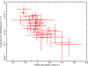 |
Fig. A.1. Best-fit power-law spectral index of all the observations with errors smaller than 0.25 is plotted vs. the 2−10 keV X-ray flux of 3HSP J095507.1+355101. |
Results of the spectral analysis of all Swift-XRT observations of 3HSP J095507.1+355101 with at least 25 net counts.
A.2. NuSTAR
Data from the NuSTAR observation made shortly after the neutrino arrival were analysed using the XSPEC12 package. Photons detected by both telescopes (module A and B) were combined and fitted to spectral models following the standard XSPEC procedure. The source was detected between 3 keV and 30 keV. A power-law spectral model gives a best-fit slope of Γ = 2.21 ± 0.06 with a reduced  = 0.93 with 101 d.o.f. A fit to a log parabola model does not improve the reduced
  and therefore it is not reported here. A combined fit of the NuSTAR and the quasi-simultaneous Swift-XRT data with a log parabola model gives the following best-fit parameters: α = 1.80 ± 0.07, β = 0.24 ± 0.05 for a pivot energy Epivot = 1 keV, and reduced
  = 0.86 with 129 d.o.f. The corresponding SED peak energy, estimated as Epeak = 10(2 − α)/2β (Massaro et al. 2004), is Epeak ∼ 2.6 keV.
A.3. Fermi
For the analysis of the γ-ray emission of 3HSP J095507.9+355101 we used the publicly available Fermi-LAT Pass 8 data acquired in the period August 4, 2008 to January 8, 2020 and followed the standard procedure as described in the Fermi cicerone7. We constructed a model that contains all known 4FGL sources plus the diffuse Galactic and isotropic emissions. In the likelihood fits, we left free the normalisation and spectral index of all sources within 10° (corresponding to the 95% Fermi point-spread function at 100 MeV). To calculate an a priori estimate of the required integration time for a significant detection of the source, we used the time-integrated measurement in the Fermi 4FGL catalogue. Assuming a signal dominated counting experiment with  background test-statistic distribution we know that the median test statistic distribution scales linearly in time t, i.e., 𝒯𝒮 ∝ t and, therefore,
![Mathematical equation: $$ \begin{aligned} t_{\rm lc} = ({\mathcal{TS} }_{\rm lc}/{\mathcal{TS} }_{\rm 2920d})\cdot 2920 \, [\mathrm{days}] , \end{aligned} $$](/articles/aa/full_html/2020/08/aa38423-20/aa38423-20-eq33.gif) (A.1)
(A.1)
assuming a quasi-steady emission. Here 𝒯𝒮lc defines the target test-statistic value with required integration time tlc. 2920 days and 𝒯𝒮2920d are the live time and significance of the source in the 4FGL catalogue, respectively. We note that in general for the significance  . The source is detected with a significance of 5.42σ in the 4FGL catalogue and hence the resulting integration times for one and two sigma are 100 days and 400 days, respectively. In order to avoid washing out a possible time-dependent signal we chose an integration time of 250 days. Table A.3 gives the significance of all γ-ray data points shown in the SED in Fig. 2.
Energy dependent significance of the Fermi-LAT SED for the full-mission and the 250 days before the neutrino alert.
All Tables
Results of the imaging analysis of all Swift-XRT observations of 3HSP J095507.1+355101 with exposure time larger than 200 s.
Results of the spectral analysis of all Swift-XRT observations of 3HSP J095507.1+355101 with at least 25 net counts.
Energy dependent significance of the Fermi-LAT SED for the full-mission and the 250 days before the neutrino alert.
All Figures
|
Fig. 1. Known and candidate blazars (radio/X-ray matching sources) around the 90% containment region of IceCube200107A, approximated by the elliptical area delimited by the dot-dashed curve. |
| In the text | |
|
Fig. 2. 3HSP J095507.1+355101 SED. The grey points refer to archival data and, in the case of Fermi-LAT data, the time-integrated measurement up to the neutrino arrival alert. The average all-flavour neutrino flux is shown for an assumed live time of 10 yr. Coloured data points are Swift and NuSTAR measurements made around the neutrino arrival time. The black/grey γ-ray points refer to the red/grey bow ties, indicating the one-sigma uncertainty of the γ-ray measurement 250 days before the observation of IceCube-200107A and during the full mission, respectively. The best-fit fluxes are shown as solid lines. Upper panel: full hybrid SED, while lower panel: enlarged view of the optical and X-ray bands. |
| In the text | |
|
Fig. 3. Swift soft and hard X-ray monitoring of 3HSP J095507.1+355101 after the neutrino arrival. The first observation was carried out one day after the detection of IC200107A. The colours match those used in the SED of Fig. 2. The flux is higher than the average observed in 2012−2013 in both bands, but short-term variability is only present in the 2−10 KeV energy band. |
| In the text | |
|
Fig. 4. Rest-frame |
| In the text | |
|
Fig. 5. All-flavour neutrino luminosity as a function of proton luminosity for two different values of the optical depth to photo-pion interactions fpπ. The red solid (dashed) line gives the neutrino luminosity corresponding to 1 muon neutrino in IceCube from 3HSP J095507.9+355101 if the neutrino emission lasted 250 days (10 yr). The blue horizontal solid (dashed) line gives the upper limit to the neutrino luminosity implied by the Fermi-LAT 250-day (long-term average) spectrum. The green line shows the upper limit to the proton luminosity implied by the Eddington luminosity of the 3 × 10⁸ M⊙ black hole, assuming Γ = 20, proton spectral index −2, and maximum proton energy 1018 eV. |
| In the text | |
|
Fig. A.1. Best-fit power-law spectral index of all the observations with errors smaller than 0.25 is plotted vs. the 2−10 keV X-ray flux of 3HSP J095507.1+355101. |
| In the text | |
Current usage metrics show cumulative count of Article Views (full-text article views including HTML views, PDF and ePub downloads, according to the available data) and Abstracts Views on Vision4Press platform.
Data correspond to usage on the plateform after 2015. The current usage metrics is available 48-96 hours after online publication and is updated daily on week days.
Initial download of the metrics may take a while.