| Issue |
A&A
Volume 640, August 2020
|
|
|---|---|---|
| Article Number | A45 | |
| Number of page(s) | 10 | |
| Section | The Sun and the Heliosphere | |
| DOI | https://doi.org/10.1051/0004-6361/202038141 | |
| Published online | 10 August 2020 | |
Inference of chromospheric plasma parameters on the Sun
Multilayer spectral inversion of strong absorption lines
Astronomy Program, Department of Physics and Astronomy, Seoul National University, Seoul, 08826, Korea
e-mail: This email address is being protected from spambots. You need JavaScript enabled to view it.
Received:
10
April
2020
Accepted:
9
June
2020
Abstract
The solar chromosphere can be observed well through strong absorption lines. We infer the physical parameters of chromospheric plasmas from these lines using a multilayer spectral inversion. This is a new technique of spectral inversion. We assume that the atmosphere consists of a finite number of layers. In each layer the absorption profile is constant and the source function varies with optical depth with a constant gradient. Specifically, we consider a three-layer model of radiative transfer where the lowest layer is identified with the photosphere and the two upper layers are identified with the chromosphere. The absorption profile in the photosphere is described by a Voigt function, and the profile in the chromosphere by a Gaussian function. This three-layer model is fully specified by 13 parameters. Four parameters can be fixed to prescribed values, and one parameter can be determined from the analysis of a satellite photospheric line. The remaining 8 parameters are determined from a constrained least-squares fitting. We applied the multilayer spectral inversion to the spectral data of the Hα and the Ca II 854.21 nm lines taken in a quiet region by the Fast Imaging Solar Spectrograph (FISS) of the Goode Solar Telescope (GST). We find that our model successfully fits most of the observed profiles and produces regular maps of the model parameters. The combination of the inferred Doppler widths of the two lines yields reasonable estimates of temperature and nonthermal speed in the chromosphere. We conclude that our multilayer inversion is useful to infer chromospheric plasma parameters on the Sun.
Key words: Sun: atmosphere / Sun: photosphere / Sun: chromosphere / methods: data analysis / radiative transfer / line: profiles
© ESO 2020
1. Introduction
Strong absorption lines in the visible and infrared wavelengths are important spectral windows into the solar chromosphere. These lines are observable from the ground and contain useful information of chromospheric plasmas. The Hα line of hydrogen has been the most popular of these windows. This line is favored because it is strong, and broad enough for filtergraph observations. The Hα filter images of solar regions display a great variety of intensity structures (Rutten 2008; Leenaarts et al. 2012). Even though the image data of the intensity directly provide much useful (mostly morphological) information of the underlying plasma structures, they do not provide estimates of plasma parameters, which are crucial for understanding the physical conditions. The inference of plasma parameters requires the spectral data of the strong absorption lines and a successful spectral inversion.
Spectral inversion is the process of inferring the plasma parameters from the observed profile of a spectral line. Two types of spectral inversion have been popular in solar observations that assume the constancy of physical parameters. One is the Milne-Eddington inversion, and the other is the cloud model inversion (Beckers 1964). The Milne-Eddington inversion is based on the assumption that the spectral line is formed in a plasma layer of infinite optical thickness where the absorption profile is constant over optical depth and the source function varies with a constant gradient. This inversion has been used mainly to model spectral lines formed in the photosphere and to infer the magnetic fields from their Stokes profiles (Unno 1956; Skumanich & Lites 1987).
The cloud model inversion, on the other hand, assumes that the line is formed in a plasma layer of finite optical depth where the source function as well as the absorption profile is constant over optical depth. This model has been used mostly to infer the physical parameters of cloud-like features lying far above the solar surface (Tziotziou 2007), as was well illustrated in Fig. 1 of Heinzel et al. (1999). A number of variants have been proposed to generalize the original cloud model of Beckers (1964) by incorporating the varying source function (Mein et al. 1996; Heinzel et al. 1999; Tsiropoula et al. 1999), the presence of multiple clouds (Gu et al. 1996), the concept of the embedded cloud (Steinitz et al. 1977; Chae 2014), etc. Despite these variants, the usage of the cloud model inversion is still limited, and is often hampered by the difficulty of choosing the incident intensity profile. Because the incident intensity below the feature of interest cannot be determined from observations, it has to be assumed to be the same as that in its neighborhood, for instance.
Here we present a multilayer inversion for modeling the spectral profiles of strong absorption lines. This represents a combined generalization of the two types of spectral inversion. A strong line is formed over a wide height range of the atmosphere from the photosphere to the chromosphere. The formation of the line in the photosphere can be modeled by the Milne-Eddington model, and the formation in the chromosphere can be modeled by the cloud model inversion. When the source function is allowed to vary with optical depth, there is no fundamental difference between the two types of inversion. Thus we expect that the formation of a strong line can be modeled by the radiative transfer across a finite number of layers in each of which the absorption profile is constant and the source function varies with a constant gradient over optical depth. This is the multilayer inversion we aim to implement.
In this multilayer inversion, parameters other than the source function are kept constant in each layer, but they can vary from layer to layer throughout the solar atmosphere. In this regard, the multilayer inversion method is somewhat similar to the response-function-based inversion proposed by Ruiz Cobo & del Toro Iniesta (1992, 1994) to infer height-varying temperature, magnetic field, and line-of-sight velocity from Stokes profiles.
The multilayer spectral inversion is described in detail in the following section. Its specific version, the three-layer model, is applied to the spectral data of the Hα and Ca II 854.21 nm lines taken by the Fast Imaging Solar Spectrograph (FISS) of the Goode Solar Telescope (GST). We measure wavelengths in nm and pm, and lengths or distances on the Sun in km and Mm: 1 nm = 10−9 m = 10 Å, 1 pm = 10−3 nm = 10−2 Å = 10 mÅ, 1 km = 103 m, and 1 Mm = 106 m.
2. Multilayer spectral inversion
2.1. Multilayer model of radiative transfer
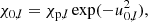
We assume that the source function S is independent of wavelength over the spectral line, and is given as a function of height in the atmosphere, which is measured by the optical depth tλ at a wavelength λ. If S is known as a function of tλ, the intensity emergent out of the atmosphere Iλ is given by the solution of the radiative transfer equation,
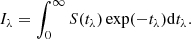 (1)
(1)
The atmosphere consists of the chromospheric layer of finite optical thickness τ0 at the line center and the photospheric layer of infinite optical thickness, therefore we can rewrite Eq. (1) as
 (2)
(2)
in terms of the chromospheric contribution Iλ, c and the photospheric contribution Iλ, p defined by
Here the operator L(t1, t2) is defined as
 (3)
(3)
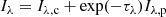
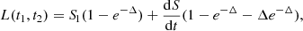
We can decompose the chromosphere into N layers of equal optical thickness δ0 = τ0/N at the line center (as illustrated in Fig. 1 in the case N = 2). Then we obtain the expression
 (4)
(4)
where
 (5)
(5)
which assumes constancy of rλ ≡ χλ/χ0 over optical depth in each layer, where χλ is the absorption coefficient at wavelength λ and χ0 is the absorption coefficient at the central wavelength λ0 of the line. The optical thickness of the chromospheric layer is then given by
 (6)
(6)
 |
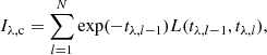
Fig. 1. Three-layer model of radiative transfer that consists of two chromospheric layers and one photospheric layer. |
We assume that the source function has a constant gradient dS/dt in each layer. Then the integration yields the expression
 (7)
(7)
written in terms of the source function at top S1 and Δ = t2 − t1.
In the chromospheric layers, the optical thickness is finite, therefore the gradient can be written in terms of the source function at the top Sl − 1, and the one Sl at the bottom of each layer indexed by l, and it follows
 (8)
(8)
with Δ = rλ, lδ0.
The absorption profile is assumed to be constant in each layer. In a chromospheric layer, the values of the line-of-sight velocity vl (defined to be positive in downward motion) and Doppler width wl are assumed to be constant over optical depth. The damping parameter and continuum absorption are set to zero. The absorption coefficient in the lth layer is described by the Gaussian function
 (9)
(9)
with the peak absorption coefficient χp, l, and
 (10)
(10)
The absorption profile at wavelength λ0 is given by
 (11)
(11)
with
 (12)
(12)
and we obtain
 (13)
(13)
In the photosphere, Δ is infinite in Eq. (7), and the gradient can be expressed as
 (14)
(14)
where tc is the continuum optical depth and Sp is the source function at the level of tc = 1. Thus Eq. (7) leads to the expression
 (15)
(15)
in the photosphere, where SN is the source function at the bottom of the lowest layer indexed by N.
The absorption profile is constant over depth in the photosphere as well. Here the continuum absorption is not negligible and the collisional broadening also has to be taken into account. The ratio of line center-to-continuum absorption η as well as the dimensionless damping parameter a is taken to be constant over optical depth. The absorption coefficient in the photosphere is then given by
 (16)
(16)
where χp, p is the peak absorption coefficient in the photosphere, and H is the Voigt function normalized to satisfy H(0, a)=1 with
 (17)
(17)
Thus we have
 (18)
(18)
with the line center-to-continuum opacity ratio η ≡ χp, p/χc.
In this work, we specifically consider the three-layer model of radiative transfer where the chromosphere is assumed to consist of two layers (N = 2), as illustrated in Fig. 1. We are mainly interested in the chromosphere. Because it covers a wide range of heights over which the physical conditions vary, it is necessary to describe it with a model of at least two layers. The three-layer model is the simplest model that includes the photospheric layer and characterizes both the height variation of the absorption profile and the nonlinear variation of the source function inside the chromosphere.
This model is fully specified by a total of 13 parameters. The optical thickness of the chromosphere is specified by τ0. The variation in source function is specified by the four parameters S0, S1, S2, and Sp, and the absorption profile is described by vp, wp, a, and η in the photosphere, by v2 and w2 in the lower chromosphere, and by v1 and w1 in the upper chromosphere.
2.2. Model fitting
We fit each profile of a strong absorption line with the model specified by the independent parameter vector, which is defined as
 (19)
(19)
where each element has a real value and log refers to the common logarithm to the base of 10. The adoption of the logarithmic values at the model parameters automatically guarantees the positivity requirement for η, wp, a, Sp, S2, τ0, w2, w1, S1, and S0.
For the regularized model fitting, we employ the technique of constrained least-squares fitting that minimizes the functional
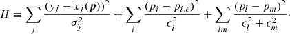 (20)
(20)
Here the first sum is the classical χ2 term where yj is the data, σy is the standard noise of data, and xj is the model with parameters pi. The second sum is the constraint on the individual components pi, where pi, e and ϵi are the expectation value of pi and its standard deviation, respectively, that are to be known from the a priori information. The third sum is the similarity constraint forcing absorption profiles in the two chromospheric layers to be similar to each other as far as the data allow. Specifically, we select (pl, pm)=(v1, v2), (logw1, logw2), and (logS, logS0).
Depending on the value of ϵi, the parameter pi can be categorized as either fixed or free. If ϵi is set to be very small, pi is practically fixed to pi, e. The value of vp is inferred from the center of the Ti II 655.958 nm line in the Hα band and the Si I 853.6165 nm line in the Ca II band. It is thus given as an input, and treated as a fixed parameter in the model fitting. In addition, we found after several experiments that most line profiles can be fairly well fit with logη, logwp, a, and τ0 being fixed to the values listed in Table 1.
Fixed parameters and their values.
We fix the values of logη, logwp, and a, because this reduces the degree of freedom and facilitates fitting the portions of the line profile that is formed in the photosphere. We also fix the value of τ0 because it is not uniquely determined from the fitting. We have examined the performance of the fitting by varying τ0. As a result, we found that in both lines, the fitting is fairly good, regardless of τ0, because it varies from 1 to 10. The fit becomes worse when τ0 becomes larger. Thus we fix τ0 to 10, the highest value that can yield a sufficiently good fitting.
There remain eight free parameters that have to be determined from the fitting itself. To determine these values, we first apply the fit to a large number of data sets without constraints (by setting ϵi = ∞). Then all p obtained with the best fit form an ensemble of p. The mean of pi over this ensemble is then identified with pi, e. The value of ϵi is set to the standard deviation of pi in the ensemble or, if necessary, to a higher value. The values of pi, e and ϵi are listed in Table 2.
Values of pi, e ± ϵi of the free parameters.
All the fits are made with respect to the clean wavelengths, that is, the wavelengths where the blending by other lines is negligible. We apply the fitting in two stages. In the first stage, the far wings of the line profile (with wavelength offsets larger than 1.2 Å in the Hα line and 0.8 Å in the Ca II line) are fit by the model
 (21)
(21)
assuming τλ is negligibly small. This first fitting produces the estimates of two parameters logSp and logS2, and the construction of Iλ, p over the whole line. With Iλ, p being determined, we can construct the contrast profile,
 (22)
(22)
This contrast profile is fit by the corresponding model at the clean wavelengths. This second fitting yields the estimates of the other six parameters: v2, v1, logw2, logw1, logS1, and logS0. The special condition of v2 = v1, w1, and S2 = S1 = S0 ≡ S reduces the above equation to that of the classical cloud model.
The goodness of fit is measured by the standard error ϵ defined by the root mean square of the difference between the observed Cλ and the model Cλ, where the average is taken over the clean wavelengths where the fitting is applied.
3. Data and reduction
3.1. Data
We used the spectral data taken with the FISS of the GST at Big Bear Solar Observatory (Chae et al. 2013). The FISS is a dual-band echelle spectrograph that usually records the Hα band and the Ca II 854.2 nm band simultaneously using two cameras. The cameras record the spectral ranges of 0.97 nm (Hα) and 1.29 nm (Ca II) with a pixel sampling of 1.9 pm and 2.5 pm, respectively. With a slit width of 0.16′′, the spectral resolving power (λ/δλ) is estimated at 140 000 and 130 000. We use the PCA-compressed spectral data where noise is suppressed very well (Chae et al. 2013). The signal-to-noise ratio of the compressed intensity data is 700 (Hα) and 250 (Ca II) at the line centers. The height of 40′′ is covered with the sampling of 0.16′′. The two-dimensional imaging of the FISS is achieved by scanning the slit across the field of view with a step size of 0.16′′.
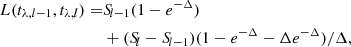
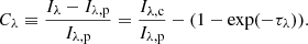
Figure 2 presents the monochromatic images of an observed region constructed from the raster-scan observation of a quiet-Sun region outside active regions. The time of observation was 17:14:06 UT on 2017 June 14. The field of view is 24′′ × 40′′ or 17.4 Mm × 29 Mm. Even though small, the field of view includes both network features and intranetwork features.
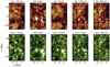 |
Fig. 2. Monochromatic images of a quiet region constructed at ten selected wavelengths. The two symbols mark the position of a intranetwork feature (x) and a network feature (+) selected for the illustration of the observed line profiles and the model fitting. |
3.2. Reduction
The average spectral profile of an observed solar region was taken as the reference profile. All the profiles were normalized by the maximum intensity (a proxy of the continuum intensity) of this reference profile. Each profile was then corrected for stray light in two steps following Chae et al. (2013). The observed line profile was corrected for spatial stray light by subtracting 0.027 times the reference profile from it and by then dividing it by 0.973. The corrected line profile was then corrected for spectral stray light by subtracting 0.065 times the maximum value of the line profile from it and by dividing it by 0.935.
The reference profile was also used to calibrate the wavelength precisely. In the Hα band, the centers of the Hα line and the Ti II 655.9580 nm line in the reference profile were determined in pixel units and were used to convert the wavelength pixels into physical wavelength values. In the Ca II band, the Ca II line itself could not be used as a reference because the center of this line averaged over a solar region is known to be offset from its laboratory wavelength. Instead, we used the pair of the Fe I 853.80152 nm line and the Si I 853.6165 nm line for the wavelength calibration. Thus the Doppler shift in each band was measured with respect to the average photosphere of the observed region.
Before applying the model fitting, we corrected each observed line profile for the slightly nonuniform pattern that may exist and may cause the asymmetry between the far blue wing and the far red wing. We fit the intensities at the far red and blue wings > 0.4 nm by a first-order polynomial. This fit, after normalizing by its mean value, was used as the estimate of the nonuniform pattern. The profile corrected for this pattern then had the required symmetry.
The observed spectral profiles of the Hα and the Ca II lines are contaminated by weak spectral lines in the same band, some of which are solar lines and others are terrestrial lines (mostly H2O lines). Fortunately, the terrestrial lines in our data are very weak, because the observatory is located in a dry land. The model fitting described below uses only the spectral data that are less contaminated by these satellite lines.
4. Results
4.1. Model fitting of line profiles
We applied the multilayer fitting to the profiles of the Hα and Ca II 854.2 nm lines. It took 0.018 s on average to fit each Hα line profile, and 0.046 s to fit each Ca II line profile when we used the Python 3.7 software installed on a laptop computer with a 1.80 GHz CPU and Windows 10 operating system.
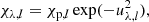
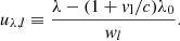
We found that the multilayer model fitting is reasonably good in both lines. The fitting of the line profiles of an intranetwork (IN) feature is illustrated in Fig. 3, and that of a network (NW) feature in Fig. 4. The standard error of the fitting is ϵ = 0.007 (IN) and 0.007 (NW) in the Hα line, and 0.013 (IN) and 0.006 (NW) in the Ca II line. The two figures show that the NW feature is different from the IN feature in the spectral characteristics. The NW feature has a broader profile of the Hα line and a higher core intensity of the Ca II line than the IN feature. For this reason, the model fitting produces a larger w1 of the Hα line and a higher S0 of the Ca II line in the NW feature than in the IN feature.
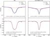 |
Fig. 3. Three-layer model fitting of the line profiles taken from an intranetwork feature marked by the cross in Fig. 2. The reference profile is the average of all the profiles over the observed region. |
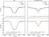 |
Fig. 4. Three-layer model fitting of the line profiles taken from a network feature marked by a plus in Fig. 2. |
4.2. Spatial distribution of the model parameters
We find from Fig. 5 that the parameter maps of the Hα line are very regular. There are few noticeable irregularities. The map of ϵ indicates that the fitting is better than ϵ = 0.01 in most of the spatial pixels in the field of view. This shows the effectivity of our spectral inversion. The model parameters can be used for a reasonable derivation of chromospheric plasma parameters.
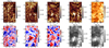 |
Fig. 5. Maps of the Hα line parameters. The spatial averages have been subtracted in the Doppler velocity maps. |
The maps of the source function provide information on temperature or radiation field at the different atmospheric levels. The map of Sp is very similar to the near-continuum intensity image at 0.4 nm off the line (see Fig. 2) and corresponds to the spatial distribution of the temperature at the continuum-forming level of the photosphere. The map of S0 is practically a reproduction of the core intensity image of the line (Fig. 2). This is expected because it is well known that the core of a very strong line is formed at the outer part of the atmosphere, and its intensity is expected to be very close to the source function at the formation level. The maps of S2 and S1 show the structure of the source function at the top level of the photosphere and at the lower level of the chromosphere, respectively. The map of S2 displays the inverse convective pattern consisting of dark cells and bright lanes, and the map of S1 is similar to that of S0.
Our spectral inversion produces the Doppler velocity maps at the three atmospheric levels (Fig. 5). These are very useful probes of the atmospheric dynamics. The map of vp shows the velocity pattern associated with granulation and photospheric oscillations, while the maps of v2 and v1 mostly show the velocity pattern linked to jet-like features and chromospheric oscillations. The similarity of v2 and v1 (with the Pearson correlation of 0.56) suggests that the difference in the oscillation phase between the lower chromosphere and the upper chromosphere is not large, implying that the wavelength of the associated waves may be longer than the height difference between the two layers.
The maps of either w2 or w1 of the Hα line (Fig. 5) provide a convenient way of distinguishing between the network regions and the internetwork regions. The network regions have high values of Doppler width and the internetwork regions have low values. The map of w1 practically corresponds to the temperature map in the upper atmosphere because the hydrogen atom is light and its thermal speed dominates the Doppler broadening.
Figure 6 shows the maps of the Ca II model parameters. Because the maps of Sp, S2, and S0 are very regular, they contain information on the spatial distribution of the physical parameters at the corresponding atmospheric level. The map of S0 is very similar to the core intensity image (Fig. 2). It is similar to the map of the Hαw1 in Fig. 5. On the other hand, the map of S1 is not regular in that it contains a number of discontinuities at different spatial scales.
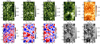 |
Fig. 6. Maps of the Ca II line parameters. The spatial averages have been subtracted in the Doppler velocity maps. |
The maps of vp, v2, and v1 of the Ca II band look very similar to those of the Hα line. It is expected that the Ca II band vp and the Hα band vp have very similar patterns (with the Pearson correlation of 0.88) because they were derived from two weak lines that formed in the photosphere. The similarities of the Ca IIv2 and the Hαv2 (correlation = 0.72) and that of the Ca IIv1 and the Hαv1 (correlation = 0.76) are more interesting. This supports the notion that the formation layer of the Ca II 854.2 nm line significantly overlaps that of the Hα line.
The maps of the Ca IIw2 and w1 are more complicated than those of the Hαw2 and w1. There is a tendency for w2 and w1 to be larger in the NW regions than in the IN regions. This tendency, however, is not as strong as in the Hα line. We find that numerous small patches of enhanced value of w1 are found to be scattered in the IN regions as well as in the NW regions.
We can estimate the random fitting errors by assuming that the physical conditions and systematic errors vary very smoothly with position so that their second-order spatial derivatives are approximately zero. Then we assume that the nonzero second-order finite difference of three neighboring points is contributed by the random errors. We applied this second-order derivative method to the variation in parameters along the slit direction at each slit position, which provides the estimates of the random error in each parameter. By repeating this process at a number of slit positions and by taking the average, we obtained the representative random errors of the mode parameters as listed in Table 3.
Representative random errors of the model parameters.
4.3. Inferring temperature and nonthermal speed
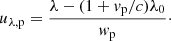
It is possible to separately determine the hydrogen temperature TH and the nonthermal speed (or microturbulence speed) ξ of the upper chromosphere by combining the values of w1 of the two lines. By denoting w1 of the Hα line by wH and that of the Ca II line by wCa, we can derive the expressions
![Mathematical equation: $$ \begin{aligned}&T_{\rm H} = 8100\,\mathrm{K}\,\left[ \frac{w_{\rm H}}{\mathrm{0.025\,nm}} \right]^2 \left( 1 - 0.59 \left[ \frac{w_{\rm Ca}}{w_{\rm H}}\right]^2 \right) \end{aligned} $$](/articles/aa/full_html/2020/08/aa38141-20/aa38141-20-eq24.gif) (23)
(23)
![Mathematical equation: $$ \begin{aligned}&\xi = 5.40\,\mathrm{km}\,\mathrm{s}^{-1}\,\frac{w_{\rm Ca}}{\mathrm{0.015\,nm}} \left( 1 - 0.042 \left[ \frac{w_{\rm H}}{w_{\rm Ca}}\right]^2 \right)^{1/2}, \end{aligned} $$](/articles/aa/full_html/2020/08/aa38141-20/aa38141-20-eq25.gif) (24)
(24)
which indicate that TH is mostly determined by wH because of the light mass of the hydrogen atom and ξ, mostly by wCa because of the high mass of a Ca II ion.
In the IN feature of Fig. 3, we have wH = 0.025 nm and wCa = 0.015 nm, which leads to the estimates T = 6500 K and ξ = 5.1 km s−1. In the NW feature of Fig. 4, we have wH = 0.036 nm and wCa = 0.023 nm in the Ca II line, which leads to the estimates T = 130 00 K and ξ = 7.8 km s−1.
Figure 7 shows the spatial distribution of TH and ξ determined from the Hα line w1 in Fig. 5 and the Ca II line w1 in Fig. 6. The map of TH is clearly very similar to the Hα line w1, and that of ξ, to the Ca II line w1. Making use of the second derivative method described above, we estimated the errors of TH and ξ at 140 K and 0.1 km s−1.
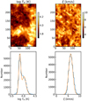 |
Fig. 7. Top: spatial distributions of TH and ξ. Bottom: number distributions of TH and ξ. |
The number distribution of TH is approximately a double Gaussian. The peak around 7000 K represents the typical temperature of the upper chromosphere in the IN regions and the other peak at 11 000 K, that in the NW regions. In contrast, the number distribution of ξ is singly peaked at 6.1 km s−1, which represents the typical ξ of the upper chromosphere, regardless of the specific region.
We confirm from Fig. 8 that S0 of the Ca II line is strongly correlated with TH. The Pearson correlation coefficient is 0.75. This means that the value of S0, or equivalently, the core intensity, is sensitive to temperature. This result supports the study of Cauzzi et al. (2009). The temperature sensitivity of the core intensity of Ca II line originates from the property of the Ca II line. In this line, the collisional excitation by electrons significantly contributes to the Ca II line emission. In contrast, the Hα line S0 or the core intensity is not correlated with TH at all, in agreement with Leenaarts et al. (2012), which means that the collisional excitation by electrons is less important in the Hα line emission. The Hα core intensity is correlated with the average formation height, with the lower intensity corresponding to the higher average formation height (Leenaarts et al. 2012).
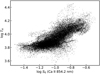 |
Fig. 8. Scatter plot of TH vs. the Ca II line S0. |
4.4. Temporal variations
It is interesting to determine the variation in model parameters with time at a fixed point. Figure 9 presents the line profiles of each line that were taken from an IN point and stacked over time (approximately one hour). The time epoch was set to the instant of the highest downflow speed. We find from the figure that the observed data (λ − t intensity maps) are fairly well reproduced by the corresponding models. The mean value of the fitting error ϵ was estimated at 0.0062 in the Hα line and at 0.014 in the Ca II line. The residual intensity maps show some systematic patterns that are correlated with the intensity distribution. Systematic errors seem to contribute significantly to the fitting errors. Some vertical patterns represent telluric lines and weak photospheric lines. These patterns are outside the clean wavelengths and were excluded in the inversion.
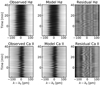 |
Fig. 9. Wavelength-time maps of the Hα and Ca II intensity stacked over time – observation (left) and model (middle), and maps of residual intensity normalized by the continuum intensity (right). The grey scale of the normalized residual intensity spans from −0.03 to 0.03. |
Figure 10 clearly indicates that all the model parameters as well as TH and ξ fluctuate with time. The standard deviations of the fluctuations are 2.4 km s−1 in the Hα line v1, 2.0 km s−1 in the Ca II line v1, 1100 K in TH, and 0.9 km s−1 in ξ. These are far larger than the estimates of the random errors 0.06 km s−1, 0.04 km s−1, 140 K, and 0.1 km s−1, respectively. Thus the fluctuations shown in Fig. 10 may represent the real variations in the physical conditions. The variations of v1 of the two lines represent chromospheric three-minute oscillations. The temporal variations of TH and ξ may be mostly attributed to the three-minute oscillations as well. The proper interpretation of the variations of TH and ξ in terms of chromospheric oscillations, however, is not straightforward, and requires further investigation to understand how the three-minute oscillations affect the formation of the two lines and their model parameters of the multiline spectral inversion. The three-minute oscillations in the upper chromosphere are now understood as highly nonlinear waves of very long wavelength that have sharp discontinuities, for example, shock fronts (Chae & Litvinenko 2017; Chae et al. 2018).
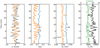 |
Fig. 10. Temporal variations of some of the model parameters as well as TH and ξ. |
5. Discussion
We proposed a multilayer spectral inversion in order to infer the physical condition of chromospheric plasma from strong absorption lines, and we specifically investigated the three-layer model in detail. This model is fully specified by 13 parameters. By fixing some parameters and determining one parameter from a weak line that is formed in the photosphere, we reduced the number of free parameters to 8 and determined these free parameters by applying the constrained nonlinear least-squares fitting. We found that the three-layer model reproduces most of the observed profiles of the Hα line and the Ca II 854.2 nm line taken from a quiet-Sun region fairly well. The random fitting errors are much smaller than the intrinsic spatial variations, therefore the maps of most model parameters look very regular. Thus, we conclude that our implementation of the spectral inversion is successful in determining the model parameters, and we have reached the first goal of successfully implementing the three-layer spectral inversion.
The ultimate goal of our investigation is to infer the physical conditions from the determined model parameters. This goal is distinct from the first goal and requires further investigation. The physical condition at each time is to be specified by the height variations in temperature, electron density, velocity, and nonthermal speed, but the determined model parameters are only a limited number of height-averaged source function, Doppler width, and line-of-sight velocity in each layer. Moreover, the spectral inversion does not provide any information on the height range of each layer. Hence, adopting some assumptions is indispensable to derive the physical conditions from the model parameters. The physical plausibility of the derived physical condition depends on the validity of the adopted assumptions.
For instance, hydrogen temperature TH and nonthermal speed ξ of the upper chromosphere were derived from the model parameters: wH and wCa, the Doppler widths of the Hα and the Ca II 854.2 nm lines based on the assumption that the upper chromosphere seen through the Ca II line is the same as the upper chromosphere seen through the Hα line. Under this assumption, the same values of TH and ξ contribute to both wH and wCa. In fact, TH is mostly determined by wH because a hydrogen atom is lighter and has a higher thermal speed than any other atoms or ions, as was previously noted by Cauzzi et al. (2009) and Leenaarts et al. (2012).
We determined TH and ξ in all the pixels of the observed quiet-Sun region and found that the distribution of the hydrogen temperature peaks at around 7000 K in the intranetwork regions, and around 11 000 K in network regions. The mean value of nonthermal speed is found to be 6 km s−1 regardless of intranetwork regions and network regions. Our measurements may be compared with the estimates of Cauzzi et al. (2009). They determined TH and ξ in a quiet region from the core widths of the two lines. Each core width was defined very like an FWHM and was directly measured from the line profile without taking the effect of radiative transfer into account. After subtracting the “intrinsic contribution” from the line widths that probably represents the opacity contribution to the line width, they obtained TH ranging from 5000 K to 60 000 K, and ξ ranging from 1 km s−1 to 11 km s−1. These ranges include and are broader than the corresponding ranges we obtained. Cauzzi et al. (2009) also noted that the core width of the Hα line is larger in the network patches, supporting the notion that network regions are heated more strongly than intranetwork ones.
The assumption used for the derivation of TH and ξ is reasonable, but it also has certain limitations. When we determine the volume-averaged values of TH and ξ in the upper chromosphere, the assumption seems to be good enough, as described above. If we were to determine the values in a fine Hα structure such as a fibril, the assumption is not satisfactory. The Hα fibrils are often invisible in the Ca II 854.2 nm line, which means that these plasma structures are transparent in the Ca II line. This may partly explain the lack of regional dependence on ξ we found above. ξ is mostly determined by the Doppler width of the Ca II line, but fibrils are transparent in the Ca II line, whereas they are clearly visible in the Hα line. If fibrils have higher temperature and higher nonthermal speed than the low-lying layers where the Ca II line is formed, it is likely that ξ in network regions was underestimated, and TH was overestimated.
Making better use of the determined model parameters requires a good understanding of the line formation. In this regard, one can learn much from the forward modelling of the non-LTE radiative transfer. The forward modelling is different from the spectral inversion in that it initially adopts the height variation of temperature, density, and velocity, and calculates the source function by solving the rate equations for level populations and can determine the formation height. The core intensity of a line is close to the source function in the outermost part of the line formation region. It is well known that the Hα source function in the outer layers is mostly determined by the radiation field and is not sensitive to local temperature, but sensitive to height (Leenaarts et al. 2012). In contrast, the Ca II line source function in the outer layers is still affected by the collisional excitation and is sensitive to the local electron temperature. This explains the strong correlation shown in Fig. 8 and the similarly strong correlation between the Hα core width and the Ca II 854.2 nm core intensity reported by Cauzzi et al. (2009).
Finally, we would like to mention that the effect of isotopic splitting may have to be investigated in the multilayer spectral inversion of the Ca II 854.2 line in the future. Leenaarts et al. (2014) investigated this effect on the bisector and inversions. They showed that the line core asymmetry and inverse C-shape of the bisector of the Ca II 854.2 nm line can be explained by the isotopic splitting: the larger difference in line-of-sight velocity difference of more than 2 km s−1 can result from this.
We conclude that the multilayer spectral inversion successfully infers the model parameters from the observed profiles of strong absorption lines. The model parameters can be used to derive the physical parameters of chromospheric plasma such as the temperature, when physically plausible assumptions are made and if the line formation is well understood. Determining subtle variations of physical parameters in space or in time requires further careful investigations. Combining the model parameters of several lines would be of much help in determining the height variation of physical parameters. We expect that the multiline multilayer spectral inversion will serve as a powerful tool to infer the physical parameters of chromospheric plasma from observations.
Acknowledgments
JC greatly appreciates Juhyung Kang’s assistance in the implementation of the method using the Python software. This research was supported by the National Research Foundation of the Korea (NRF-2019H1D3A2A01099143, NRF-2020R1A2C2004616), and by the Korea Astronomy and Space Science Institute under the R&D program(Project No. 2020-1-850-07) supervised by the Ministry of Science and ICT.
References
- Beckers, J. M. 1964, PhD Thesis, Sacramento Peak Observatory, Air Force Cambridge Research Laboratories, Mass., USA [Google Scholar]
- Cauzzi, G., Reardon, K., Rutten, R. J., Tritschler, A., & Uitenbroek, H. 2009, A&A, 503, 577 [NASA ADS] [CrossRef] [EDP Sciences] [Google Scholar]
- Chae, J. 2014, ApJ, 780, 109 [NASA ADS] [CrossRef] [Google Scholar]
- Chae, J., & Litvinenko, Y. E. 2017, ApJ, 844, 129 [CrossRef] [Google Scholar]
- Chae, J., Park, H.-M., Ahn, K., et al. 2013, Sol. Phys., 288, 1 [Google Scholar]
- Chae, J., Cho, K., Song, D., & Litvinenko, Y. E. 2018, ApJ, 854, 127 [NASA ADS] [CrossRef] [Google Scholar]
- Gu, X.-M., Lin, J., Li, K.-J., & Dun, J.-P. 1996, Ap&SS, 240, 263 [NASA ADS] [CrossRef] [Google Scholar]
- Heinzel, P., Mein, N., & Mein, P. 1999, A&A, 346, 322 [NASA ADS] [Google Scholar]
- Leenaarts, J., Carlsson, M., & Rouppe van der Voort, L. 2012, ApJ, 749, 136 [NASA ADS] [CrossRef] [EDP Sciences] [Google Scholar]
- Leenaarts, J., de la Cruz Rodríguez, J., Kochukhov, O., & Carlsson, M. 2014, ApJ, 784, L17 [NASA ADS] [CrossRef] [Google Scholar]
- Mein, N., Mein, P., Heinzel, P., et al. 1996, A&A, 309, 275 [NASA ADS] [Google Scholar]
- Ruiz Cobo, B., & del Toro Iniesta, J. C. 1992, ApJ, 398, 375 [NASA ADS] [CrossRef] [Google Scholar]
- Ruiz Cobo, B., & del Toro Iniesta, J. C. 1994, A&A, 283, 129 [NASA ADS] [Google Scholar]
- Rutten, R. J. 2008, in Hα as a Chromospheric Diagnostic, eds. S. A. Matthews, J. M. Davis, & L. K. Harra, ASP Conf. Ser., 397, 54 [Google Scholar]
- Skumanich, A., & Lites, B. W. 1987, ApJ, 322, 473 [Google Scholar]
- Steinitz, R., Gebbie, K. B., & Bar, V. 1977, ApJ, 213, 269 [CrossRef] [Google Scholar]
- Tsiropoula, G., Madi, C., & Schmieder, B. 1999, Sol. Phys., 187, 11 [NASA ADS] [CrossRef] [Google Scholar]
- Tziotziou, K. 2007, in Chromospheric Cloud-Model Inversion Techniques, eds. P. Heinzel, I. Dorotovič, & R. J. Rutten, ASP Conf. Ser., 368, 217 [Google Scholar]
- Unno, W. 1956, PASJ, 8, 108 [NASA ADS] [Google Scholar]
All Tables
All Figures
|
Fig. 1. Three-layer model of radiative transfer that consists of two chromospheric layers and one photospheric layer. |
| In the text | |
|
Fig. 2. Monochromatic images of a quiet region constructed at ten selected wavelengths. The two symbols mark the position of a intranetwork feature (x) and a network feature (+) selected for the illustration of the observed line profiles and the model fitting. |
| In the text | |
|
Fig. 3. Three-layer model fitting of the line profiles taken from an intranetwork feature marked by the cross in Fig. 2. The reference profile is the average of all the profiles over the observed region. |
| In the text | |
|
Fig. 4. Three-layer model fitting of the line profiles taken from a network feature marked by a plus in Fig. 2. |
| In the text | |
|
Fig. 5. Maps of the Hα line parameters. The spatial averages have been subtracted in the Doppler velocity maps. |
| In the text | |
|
Fig. 6. Maps of the Ca II line parameters. The spatial averages have been subtracted in the Doppler velocity maps. |
| In the text | |
|
Fig. 7. Top: spatial distributions of TH and ξ. Bottom: number distributions of TH and ξ. |
| In the text | |
|
Fig. 8. Scatter plot of TH vs. the Ca II line S0. |
| In the text | |
|
Fig. 9. Wavelength-time maps of the Hα and Ca II intensity stacked over time – observation (left) and model (middle), and maps of residual intensity normalized by the continuum intensity (right). The grey scale of the normalized residual intensity spans from −0.03 to 0.03. |
| In the text | |
|
Fig. 10. Temporal variations of some of the model parameters as well as TH and ξ. |
| In the text | |
Current usage metrics show cumulative count of Article Views (full-text article views including HTML views, PDF and ePub downloads, according to the available data) and Abstracts Views on Vision4Press platform.
Data correspond to usage on the plateform after 2015. The current usage metrics is available 48-96 hours after online publication and is updated daily on week days.
Initial download of the metrics may take a while.