| Issue |
A&A
Volume 640, August 2020
|
|
|---|---|---|
| Article Number | A96 | |
| Number of page(s) | 19 | |
| Section | Stellar structure and evolution | |
| DOI | https://doi.org/10.1051/0004-6361/202037960 | |
| Published online | 20 August 2020 | |
An optical spectroscopic and polarimetric study of the microquasar binary system SS 433
1
Dipartimento di Fisica “Enrico Fermi”, Università di Pisa, Pisa, Italy
e-mail: This email address is being protected from spambots. You need JavaScript enabled to view it.
2
INFN- Sezione Pisa, Largo B. Pontecorvo 3, 56127 Pisa, Italy
3
Astrophysics Research Institute, Liverpool John Moores University, IC2, LSP, 146 Brownlow Hill, Liverpool L3 5RF, UK
4
Department of Physics and Astronomy, University of Turku, 20014 Turku, Finland
Received:
13
March
2020
Accepted:
26
May
2020
Abstract
Aims. Our aim is to study the mass transfer, accretion environment, and wind outflows in the SS 433 system, concentrating on the so-called stationary lines.
Methods. We used archival high-resolution (X-shooter) and low-resolution (EMMI) optical spectra, new optical multi-filter polarimetry, and low-resolution optical spectra (Liverpool Telescope), spanning an interval of a decade and a broad range of precessional and orbital phases, to derive the dynamical properties of the system.
Results. Using optical interstellar absorption lines and H I 21 cm profiles, we derive E(B − V) = 0.86 ± 0.10, with an upper limit of E(B − V) = 1.8 ± 0.1 based on optical Diffuse Interstellar Bands. We obtain revised values for the ultraviolet and U band polarizations and polarization angles (PA), based on a new calibrator star at nearly the same distance as SS 433 that corrects the published measurement and yields the same PA as the optical. The polarization wavelength dependence is consistent with optical-dominating electron scattering with a Rayleigh component in U and the UV filters. No significant phase modulation was found for PA while there is significant variability in the polarization level. We fortuitously caught a flare event; no polarization changes were observed but we confirm the previously reported associated emission line variations. Studying profile modulation of multiple lines of H I, He I, O I, Na I, Si II, Ca II, Fe II with precessional and orbital phase, we derive properties for the accretion disk and present evidence for a strong disk wind, extending published results. Using transition-dependent systemic velocities, we probe the velocity gradient of the wind, and demonstrate that it is also variable on timescales unrelated to the orbit. Using the rotational velocity, around 140 ± 20 km s−1, a redetermined mass ratio q = 0.37 ± 0.04, and masses MX = 4.2 ± 0.4 M⊙, MA = 11.3 ± 0.6 M⊙, the radius of the A star fills – or slightly overfills – its Roche surface. We devote particular attention to the O I 7772 Å and 8446 Å lines, finding that they show different but related orbital and precessional modulation and there is no evidence for a circumbinary component. The spectral line profile variability can, in general, be understood with an ionization stratified outflow predicted by thermal wind modeling, modulated by different lines of sight through the disk produced by its precession. The wind can also account for an extended equatorial structure detected at long wavelength.
Key words: accretion, accretion disks / techniques: polarimetric / techniques: spectroscopic / binaries: close
© ESO 2020
1. Introduction
As the prototype Galactic microquasar, the binary system SS 433 (=V1343 Aql) has been extensively studied from TeV through low frequency radio and spatial resolutions down to the mas scale since its discovery. Much of this work has concentrated on its iconic jets and their phenomenology, the standard kinematic model for which is the precession of a tilted accretion disk around a compact, relativistic object (see Fabrika 2004, for a review) with a period of about 162 days. The jets move ballistically at about 0.26c into the surrounding supernova remnant W50. Their geometry and kinematics have been measured over decades since the first interferometric imaging in the 1980s (Hjellming & Johnston 1981). The inferred accretion rates are super-Eddington (see Fuchs et al. 2006; Shkovskii 1981; Kotani et al. 1996; Fabrika 1997) so the disk is likely thick and losing mass, with the supply of material coming from the companion that is presumed to fill (or overfill) its Roche surface (Hillwig et al. 2004). Efforts to unravel the nature of the gainer have concentrated on obtaining its mass, based mainly on emission line studies (Fabrika & Bychkova 1990; Fabrika 1997). The system is photometrically variable due to the partial eclipse of the gainer by the companion on a 13 day orbit. The photospheric lines of the loser (Hillwig et al. 2004) have been detected and it is identified as an early A supergiant. Combining the mass function, mass ratio, and eclipse solution, the range of masses for the gainer is consistent with a stellar mass black hole. The greatest attention has been paid, to date, on the inner portion of the accretion disk from which the jets emerge and that provide insights into processes under strong gravity that mimic active galactic nuclei. In this paper, in contrast, we focus on the accretion disk and its associated wind. Our aim is to present a unified description of the hydrodynamic processes inferred from low and high resolution optical spectroscopy and filter polarimetry.
2. Observations
The dataset used in this work combines new and archival material. The full journal of observations is presented in Appendix A. The new observations are multi-filter polarimetry and low-resolution spectroscopy, taken at the Liverpool Telescope (LT, La Palma, Spain) and the T60 telescope (Haleakala, Hawaii, USA), both operated remotely. Polarimetry data were obtained with the RINGO3 (LT) and Dipol-2 polarimeters (T60). The instruments simultaneously measure linear polarization in the B, V, and R bands (Arnold et al. 2012; Piirola et al. 2014). Dipol-2 data calibration was performed by the telescope personnel (see Kosenkov et al. 2017; Piirola et al. 2020). The spectroscopic dataset comprises new low-resolution data (see Barnsley et al. 2012), acquired at the LT with the FRODOSpec spectrograph, and archival low- and high-resolution ESO spectra, obtained from NTT and VLT telescopes, with EMMI and X-shooter spectrographs respectively1, see Table 1. Only the X-shooter spectra are flux-calibrated. The quantitative analysis presented here is based primarily on the EMMI and X-shooter spectra. The LT spectra were used for the study of an outburst detected during the observing campaign (see Sect. 5.2.7).
Observation modes specifics of the spectrographs: the wavelength coverage, the resolving power R and the total number N of the spectra per each instrument.
3. Data analysis: ISM extinction
3.1. ISM polarization contribution
The interstellar medium (ISM) component of the measured polarization was removed using comparison stars located in the same field of view of SS 433, as near as possible to the source in angle and distance from the Gaia DR2 data. This permitted the derivation of the Serkowski curve in that region of the sky and the determination of the ISM Stokes parameters. The stars for which the polarization was measured are S2, S5, following the notation of Leibowitz & Mendelson (1982), a new calibrator, SCal2. S2 and S5 were measured with Dipol-2 while SCal, because of its magnitude, required Dipol-UF3, a new polarimeter installed at the Nordic Optical Telescope (NOT), that is better suited for faint objects. The polarization measurements of these stars are listed in Table 2.
Polarization and magnitude (Gaia BP filter) parameters of the field stars S2, S5 and SCal.
The data in the three filters were fit with the Serkowski law (Serkowski et al. 1973). The measures for S2 and S5 are nearly the same in both the polarization level (PL) and the polarization angle (PA) (see Table 2), suggesting that the stars are intrinsically unpolarized and their polarization is probably only interstellar in origin. SCal, instead, indicates how the ISM induced polarization varies as the distance increases. This source is the physically nearest to SS 433. The fit parameters are listed in Table 3, together with the parallaxes measured by Gaia, which indicate that the stars are respectively located at about 1.1, 0.7 and 4 kpc from the Earth. SS 433 has a parallax of pSS433 = 0.22 ± 0.06, which corresponds to a distance of about 4.5 kpc. Using only S2 and S5 and interpolating the Serkowski pmax up to the SS 433 parallax, gives  , which is significantly lower than the value given by SCal. Moreover, the PA changes drastically. Thus, removing the interstellar contribution requires measuring the polarization of calibrators located spatially as near as possible to the source. For these reasons, SCal was used to obtain the intrinsic polarization values of SS 433. The interstellar Stokes parameters of the respective filters are provided in Table 4. The final Stokes parameters in the B, V, R filters were obtained using SCal while those in the U filter were obtained from the Serkowski law fit assuming the same PA of the B filter.
Parallaxes and Serkowski curves fitted.
SCal ISM Stokes parameters in the various filters.
3.2. ISM AV and E(B − V) determination
The total extinction coefficient, AV, was first derived by Wagner (1986) by fitting blackbody curves to optical spectrophotometric observations. He obtained AV = 7.8 ± 0.5 mag. We derived a range for E(B − V) and a value for AV, from two independent methods: (1) H I column density along the SS 433 line of sight and (2) the equivalent width (EW) of DIBs present in the spectra. Both are based on measurements of tracers that are external to SS 433 and do not require any assumptions regarding the system’s spectrum.
Güver & Özel (2009) obtained a calibration between the H I column density and the extinction,

The neutral hydrogen column density toward SS 433 is known from Galactic 21 cm profiles in the Leiden/Dwingeloo Survey for the sky north of −30° (Kalberla et al. 2005). We integrated the H I 21 cm profile over the interstellar Na I D1 velocity range and divided it by the integral of the entire H I 21 line to obtain the fraction of the total column density of H I toward that particular line of sight NH, tot = (6.40 ± 0.28)×1021 cm−2. For SS 433, we obtained NH, SS = (5.95 ± 0.29) × 1021 cm−2, AV = 2.69 ± 0.17 mag and E(B − V) = 0.86 ± 0.10 mag using a total to selective extinction ratio of 3.1. This estimate is much lower than Wagner (1986), but agrees with the value obtained by Margon et al. (1979), AV ∼ 2.3.
The DIBs are interstellar absorption transitions of still uncertain origin. Because of their ubiquity as a feature of the ISM, it is possible to derive E(B − V) from their EW, which is correlated to the reddening (Friedman et al. 2011; Lan et al. 2015). X-shooter spectra are used since they have the best signal to noise and resolution. We used the 5780 Å and 6614 Å bands. Two correlation laws have been used in this work: one, from Lan et al. (2015), relates the EW to E(B − V) through:

where A and γ are tabulated parameters that depend on the particular DIB considered. The other relation, from Friedman et al. (2011), is linear (see Table 4 of that paper for the correlation coefficients) and also depends on each DIB. We calculated the EWs for each of the 22 X-shooter spectra. The final values, shown in Table 5, were obtained taking the mean, weighted with the inverse of the variances. Given a DIB, the algorithm selects two continuum regions, one blueshifted and the other redshifted respect to the line, closely adjacent to it. It then calculates the EW, choosing a point in the blueward and another in the redward intervals. Repeating the procedure for all the combinations of the points in the given intervals yields a distribution of EWs, from which mean and standard deviation are obtained. The width of the continuum intervals (varied within a few Ås for each night) did not affect the mean EW, which remained consistent within the uncertainties. Table 5 also lists the H I column density using Friedman et al. (2011) since they found a better correlation with the H I column density (Fig. 2 of their paper) than E(B − V) (Fig. 4). Although near the limit of the reliable range of the correlations, the measured EWs give an indication of the upper limit to both the column density and extinction.
Reddening coefficients obtained from DIBs 5780 Å and 6614 Å.
Gies et al. (2002b) presented upper limits to the FUV (1150−1700 Å) flux of SS 433 using the Hubble Space Telescope (HST) applying the extinction from Wagner (1986) and Dolan et al. (1997) (who measured the SS 433 flux at 2770 Å with the High Speed Photometer (HSP) aboard HST) to extrapolate to the FUV. These UV observations further demonstrate that SS 433 is heavily reddened and that the AV and E(B − V) values we obtained are consistent and model-independent.
4. Data analysis: Spectroscopic variations
The spectroscopic data used in this work were sufficient to distinguish intrinsic and modulated changes in precessional and orbital phases (for details about the data, see Appendix A). The EMMI spectra covered a single, continuous sequence of observations. The system shows complex line profiles, which vary across transitions and in time (even from night to night), and modulated by the precession and orbital phases. Our analysis concentrates on the comparison of an ensemble of transitions from different species and arising from different processes to disentangle the line forming regions and dynamical environments.
Spectroscopically, although SS 433 has been studied mainly for the jet lines, the so called “stationary lines” that come from the binary system and trace the inner regions of the object and the accretion processes, leave many open questions. Usually, only a restricted set of lines have been studied, such as Hα, He II 4685 Å or the absorption features from the A-type supergiant (Crampton et al. 1980; Fabrika & Bychkova 1990; Blundell et al. 2008; Hillwig et al. 2004; Barnes et al. 2006), but SS 433 shows a wide variety of other transitions in the optical that can shed light on the binary environment. Some of these lines have already been reported, such as O I 8446, 7774 Å, the He I triplets (7065, 5875 Å) and singlets (6678 Å), and the Paschen lines, but their origin has been considered uncertain. It is not clear if they trace a region near the disk or if they come from more diffuse, circumstellar material. Most profiles for all species show both emission and absorption components, depending on the precessional phase, see Sect. 4.1. For this reason, the spectra have been studied as a function of both precessional and orbital phases. The ephemerides used in this work are from Goranskij (2011):


These are photometric and set the time of maximum brightness during the precession and the time of center of eclipse, respectively. The orbital phase ϕ = 0 is defined by the eclipse of the disk by the supergiant.
4.1. Precessional modulation
The precession alters the disk orientation to the line of sight. At phase ψ = 0 the disk is maximally face-on at 57° to the line of sight (Fabrika 2004)4. It is edge-on at phases ψ ∼ 0.3 and ψ ∼ 0.6. The lines that show absorption when the disk is edge-on all show the same modulation, so we concentrate on only one of them, He I 7065 Å, since it is the strongest. The Balmer sequence is not displayed since it is present only in the X-shooter spectra, for which the precessional and orbital phase coverage are not sufficient, see Appendix A. Hα is not shown because the EMMI data set is affected by an outburst (Blundell et al. 2011). Figure 1 shows the He I 7065 Å profile variations with the precessional phase at fixed orbital phase (near the first elongation, between 0.20 and 0.35). The letters in each plot title indicate the spectrograph: “X” for X-shooter, “E” for EMMI (best phase coverage) and “L” for Liverpool. The choice of the orbital phase does not affect the variations introduced by the disk precession.
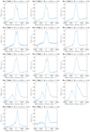 |
Fig. 1. He I 7065 Å line precessional sequence near the first elongation. The letters in each plot title indicate the spectrograph: “X” for X-shooter, “E” for EMMI (best phase coverage) and “L” for Liverpool. |
The absorption appears around ψ = 0.32 and persists to ψ = 0.48 (last spectrum), so the medium that produces the absorption is in the plane of the disk and is quite extended. Moreover, it is asymmetric relative to the disk plane, since no absorption is detected at ψ = 0.2 but it also persists during the second half of the disk precession, as it is shown by the X-shooter spectra (see Sect. 5.2.6). The red wing extends to +500 km s−1. The emission profile is asymmetric toward the red, especially when the disk is face-on and during primary eclipse; this is displayed by all the lines studied and is displayed in Fig. 2. The absorption appears when the disk is edge-on and is always blue-shifted (Fig. 1). This change in the profiles is long-term and systematic since it is present in both the EMMI and X-shooter spectra, although these were obtained more than ten years apart.
 |
Fig. 2. He I 7065 Å line orbital sequence when the disk is face-on. The letters in each plot title indicate the spectrograph: “X” for X-shooter, “E” for EMMI (best phase coverage) and “L” for Liverpool. |
4.2. Orbital modulation
The orbital motion of the system produces variations in the line profiles that are less pronounced than those caused by precession. The orbital modulation is shown at nearly face-on phases (0.90 < ψ < 0.10) since the induced variations in the profiles are seen better and not affected by the disk absorption. The orbital modulation is more visible in the core of the profiles and in their two peak structure (since many lines show the double peak structure, the term “blueshifted peak” is replaced by V and “redshifted peak” by R). The He I 7065 Å line will again be the focus since it displays well the general characteristics shown by all the lines (i.e., V/R on the core and the blueshifted absorption when the disk is edge-on). When the disk is face-on, in Fig. 2, He I 7065 Å line shows only the V/R structure in the core. R is more shifted and prominent at primary eclipse, the double peak structure then emerges, with V maximum at ϕ ∼ 0.2−0.3; V/R is symmetric at secondary eclipse. Finally, V decreases while R brightens. Hα, O I 8446 Å and all the other lines studied also show this pattern.
There is an asymmetry in velocity between the maximal redshift and blueshift. At ϕ ∼ 0, R reaches ∼ + 250 km s−1, while at phase ∼0.3 V is at around −100 to −125 km s−1. The core of the lines traces a different region than the blueshifted absorption that appears only when the disk is edge-on (Fig. 1). In particular, one spectrum in Fig. 2, at precessional phase ψ = 0.91, shows enhanced absorption near its core and detached blueshifted absorption at around −400 km s−1. These multiple features are present in many other lines (such as Fe II 5169 Å and Paschen series) but not in He II 4685 Å. As we discuss in Sect. 5.2.6, these multiple absorptions give important information on the dynamical environment present in this system; they are visible at other intermediate phases, but only during the second half of the precession. The variations of the V/R structure of these profiles with orbital phase displays a strict correspondence with the He II line, which shows V more intense at ϕ ∼ 0.2 and R more intense at ϕ ∼ 0.
4.3. Intrinsic line variations.
The high resolution, high S/N X-shooter spectra permitted an investigation of the intrinsic line profile variations of the system, that is, those that are due to neither precession nor the orbit. We studied line profiles from different nights at precessional and orbital phases as close as possible. Figure 3 shows the comparison between three transition: He II 4685 Å, He I 5875 Å and O I 8446 Å.
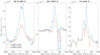 |
Fig. 3. Three different transitions at the same precessional and orbital phases. We note the clear differences in the profiles, and the blueshifted absorption features at negative velocities for He I 5875 Å. We note also the blueshifted absorption component of the Na I doublet in the He I 5875 Å subfigure. The lines have been plotted to the same continuum level for display. |
Although both phases are nearly identical (these are the only two spectra in the dataset that agree so closely in phase), there are clear differences in the line profiles. The He II 4686 Å profiles differ in the wings and peak ratios, He I 5875 Å at ϕ = 0.97 shows multiple, detached, weak absorption components while that at ϕ = 0.94 shows a single absorption at lower velocity. In addition, there is a peculiar absorption of the Na I doublet in both the spectra (see Fig. 4), detected for the first time in SS 433. The O I 8446 Å displays changes in the peak relative intensity and multiple weak features, while the FWZI of the profile remains the same. Figure 3 shows the transient changes in the flows present in the binary. All of these features can be detected only at high resolution, highlighting it as a crucial requirement for any future spectroscopic observations of SS 433. Without it, many features of the profiles will be undetectable and the analysis affected by systematics.
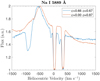 |
Fig. 4. Two X-shooter spectra showing Na I D1 at opposite precessional phases. The appearance of additional absorption components at ψ = 0.66 is important. The absorption was never detected at nearly face-on phases; it appears only when the disk is edge-on (also during the May sequence, ψ ∼ 0.86), indicating again that the disk is self-absorbing. |
5. Results
This section presents the picture of SS 433 that emerges from the data analysis, concentrating on the properties of the thick accretion disk and flows in the system.
5.1. Broadband filter polarimetry
The complete polarization data set is provided in Table B.6–B.8, which show the measured data, uncorrected for the ISM.
5.1.1. Photometric and polarimetric orbital variations.
The orbit-modulated ISM corrected polarimetric curves for SS 433 are shown in Figs. 5–7. The outburst night is plotted in black to distinguish it from the others. This event is not included in the discussion of the “normal” behavior of the system, but it will be considered in Sect. 5.2.7. All filters show a significant change of PL and PA only around primary eclipse, when the disk is occulted by the supergiant. The B filter shows a stronger modulation in PL and PA over the orbit with respect to the other filters. The most important change is observed during primary eclipse. All bands have higher PL at ϕ = 0, while the PA decrease is phase shifted by 0.1. To verify that the change of PL and PA over primary eclipse is significant, we compared the mean (weighted with the points dispersion) and standard deviation of the points near primary eclipse (specifically, between 0.9 ≤ ϕ ≤ 0.1) with the points located in the rest of the orbit, in all three filters. The significance level, SL = (PLE − PLOE)/σOE, has also been calculated for both PL and PA. The subscript “E” refers to the points near primary eclipse while “OE” signifies those outside that interval (i.e., outside eclipse). The results are listed in Table 6. The PL change during primary eclipse is more significant in the B and V filters and is higher in B (2.8σ). The PA presents the same significance level in all three filters (1.5−1.8σ). The PL variation around primary eclipse and the PA phase shift has not been reported previously since published studies have focused on the precession-related variation of the polarization, marginalized over the orbital modulation (Efimov et al. 1984; McLean & Tapia 1981). The phase dependent polarization variations are due to the compact object and its disk. One possibility is that although the disk is obscured, the scattering region is more extended and not as severely occulted. A contribution from the A star, by Rayleigh scattering around primary eclipse, could also be present. More detailed phase coverage with spectropolarimetric observations are needed to resolve this. The R filter displays the lowest orbital modulation: the filter probes cooler regions in the periphery of the accretion disk, and, perhaps, more extended structures. Our polarization sequence (Tables B.6–B.8), was obtained with the disk nearly edge-on. Were we observing a classical thin disk, the polarization would depend strongly on the angle between the line of sight and the disk orientation, and the PL and PA variations should be very pronounced as the disk tilts. This does not appear to be the case, and suggests that either the disk is not geometrically thin, or that the polarization is produced by an extended structure. Since the spectra show self absorption of the disk during the edge-on phase, the polarization should come from a more extended, optically thin region, which is dynamically tied to the gainer and the disk (because of the orbital modulation of PL and PA) but its structure is different. A higher PL at ϕ ∼ 0, in fact, can be due to dilution effects because of the eclipse of the disk or to the highlight of an extended coronal structure above the disk. The change in PL around primary eclipse is consistent with a continuum contribution from the disk coming with the scattered (polarizing) structure. Partial obscuration of the disk increases PL at primary eclipse. The relative contribution is consistent with what appears to be required for interpreting the secondary absorption line spectrum (see below and Sect. 5.2.2).
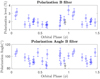 |
Fig. 5. Polarization light curve in the B filter. The outburst night is in black. |
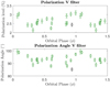 |
Fig. 6. Polarization light curve in the V filter. The outburst night is in black. |
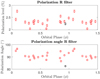 |
Fig. 7. Polarization light curve in the R filter. The outburst night is in black. |
Mean and standard deviations of PL and PA around primary eclipse and in the rest of the orbit.
5.1.2. Redetermination of the ultraviolet polarization and the presence of a Rayleigh scatterer
Because of its distance from the Earth and its location near the Galactic plane, polarimetric measurements for SS 433 were strongly affected by the ISM systematics. Efimov et al. (1984) assumed a wavelength independent intrinsic polarization in their five filters (UBVRI), and obtained a fit for the ISM Serkowski curve. They took the time dependence of their data to be the intrinsic variation and separated it from the constant ISM values. To derive the ISM PA, they considered the line connecting the R and I filter points in the Stokes parameters, assuming that the slope they derived coincided with the ISM PA. They obtained θ ∼ 3°, which is significantly different than the value we obtained.
Dolan et al. (1997) measured the polarization level of SS 433 in the UBVR filters from the ground, and in the ultraviolet at 2770 Å (UV) using the polarimetric filters on the High Speed Photometer (HSP) aboard the Hubble Space Telescope (HST). They chose S1 and S16 as references, for which they measured a PA ≈ 3.5° and PL ≈ 2%. After correction, they found a PA nearly parallel to the jet direction in the UV and V filter, while in the B, R and I filters it is ≈140°. Significantly, this difference between the B and V filters vanishes applying our correction (see Figs. 5–7). They also reported a marked increase in PL from the U to the UV, pU = 8.9 ± 0.9% and pUV = 18 ± 3%, and proposed that this can be due to Rayleigh scattering. Since Rayleigh and Thomson scattering have the same phase function, one would expect the same PA from the UV to the optical but, instead, they found PA ≈ 79° in the UV, ≈90° in U, and ≈140° in the visible. We obtain new intrinsic values for the U passband, applying our ISM correction: PLU = (10.28 ± 0.73)% and PAU = (90.9 ± 2.2)°. The new U and corrected V PAs show that the anomalies in Dolan et al. (1997) are due only to their decontamination procedure. The V filter shows the same PA as the others, and, most important, the new PA derived in the U filter is consistent with the PAs measured in the present work. It appears that the polarization has two contributions: Thomson scattering, which dominates in the optical; and Rayleigh scattering, which comes from the same scattering region as the optical bandpasses. The jets have a position angle in the sky of ∼100°, parallel to the PA in the U filter. Now, since the PL is always proportional to the optical depth τ in the optically thin limit, that is, PLλ ∼ τλ. If the polarization arises from an extended disk, the PA must be orthogonal to it if the scatterer is optically thin. The measured polarization is consistent with the disk and not the jets. As noted by Dolan et al. (1997), the ratio of the UV to optical polarization should be ≈16 from Rayleigh scattering alone. The lower observed ratio implies that both Rayleigh and Thomson scattering are contributing in this source. A further indication is that the ratio PLE/PLOE progressively decreases from the B to the R filter (see Figs. 5–7 and Table 6). This change can be due to a dilution effect of the disk, which emission is more weighted toward the UV part of the spectrum. Moreover, a less effective contribution of the eclipse in the other bands is also possible, that is, the emission in V and R comes from a more extended region.
5.2. Spectroscopic results
5.2.1. He II velocity curve
Since its discovery, many attempts had been made to derive masses for the components of SS 433, but there remains a considerable dispersion among the results. The derived mass of the compact star ranges from 1.4 M⊙ (Goranskij 2011) to 15 M⊙ (Bowler 2018). The orbital motion of the gainer is traced by the He II 4685 Å line. Fabrika & Bychkova (1990) were the first to derive a value for the mass function of the system. They obtained a semi-amplitude for the compact object of KX = 175 ± 20 km s−1 and a systemic velocity γ = −13 ± 13 km s−1 centered around precessional phase ψ ∼ 0, when the central part of the disk is presented nearly face-on. The He II line displays the double peak profile expected from a thin disk, but is highly variable and the relative peak intensities change with precessional phase. The consensus is that the He II 4685 Å has contributions besides the disk (for example, from an extended region that includes the base of the jets).
The determination of the velocity curve of the loser is far more difficult. Gies et al. (2002a,b) succeeded in distinguishing the spectrum of the companion. They identified a spectral region with many weak absorption lines of singly ionized metals, e.g., Fe II, that correspond to a A 4−7 supergiant spectrum. They took the supergiant HD 9233 as the reference star (the superposition of the choosen spectral region between SS 433 and HD 9233 is quite similar), and used cross correlation to obtain the radial velocities. This was subsequently refined by Hillwig et al. (2004) and Hillwig & Gies (2008). They determined MO = 12.3 ± 3.3 M⊙ for the A star and MX = 4.3 ± 0.8 M⊙ for the black hole (BH) (their radial velocity curve for the compact object is consistent with Fabrika & Bychkova 1990). They observed the system at ψ ∼ 0, to reduce the systematics arising from any disk flows, obtaining KO = 58.2 ± 3.1 km s−1 and γ = 73 ± 2 km s−1, where KO and γ are the semi-amplitude and systemic velocities, respectively. More recently, Kubota et al. (2010) used high resolution spectra confirming the results of Hillwig & Gies (2008), although they included the Hillwig & Gies (2008) data in their analysis. They derived the velocity curve of the compact object using four He II lines. They fix the systemic velocity obtained from the A star velocity curve, γO = (59.2 ± 2.5) km s−1.
We have refined the fit, adding the He II velocities from the X-shooter spectra at face-on presentation. The new velocity curve, assuming a circular orbit here and in all subsequent fits, is shown in Fig. 8. The velocities were measured by calculating the line center of flux following Kubota et al. (2010). The associated error depends on the line width and complexity; the line was not fitted by a profile function to avoid bias. The orbital parameters are shown in Table 7. The velocity semi-amplitude is consistent with Fabrika & Bychkova (1990). At ϕ ∼ 0.1−0.2 there are two points clearly separated from the curve that we did not include in the fit. We suggest that the line, even if mainly tracing the gainer’s orbital motion, has a variable contribution related to a stream-disk impact hot spot or a wind. During those nights no outburst was reported. We emphasize that this system can be strongly affected by transient line variations and other multiple components can modify the line profiles, although the overall profile is more stable.
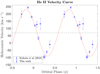 |
Fig. 8. Velocity curve of He II 4686 Å. The two points at ϕ ∼ 0.1−0.2 are probably affected by intrinsic variations in the line forming region and are not considered in the fit. |
Fit parameters of the binary components of SS 433.
5.2.2. Mass, radius and rotational velocity estimation of the A star
The Si II 6347 Å line showed weak absorption components at precessional phases 0.9 < ψ < 0.1 whose velocity changes with orbital phase. At these precessional phases, the lines are less affected by possible contamination from the disk. We exploit this new result in our final velocity curve without using cross correlations; the result is shown in Fig. 10 and the derived parameters are listed in Table 7. The values are consistent with those found by Kubota et al. (2010), Hillwig & Gies (2008). There is also agreement with the γ velocity of the He II curve, indicating, again, that these transitions trace the two components of SS 433, whose systemic velocity is higher than +60 km s−1. The A star lines are also detected at intermediate precessional phases. The Si II transitions are also present at near edge-on phases. They are partially blended with the disk Si II lines, but these are at higher velocity, stronger intensity in absorption, and narrower (see Fig. 9). No velocities were measured at these phases because of possible systematics affecting the lines. From the parameters in Table 7, we derived the masses of the SS 433 system: MO = 11.3 ± 0.6 M⊙ for the supergiant and MX = 4.2 ± 0.4 M⊙ for the compact object, indicating again that it is a low mass BH. For a circular orbit, Kepler’s third law yields the binary separation a = 0.271 ± 0.004 AU = 58.3 ± 0.9 R⊙. Using Eggleton (1983) for the Roche radius
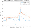 |
Fig. 9. Si II 6347 Å absorption at two different precessional phases. Only the A star absorption is present when the disk is face-on, while the disk also contributes at ψ ∼ 0.8. |
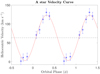 |
Fig. 10. Velocity curve of the A supergiant. The spectra chosen were when the disk was nearly face-on. See text for discussion. |
 (1)
(1)
where a and  are, respectively, the binary separation and the mass ratio of the two components, we obtain RL = 27.2 ± 2.6 R⊙. This is similar to Hillwig et al. (2004). We used the X-shooter spectra to estimate the radius (RO) and the equatorial rotational velocity Veq of the A star using the A4 Ib standard HD 59612 from the ESO archive, choosing the spectral region between 5200 Å and 5350 Å where the signal to noise of the X-shooter spectra was sufficiently high for the comparison, and selected the SS 433 spectrum at precessional phase ψ = 0.91, where the disk absorption line contribution is reduced. For simplicity we assume synchronism since tidal forces tend to enforce it on a timescale similar to that for circularization of the binary orbit (Zahn 1977; Frank et al. 2002). We note, however, that this is only an assumption in the absence of detailed evolutionary modeling of the progenitor system. We adopted a limb darkening parameter u = 0.5 for the convolving profile for a rigid rotator. Figure 11 shows the comparison of the SS 433 spectrum with the convolved profile of HD 59612. We also included a constant contaminating continuum from the disk, the level of which was adjusted during the comparison. The required value, about 50% of the flux at these wavelengths, is similar to that inferred from the PL variations during primary eclipse (Sect. 5.1.1). We used 80−160 km s−1, spanning the range in the literature, finding an acceptable match with Veq = (140 ± 20) km s−1. Assuming synchronous rigid body rotation gives a radius is RO = (36 ± 5) R⊙. This is somewhat higher than the Roche Lobe value we derived, consistent with the A star filling or overfilling its Roche lobe.
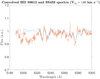 |
Fig. 11. Comparison between the A star standard spectrum diluted with a continuum contributing half the total light. |
5.2.3. Disk-wind and structure of the accretion disk
A blueshifted absorption, the signature of a net outflow, is seen when the disk is edge-on. This feature is persistent and varies similarly for all species on the precessional cycle. This has also been discussed by Fabrika (2004) and Fabrika et al. (1997), who tracked the velocity of the outflow as a function of precessional phase. When the disk is nearly face-on, vrad is high (from ∼ − 180 to ∼ − 1300 km s−1).
To search for orbital modulation of the absorption velocity, we chose the interval 0.2 ≤ ψ ≤ 0.4 where our phase coverage is good. The velocity curves were constructed from the EMMI spectra (we used only one X-shooter spectrum at the complementary phase ψ = 0.66) for all lines that show the absorption, that is, O I 7774 Å, O I 8446 Å, Pa 10−12, He I 7065 Å, He I 6678 Å and He I 5875 Å. We measured the velocity of the deep absorption, using the EMMI velocity resolution (25 km s−1) to estimate the uncertainty. All curves have been obtained near edge-on presentation of the disk except Fig. 14, at near face-on phases. These lines show clear orbital modulation with different amplitudes depending on the line formation regions. The curves are shown in Figs. 12–17. All of the radial velocity curves are synchronous in phase, apart from the O I 8446 Å, and vary with the same orbital period as He II 4686 Å. The Paschen velocities are shown together in Fig. 12 to manifest their close correspondence. Table 8 lists the fit parameters for each line. The aggregated Paschen line fit gives K = 130.3 ± 5.2 km s−1, ϕ = 0.43 ± 0.01 and γ = −139.1 ± 3.8 km s−1 with a χ2/ν = 3.88.
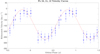 |
Fig. 12. Velocity curve of the three Paschen lines. The diamonds are the velocities of the Pa 12, the squares of Pa 11, and the stars of Pa 10. |
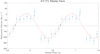 |
Fig. 13. Velocity curve of the O I 7774 Å line. |
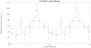 |
Fig. 14. Velocity curve of the O I 8446 Å line from the EMMI dataset when the disk is nearly edge-on. Some points were phase binned to improve the statistics since the resolution of the spectrographs is low (25 km s−1 px−1). This line is discussed in Sects. 5.2.3, 5.2.4 and 6. |
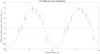 |
Fig. 15. Velocity curve of the O I 8446 Å line from X-shooter. The velocities are from the June dataset at nearly phase-on precessional phase and were cross correlated with the point at ϕ = 0.08. Superposing the γ velocity of the system (from the He II or Si II curve for example) gives a value in agreement with Fig. 14 and with the system velocity, indicating that this line does not come from the disk-wind. |
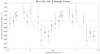 |
Fig. 16. Velocity curves of the He I Lines. The red line represents the global fit. The circles are the He I 7065 Å line while the black squares the He I 5875 Å. |
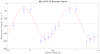 |
Fig. 17. Velocity curve of the He I 6678 Å. This curve has fewer points because some He I profiles were blended with the redshifted Hα jet line. |
Fit parameters of all the lines considered.
The Paschen lines, formed by recombination, show that the absorption when the disk is edge-on is due to self absorption by the disk and the wind. In contrast, the He I and O I velocity curves show different velocity amplitudes for lines of the same ion; different lines trace different regions.
The intercomparison of the velocity curves reveals a correlation of the systemic velocity, γ, with the velocity semi-amplitude, i.e., curves with similar velocity amplitudes show the same γ. Thus, the local environment sampled by each transition has a velocity component which is not purely orbital in the frame of the binary, or is coming from a different plane than the binary motion.
5.2.4. Wind velocity
The velocity curves indicate an outflow from the disk. From the precessional modulation of the absorption (Sect. 3) we infer that this structure is geometrically thick. The velocity of each transition at the optically thick surface, the Pseudo-photosphere (hereafter Pp), is given by Δγ, obtained from the difference between the individual velocity curves and the true systemic velocity from the He II curve. The velocities measured possess a component from the binary motion, and a component from the wind that is independent of orbital phase ϕ and depends only on the distance to the gainer. So, since every line traces a region whose distance from the gainer is fixed, Δγ should indicate the wind velocity at the line τ ≃ 1 surface for each transition. The wind velocities are shown in Fig. 18.
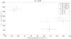 |
Fig. 18. Systemic velocities γj minus the system velocity (taken as that of He II) as function of the semi-amplitude velocities K. |
Figure 18 shows that He I 6678 Å singlet forms in a region where the wind gradient is higher, near the plane of the disk, and near the inner regions of the disk. In contrast, the He I triplet lines trace the outer part of the disk wind in height and radial distance. The O I 7774 Å and He I 6678 Å have similar intrinsic strengths (log gf) and trace the same part of the wind. The observed Paschen lines, from high members of the series, have similar velocities as He I 6678 Å; their optical depth is much lower than the principal Balmer lines.
Finally, Figs. 13–15 show that the O I 8446 Å and 7774 Å transitions sample different regions. The O I 7774 Å traces a structure that is circulating and outflowing, like the other transitions. The O I 8446 Å has a systemic velocity consistent with He II 4686 Å, while the 7774 Å multiplet shows the same shift as the Paschen lines. The O I absorption lines show that the disk and outflow self-absorb along the line of sight. The face-on systemic velocity is that of the BH indicating that the O I 7774 Å is optically thin for out-of-plane flow. Seen face-on, γ for O I 8446 Å again agrees with He II 4686 Å.
The phasing of the radial velocity for O I 7774 Å vs 8446 Å points to the latter arising mainly at the L1 point on the A star. Its presence as an emission line can be explained by Lyβ fluorescent excitation of the resonance transition at 1025 Å (e.g., Keenan & Hynek 1950), on exposure of the substellar point to the accretion disk (a Grotrian diagram is shown in Shore & Wahlgren 2010). This is the only line in the optical spectrum with these particular properties. The phase shift indicates multiple contributors with radial velocity variations, that is, the disk being in antiphase with the L1 point, but the relative amplitudes possibly changing over time. Another transition that forms because of radiative pumping is the Ca II 8662 Å Infrared Triplet (IRT). It is partially blended with Pa 13 and is very weak, but it is well distinguished in the X-shooter spectra taken between ψ = 0.86−0.89. Both transitions are shown Fig. 19. The IRT show two absorption components at ∼ − 150 and ∼ − 40 km s−1, while Pa 13 shows only the ∼ − 40 km s−1 feature. If the O I 8446 Å semi-amplitude is from orbital motion of L1, then it provides another estimate of the Roche radius, independent of the rotational velocity. Using the same argument as above, RRL ≈ 0.2a, which is consistent with that obtained from both the rotational analysis and the mass ratio for RRL. Thus, the combination of emission from material falling toward the gainer and being illuminated on the sub-stellar face of the loser appears to account for the observed O I 8446 Å variations. There is no need to invoke an orbiting circumsystem disk to account for the velocity and profile variations. Evidence based on profile decomposition as a set of independent contributors can also be affected in lower resolution spectra by intrinsic line profile variations that occur on timescales as short as a single period, such as the Hα variations reported by Blundell et al. (2008). Although a portion of the data set we used are the same spectra as Blundell et al. (2008), we reach a different conclusion when those are supplemented by higher resolution data. Further dynamical evidence for a circumbinary disk has been adduced from a similar decomposition analysis of the O I profile (e.g., Bowler 2010, 2011, 2013). The higher resolution data we have used in this study do not support this. Indeed, much of the variation in the relative peak intensities is due to variable absorption (e.g., Fig. 19) that have been treated as independent components in the published analyses.
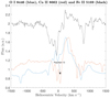 |
Fig. 19. O I 8446 Å, Ca II 8662 Å and Fe II 5169 Å transitions. The absorption features match in velocity. The Paschen 13 absorption feature is indicated by the arrow. The phase of the displayed spectrum is ψ = 0.87 and ϕ = 0.10. |
5.2.5. Estimate of the disk radius
An estimate of the disk radius is provided by the locale where the specific circular angular momentum is the same as that transferred through the L1 (Shu & Lubow 1981; Weiland et al. 1995). The specific angular momentum of the disk is  , where Mx is the mass of the gainer, and that carried by the stream is jstream = (1 − RRL/a)2a2Ω where Ω is the orbital frequency of the binary and a the separation of the components. Equating these gives rdisk/a = 0.30 for q = 0.37, that is, rdisk = 17 R⊙. In the end, 17 ≤ rdisk ≤ 31 R⊙, the upper limit coming from the binary separation and the A star Roche Lobe radius.
5.2.6. Multiple absorption components
An X-shooter spectrum from 2017 June 30.2 (ψ = 0.91, ϕ = 0.72), showed complex line profiles (the He I 7065 Å is shown in Fig. 1). The blueshifted absorption components at low and high velocity (e.g., He I 7065 Å, O I 7774 Å) suggest an intense mass ejection from the wind, revealed by mass loading of the outer parts of the outflow. Some lines, especially those from species with low ionization potentials (e.g., Fe+, C+, and Ca+) show the absorption only at high velocity, indicating that they are tracing the outer wind. If the picture outlined in Sect. 5.2.4 is correct then when the disk is nearly face-on, the full wind gradient is sampled by the line of sight. If the system undergoes an increased mass ejection, it may be possible to see the absorptions at low velocity even when the disk is face-on. We note that this event was not related to a flare of SS 433. That these properties are not unique is demonstrated by a second X-shooter sequence obtained on 2018 May 12.2−17.2 (0.86 ≤ ψ ≤ 0.89, 0.94 ≤ ϕ ≤ 0.25); see Fig. 19 as an example. Again, no flare was reported during this sequence. For Hβ, Hγ, and Hδ, the absorption extends to −450 km s−1 but the profile shows a sharp velocity maximum in the last spectrum. The redward emission wing extends to +800 km s−1 throughout the sequence. The emission component of the profile remains constant for the first four spectra but halves in the last spectrum. In the last spectrum of the 2018 sequence, the He I 5876 Å and 7065 Å lines also show enhanced absorption to −400 km s−1 and a persistent low velocity feature at −110 km s−1; in contrast, He I 6678 Å shows only the low velocity component. The Fe II lines 4921, 5018, and 5169 Å all show the same profiles as the He I triplets but with multiple components (−300, −200, −80 km s−1); only the lower two persist. The absorption profile is strongly phase dependent. Similar line profiles were also observed by Robinson et al. (2017) (see bottom panel of Fig. 2). The appearance of multiple, low dispersion absorptions points to an inhomogeneous and clumpy wind.
5.2.7. Spectra during the 2018 outburst
The LT sequence was fortuitously obtained during a radio outburst of SS 433, detected by Goranskij et al. (2018), it started on 2018 Jul 17.772 and ended on Jul 18.022 UT. At the same time, an increase in the optical brightness was detected up to R = 11.7, an increase of ∼2 mag above the mean value. The LT covered the last part of this burst. The photometry shows an increase in brightness for the orbital phase at which the burst started. Goranskij et al. (2018) reported increased emission only in He II 4686 Å. The LT spectrum, that covered only the red spectral interval, did not show any particular variation. The phase of the burst coincided with those of Kopylov et al. (1985) and Blundell et al. (2011). This coincidence between orbital phase and flaring activity may be pointing to an orbital ellipticity, as is known from other microquasars (e.g. LS+61° 303).
Polarimetric LT observations were also obtained for this night (black points from Figs. 5–7). No dramatic change was detected in either PL or PA during the burst night in any of the three filters.
The spectra show no particular changes until 23 days after the burst, corresponding to nearly two orbits, when three lines show far higher intensities and increased widths5. Figure 20 shows the comparison of Hα, He I 7065 Å and He I 6678 Å. The lines are very broad and display multiple features at high velocities, around ±1000 km s−1. In particular, Hα shows a double redshifted structure which persists for the whole observational interval. The neutral helium lines, instead, show the anomalous profile only on Aug 1.004 (ψ = 0.35, ϕ = 0.04). The subsequent spectra were taken six days later, so it is not possible to know the time scale over which they returned to quiescence. There are notable similarities in Fig. 20 between the three profiles during the burst, so the changes caused by the burst appear to be from a different region than that responsible for the quiescent lines.
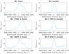 |
Fig. 20. Comparison of Hα, He I 7065 Å and He I 6678 Å before and during the burst. |
The common redshifted emission, +1000 km s−1 and the blue wing suggest that these lines, even if intrinsically different from each other and coming from different parts of the equatorial structure (see Sect. 5.2.3), show the same dynamical variation, perhaps the formation of outward propagating optically thin bright spots.
A comprehensive follow-up study of a radio burst of SS 433 was presented by Blundell et al. (2011) using the same EMMI spectroscopic data set of Blundell et al. (2008) that we used in this work. Beginning at a phase where the spectra were normal, Hα started to show the extended redshifted wings. They observed that after five days the jet lines intensified and their velocities (β ∼ 0.28−0.29) increased. Three days later, a type 1 radio flare occurred. The new LT spectra agree with the flaring line profile behavior described by Blundell et al. (2011). Goranskij et al. (2018) found enhanced He II line the same day of the burst. It is the only line that shows an instantaneous response to the flare, meaning that the flare comes from the inner parts of the accretion disk. The fact that Hα and, most important, the He I lines show a change in the profiles days after the burst is indicative of a delayed response of the accretion disk to the flare. From the velocity curves derived in this work, moreover, the line forming regions are known for He I 7065 Å and He I 6678 Å so it appears that the profile changes are from the disk-wind. The constancy of PL and PA, on the other hand, indicates that the outburst does not affect the scattering structure.
6. Conclusions
Concentrating on the spectral sequence from the near edge-on presentation of the disk permits a separation of the circulatory and outflow motions of the disk gas. The outflow, indicated by the P Cyg lines, appears tied to the orbital motion of the gainer. Choosing those transitions, that are sufficiently optically thick, here labelled j, that we can locate the Pp from the absorption edges, we measured their orbitally modulated radial velocity amplitude, Kj and systemic velocity, γj. We assume as symmetric outflow from the gainer as the basic geometry, whether axial or spherical is not important. Then the difference between γHe II and γj parameterizes the outflow at the Pp and the amplitude Kj gives the distance of that surface from the binary center of mass. We note that for all lines showing a strong P Cyg absorption component, γj < 0. Although non-axisymmetric structures complicate this picture, as do the stream and hot spot, this should not compromise the mapping of the velocity for the low ionization species we used. The outflow is ionization stratified. Since the central engine is the ionizing source, we would expect that those lines tracing progressively higher ionization states will have smaller velocity amplitudes. The O I transitions are especially important in tracing this because neutral oxygen is partially shielded by hydrogen; consequently, O I lines should be formed in the peripheral regions of the disk but within the region traced by the ionized metals. The Paschen lines are formed by recombination but those we have available are high in the series and weaker than the principal Balmer lines, so they probe deeper portions of the outflow. Further information is provided by the orbital modulation as a function of phase. When seen nearly face-on, the He I lines, for instance, do not show a P Cyg absorption trough and have greater widths but still vary in radial velocity. Together, this suggests a flaring wind of the sort modeled by Higginbottom et al. (2017) in which there is an acceleration and outflow from above the disk in a sort of biconical geometry. The weaker lines, especially Fe II and Si II, also probe deeper portions of the wind. The derived velocity gradient, shown in Fig. 18, is consistent with a slow acceleration of the outflow and will help constrain models of the line formation. We leave that for future work. We cannot derive a mass loss rate directly from these measurements without a better handle on the opening angle of the flow, but the dynamics are consistent with a slow, weakly collimated wind like those from the hydrodynamic simulations. A wind also accounts for the narrow absorption components. These are confined within the velocity range of the broader P Cyg absorption trough but vary sporadically over time. The integrated strengths of the disk lines vary, as well so these features may be like the discrete absorption features seen in hot star winds. With our limited coverage over the long term, however, we cannot determine whether a thermal wind or radiative acceleration is responsible for the driving.
For details about the EMMI dataset see Blundell et al. (2011) while the X-shooter data set corresponds to the ESO Program Id: 0101.D-0696 and P.I.: Waisberg, Idel (the dataset is published, in part, in Waisberg et al. 2019).
2MASS id source: 19114434+0459264.
For a description of the polarimeter, see http://www.not.iac.es/instruments/dipol-uf/DIPol-UF_description.html
Throughout the paper, the precessional phase is indicated with ψ and the orbital with ϕ.
The Hα line shows no intensity increase but it forms over a very spatially extended region and may be less sensitive to the more local changes induced in the disk following a burst. Unlike the He I lines, there were other nights for which Hα showed an enhanced peak to continuum ratio.
Acknowledgments
We thank Vilppu Piirola for the Dipol-2 and Dipol-UF observations. P.P. and S.N.S. thank Linda Schmidtobreick for generously furnishing the EMMI spectra and Anatol Cherepashchuk for correspondence. P.P. thanks Ferdinando Patat for crucial information on polarimetry data reduction and analysis given at the polarimetry school in Padova “Looking at Cosmic Sources in Polarized Light”. We acknowledge support from the ERC Advanced Grant HotMol ERC-2011-AdG-291659. The Dipol-2 and Dipol-UF polarimeters were built in cooperation by the University of Turku, Finland, and the Leibniz Institut für Sonnenphysik, Germany, with support from the Leibniz Association grant SAW-2011-KIS-7. We are grateful to the Institute for Astronomy, University of Hawaii, for the allocated observing time. Based on observations made with the Nordic Optical Telescope, operated by the Nordic Optical Telescope Scientific Association at the Observatorio del Roque de los Muchachos, La Palma, Spain, of the Instituto de Astrofisica de Canarias. Based on data obtained from the ESO Science Archive Facility. We thank the referee for insightful questions, particularly those focused on the polarization results.
References
- Arnold, D. M., Steele, I. A., Bates, S. D., Mottram, C. J., & Smith, R. J. 2012, in RINGO3: A Multi-colour Fast Response Polarimeter, SPIE Conf. Ser., 8446, 84462J [Google Scholar]
- Barnes, A. D., Casares, J., Charles, P. A., et al. 2006, MNRAS, 365, 296 [NASA ADS] [CrossRef] [Google Scholar]
- Barnsley, R. M., Smith, R. J., & Steele, I. A. 2012, Astron. Nachr., 333, 101 [NASA ADS] [CrossRef] [Google Scholar]
- Blundell, K. M., Bowler, M. G., & Schmidtobreick, L. 2008, ApJ, 678, L47 [Google Scholar]
- Blundell, K. M., Schmidtobreick, L., & Trushkin, S. 2011, MNRAS, 417, 2401 [NASA ADS] [CrossRef] [Google Scholar]
- Bowler, M. G. 2010, A&A, 521, A81 [NASA ADS] [CrossRef] [EDP Sciences] [Google Scholar]
- Bowler, M. G. 2011, A&A, 531, A107 [Google Scholar]
- Bowler, M. G. 2013, A&A, 556, A149 [NASA ADS] [CrossRef] [EDP Sciences] [Google Scholar]
- Bowler, M. G. 2018, A&A, 619, L4 [Google Scholar]
- Crampton, D., Cowley, A. P., & Hutchings, J. B. 1980, ApJ, 235, L131 [NASA ADS] [CrossRef] [Google Scholar]
- Dolan, J. F., Boyd, P. T., Fabrika, S., et al. 1997, A&A, 327, 648 [NASA ADS] [Google Scholar]
- Efimov, I. S., Shakhovskoi, N. M., & Piirola, V. 1984, A&A, 138, 62 [Google Scholar]
- Eggleton, P. P. 1983, ApJ, 268, 368 [NASA ADS] [CrossRef] [Google Scholar]
- Fabrika, S. 2004, Astrophys. Space Phys. Res., 12, 1 [Google Scholar]
- Fabrika, S. N. 1997, Ap&SS, 252, 439 [Google Scholar]
- Fabrika, S. N., & Bychkova, L. V. 1990, A&A, 240, L5 [NASA ADS] [Google Scholar]
- Fabrika, S. N., Bychkova, L. V., & Panferov, A. A. 1997, Bull. Spec. Astrophys. Obs., 43, 75 [Google Scholar]
- Frank, J., King, A., & Raine, D. J. 2002, Accretion Power in Astrophysics: Third Edition (Cambridge: Cambridge University Press) [Google Scholar]
- Friedman, S. D., York, D. G., McCall, B. J., et al. 2011, ApJ, 727, 33 [NASA ADS] [CrossRef] [Google Scholar]
- Fuchs, Y., Koch Miramond, L., & Ábrahám, P. 2006, A&A, 445, 1041 [NASA ADS] [CrossRef] [EDP Sciences] [Google Scholar]
- Gies, D. R., McSwain, M. V., Riddle, R. L., et al. 2002a, ApJ, 566, 1069 [NASA ADS] [CrossRef] [Google Scholar]
- Gies, D. R., Huang, W., & McSwain, M. V. 2002b, ApJ, 578, L67 [NASA ADS] [CrossRef] [Google Scholar]
- Goranskij, V. 2011, Peremennye Zvezdy, 31, 5 [NASA ADS] [Google Scholar]
- Goranskij, V. P., Barsukova, E. A., Burenkov, A. N., & Trushkin, S. A. 2018, ATel, 11870, 1 [Google Scholar]
- Güver, T., & Özel, F. 2009, MNRAS, 400, 2050 [NASA ADS] [CrossRef] [Google Scholar]
- Higginbottom, N., Proga, D., Knigge, C., & Long, K. S. 2017, ApJ, 836, 42 [Google Scholar]
- Hillwig, T. C., & Gies, D. R. 2008, ApJ, 676, L37 [NASA ADS] [CrossRef] [Google Scholar]
- Hillwig, T. C., Gies, D. R., Huang, W., et al. 2004, ApJ, 615, 422 [Google Scholar]
- Hjellming, R. M., & Johnston, K. J. 1981, Nature, 290, 100 [NASA ADS] [CrossRef] [EDP Sciences] [Google Scholar]
- Kalberla, P. M. W., Burton, W. B., Hartmann, D., et al. 2005, A&A, 440, 775 [NASA ADS] [CrossRef] [EDP Sciences] [Google Scholar]
- Keenan, P. C., & Hynek, J. A. 1950, ApJ, 111, 1 [NASA ADS] [CrossRef] [Google Scholar]
- Kopylov, I. M., Kumajdogodskaya, R. N., & Somova, T. A. 1985, AZh, 62, 323 [Google Scholar]
- Kosenkov, I. A., Berdyugin, A. V., Piirola, V., et al. 2017, MNRAS, 468, 4362 [NASA ADS] [CrossRef] [Google Scholar]
- Kotani, T., Kawai, N., Matsuoka, M., & Brinkmann, W. 1996, PASJ, 48, 619 [NASA ADS] [CrossRef] [Google Scholar]
- Kubota, K., Ueda, Y., Fabrika, S., et al. 2010, ApJ, 709, 1374 [NASA ADS] [CrossRef] [Google Scholar]
- Lan, T.-W., Ménard, B., & Zhu, G. 2015, MNRAS, 452, 3629 [Google Scholar]
- Leibowitz, E. M., & Mendelson, H. 1982, PASP, 94, 977 [NASA ADS] [CrossRef] [Google Scholar]
- Margon, B., Ford, H. C., Katz, J. I., et al. 1979, ApJ, 230, L41 [NASA ADS] [CrossRef] [Google Scholar]
- McLean, I. S., & Tapia, S. 1981, Vistas Astron., 25, 45 [CrossRef] [Google Scholar]
- Piirola, V., Berdyugin, A., & Berdyugina, S. 2014, in DIPOL-2: A Double Image High Precision Polarimeter, SPIE Conf. Ser., 9147, 91478I [Google Scholar]
- Piirola, V., Berdyugin, A., Frisch, P. C., et al. 2020, A&A, 635, A46 [CrossRef] [EDP Sciences] [Google Scholar]
- Robinson, E. L., Froning, C. S., Jaffe, D. T., et al. 2017, ApJ, 841, 79 [NASA ADS] [CrossRef] [Google Scholar]
- Serkowski, K. 1973, in Interstellar Dust and Related Topics, eds. J. M. Greenberg, & H. C. van de Hulst, IAU Symp., 52, 145 [CrossRef] [Google Scholar]
- Shkovskii, I. S. 1981, Sov. Astron., 25, 315 [Google Scholar]
- Shore, S. N., & Wahlgren, G. M. 2010, A&A, 515, A108 [NASA ADS] [CrossRef] [EDP Sciences] [Google Scholar]
- Shu, F. H., & Lubow, S. H. 1981, ARA&A, 19, 277 [NASA ADS] [CrossRef] [Google Scholar]
- Wagner, R. M. 1986, ApJ, 308, 152 [NASA ADS] [CrossRef] [Google Scholar]
- Waisberg, I., Dexter, J., Olivier-Petrucci, P., Dubus, G., & Perraut, K. 2019, A&A, 624, A127 [CrossRef] [EDP Sciences] [Google Scholar]
- Weiland, J. L., Shore, S. N., Beaver, E. A., Lyons, R. W., & Rosenblatt, E. I. 1995, ApJ, 447, 401 [NASA ADS] [CrossRef] [Google Scholar]
- Zahn, J. P. 1977, A&A, 57, 383 [Google Scholar]
Appendix A: Journal of observations
Tables A.1 and A.2 respectively show the journal of observations of X-shooter and FRODOSpec spectrographs. For the EMMI dataset, see Blundell et al. (2011), as mentioned in Sect. 2. The journal of polarization data is shown in Appendix B.
Journal of the spectra obtained from the X-shooter spectrograph.
Journal of spectroscopic observations from the Liverpool telescope; some nights overlap with the X-shooter observations.
Journal of polarimetric observations, Dipol-2.
Appendix B: Complementary data: Polarization and radial velocities of He II 4686 Å, Si II 6347 Å
The complete dataset of the polarization data and the radial velocities of the He II and Si II curves (Figs. 8 and 10) are shown in this section. Only the measured data are shown to avoid to weigh down the text. The second row of Tables B.6–B.8 contains the data from the burst night.
Measured radial velocities of the He II 4686 Å transition.
Measured radial velocities of the Si II 6347 Å transition.
Measured radial velocities of the Pa 10, 11, 12 transitions.
Measured radial velocities of the He I 7065, 5875, 6678 Å transitions.
Measured radial velocities of the O I 7774, 8446 Å transitions.
Measured polarization values in the B filter.
Same as Table B.6 for the V filter.
Same as Table B.6 for the R filter.
All Tables
Observation modes specifics of the spectrographs: the wavelength coverage, the resolving power R and the total number N of the spectra per each instrument.
Polarization and magnitude (Gaia BP filter) parameters of the field stars S2, S5 and SCal.
Mean and standard deviations of PL and PA around primary eclipse and in the rest of the orbit.
Journal of spectroscopic observations from the Liverpool telescope; some nights overlap with the X-shooter observations.
All Figures
|
Fig. 1. He I 7065 Å line precessional sequence near the first elongation. The letters in each plot title indicate the spectrograph: “X” for X-shooter, “E” for EMMI (best phase coverage) and “L” for Liverpool. |
| In the text | |
|
Fig. 2. He I 7065 Å line orbital sequence when the disk is face-on. The letters in each plot title indicate the spectrograph: “X” for X-shooter, “E” for EMMI (best phase coverage) and “L” for Liverpool. |
| In the text | |
|
Fig. 3. Three different transitions at the same precessional and orbital phases. We note the clear differences in the profiles, and the blueshifted absorption features at negative velocities for He I 5875 Å. We note also the blueshifted absorption component of the Na I doublet in the He I 5875 Å subfigure. The lines have been plotted to the same continuum level for display. |
| In the text | |
|
Fig. 4. Two X-shooter spectra showing Na I D1 at opposite precessional phases. The appearance of additional absorption components at ψ = 0.66 is important. The absorption was never detected at nearly face-on phases; it appears only when the disk is edge-on (also during the May sequence, ψ ∼ 0.86), indicating again that the disk is self-absorbing. |
| In the text | |
|
Fig. 5. Polarization light curve in the B filter. The outburst night is in black. |
| In the text | |
|
Fig. 6. Polarization light curve in the V filter. The outburst night is in black. |
| In the text | |
|
Fig. 7. Polarization light curve in the R filter. The outburst night is in black. |
| In the text | |
|
Fig. 8. Velocity curve of He II 4686 Å. The two points at ϕ ∼ 0.1−0.2 are probably affected by intrinsic variations in the line forming region and are not considered in the fit. |
| In the text | |
|
Fig. 9. Si II 6347 Å absorption at two different precessional phases. Only the A star absorption is present when the disk is face-on, while the disk also contributes at ψ ∼ 0.8. |
| In the text | |
|
Fig. 10. Velocity curve of the A supergiant. The spectra chosen were when the disk was nearly face-on. See text for discussion. |
| In the text | |
|
Fig. 11. Comparison between the A star standard spectrum diluted with a continuum contributing half the total light. |
| In the text | |
|
Fig. 12. Velocity curve of the three Paschen lines. The diamonds are the velocities of the Pa 12, the squares of Pa 11, and the stars of Pa 10. |
| In the text | |
|
Fig. 13. Velocity curve of the O I 7774 Å line. |
| In the text | |
|
Fig. 14. Velocity curve of the O I 8446 Å line from the EMMI dataset when the disk is nearly edge-on. Some points were phase binned to improve the statistics since the resolution of the spectrographs is low (25 km s−1 px−1). This line is discussed in Sects. 5.2.3, 5.2.4 and 6. |
| In the text | |
|
Fig. 15. Velocity curve of the O I 8446 Å line from X-shooter. The velocities are from the June dataset at nearly phase-on precessional phase and were cross correlated with the point at ϕ = 0.08. Superposing the γ velocity of the system (from the He II or Si II curve for example) gives a value in agreement with Fig. 14 and with the system velocity, indicating that this line does not come from the disk-wind. |
| In the text | |
|
Fig. 16. Velocity curves of the He I Lines. The red line represents the global fit. The circles are the He I 7065 Å line while the black squares the He I 5875 Å. |
| In the text | |
|
Fig. 17. Velocity curve of the He I 6678 Å. This curve has fewer points because some He I profiles were blended with the redshifted Hα jet line. |
| In the text | |
|
Fig. 18. Systemic velocities γj minus the system velocity (taken as that of He II) as function of the semi-amplitude velocities K. |
| In the text | |
|
Fig. 19. O I 8446 Å, Ca II 8662 Å and Fe II 5169 Å transitions. The absorption features match in velocity. The Paschen 13 absorption feature is indicated by the arrow. The phase of the displayed spectrum is ψ = 0.87 and ϕ = 0.10. |
| In the text | |
|
Fig. 20. Comparison of Hα, He I 7065 Å and He I 6678 Å before and during the burst. |
| In the text | |
Current usage metrics show cumulative count of Article Views (full-text article views including HTML views, PDF and ePub downloads, according to the available data) and Abstracts Views on Vision4Press platform.
Data correspond to usage on the plateform after 2015. The current usage metrics is available 48-96 hours after online publication and is updated daily on week days.
Initial download of the metrics may take a while.