| Issue |
A&A
Volume 640, August 2020
|
|
|---|---|---|
| Article Number | A34 | |
| Number of page(s) | 8 | |
| Section | Cosmology (including clusters of galaxies) | |
| DOI | https://doi.org/10.1051/0004-6361/202037584 | |
| Published online | 06 August 2020 | |
Evidence for radially independent size growth of early-type galaxies in clusters⋆
INAF–Osservatorio Astronomico di Brera, via Brera 28, 20121 Milano, Italy
e-mail: stefano.andreon@brera.inaf.it
Received:
27
January
2020
Accepted:
10
June
2020
It is not well understood whether the growth of early-type cluster galaxies proceeds inside-out, outside-in, or at the same pace at all radii. In this work we measured the galaxy size, defined by the radius including 80% of the galaxy light, non-parametrically. We also determined a non-parametric estimate of galaxy light concentration, which measures the curvature of the surface brightness profile in the galaxy outskirts. We used an almost random sampling of a mass-limited sample formed by 128 morphologically early-type galaxies in clusters with log M/M⊙ ≳ 10.7 spanning the wide range 0.17 < z < 1.81. From these data we derived the size-mass and concentration-mass relations, as well as their evolution. At 80% light radius, early-type galaxies in clusters are about 2.7 times larger than at 50% radius at all redshifts, and close to de Vaucouleurs profiles in the last 10 Gyr. While between z = 2 and z = 0 both half-light and 80% light sizes increase by a factor of 1.7, concentration stays constant within 2%, that is to say the size growth of early-type galaxies in cluster environments proceeds at the same pace at both radii. Existing physical explanations proposed in the literature are inconsistent with our results, demonstrating the need for dedicated numerical simulations to identify the physical mechanism affecting the galaxy structure.
Key words: Galaxy: evolution / galaxies: elliptical and lenticular, cD / galaxies: clusters: general
Full Table 1 is only available at the CDS via anonymous ftp to cdsarc.u-strasbg.fr (130.79.128.5) or via http://cdsarc.u-strasbg.fr/viz-bin/cat/J/A+A/640/A34
© ESO 2020
1. Introduction
Among massive galaxies, early-type galaxies (i.e., elliptical and lenticular) are the more abundant population in clusters up to z = 1.2 at least (Raichoor & Andreon 2012). Their size slowly grows with time and almost doubles beginning at z = 2 (at a fixed log M/M⊙ = 11 mass, Andreon et al. 2016; see also Strazzullo et al. 2010) at half the speed compared to identically selected galaxies in the field (Andreon 2018). It is not well understood if their size growth proceeds inside-out, outside-in, or at the same pace at all radii. By selecting galaxies on the red sequence, De Propris et al. (2016) find an evolution in the distribution of galaxy concentrations at z > 1 due to the appearance of galaxies with very low Sersic indices (n ∼ 1, i.e., highly concentrated). However, the sample they studied was not selected morphologically and indeed some of the high redshift concentrated galaxies are just clumpy systems (De Propris et al. 2016), which are rare in the local Universe. This emphasizes the importance of controlling for morphological composition in evolutionary studies. In the field environment, various works (e.g., van Dokkum et al. 2010; Patel et al. 2012) found lower Sersic indices at high redshift and interpret this as being due to a gradual build-up of the galaxy outer envelopes.
Major and minor dry mergers are expected to evolve galaxies in different ways in the mass-concentration plane (Hilz et al. 2013, see also Nipoti et al. 2003); dry minor mergers mostly alter concentration, while dry major mergers mostly change mass. In the IllustrisTNG simulation, galaxies with log M/M⊙ = 11 (for a Salpeter initial mass function (IMF)), which are mostly quiescent, have low concentrations because a large fraction of their mass comes from stars that formed in other galaxies and preferentially deposited in the galaxy outskirts (Tacchella et al. 2019). Less concentrated galaxies have larger fractions of stellar mass formed ex situ, that is to say in other galaxies (Tacchella et al. 2019). In other terms, the concentration is informative about the processes that shape the structure of early-type galaxies and is a direct tracer of where star formation initially occurred and the amount of mass acquired.
In this work we address the way by which galaxies grow in size by measuring the radial dependence of the size growth of early-type galaxies in clusters. We investigate the evolution of the concentration of a morphologically-selected, mass-limited sample of early-type galaxies in clusters.
Galaxies have no sharp boundaries. Traditionally, galaxy sizes are defined to include an arbitrary percentage of the total flux, almost always 50% (see Miller et al. 2019 for an exception). This choice is arbitrary and the inferred size evolution could be biased if galaxies change concentration while changing size. It is therefore important to extend the study of the mass-size relation to other radius definitions and explore the possible influence of a concentration evolution. In this work we adopt an 80% light size and we investigate the mass-size relation and its evolution with these sizes.
Two term clarifications are in order: first, size, compactness, and concentration are different concepts; second, different studies have different definitions of low and high concentrations. Compactness refers to the size of a galaxy at a fixed mass. When a galaxy is much smaller than the average for its mass, it is called compact (or over-dense). Compactness is a measure of difference in the surface brightness slope compared to the average for the same mass. Compactness and concentration are not synonyms; concentration is a measure of the profile curvature. Large Sersic index n are profiles for which the ratio C85 = r80/r50 is high, where rx is the radius including x% of the light. In other terms, large Sersic index n profiles have extended r80 for the same r50 (half-light) radius. Because of that, large Sersic indices and large C85 are referred to in this paper as having a low concentration. Other authors may have instead used the term high concentration for galaxies with large Sersic indices or large C85. Wording aside, a galaxy may be concentrated (or not) regardless of its compactness.
Throughout this paper we assume ΩM = 0.3, ΩΛ = 0.7, and H0 = 70 km s−1 Mpc−1. Magnitudes are in the AB system. Results of stochastic computations are given in the form x ± y, where x and y are the posterior mean and standard deviation, respectively. The latter also corresponds to 68% intervals because we only summarize posteriors close to Gaussian in this way. All logarithms are in base ten. We use the 2003 version of Bruzual & Charlot (2003) stellar population synthesis models with solar metallicity and a Salpeter (1955) IMF.
2. Sample selection and measurements of sizes, masses, and concentration
The studied sample is the same one studied in Andreon et al. (2016, Paper I), except for a 15% incompleteness, discussed below; it is formed by morphological early-type galaxies, that is to say ellipticals and lenticulars, on the red sequence. The sample is mass-selected, log M/M⊙ ≳ 10.7 (Salpeter IMF), and formed by 158 galaxies at 0.17 < z < 1.811. There are five clusters at z < 1 (z = 0.175, 0.306, 0.439, 0.54, and 0.84), two clusters at z ∼ 1.35 (z = 1.32, 1.40), four clusters at 1.5 ≲ z ≲ 1.7 (z = 1.48, 1.58, 1.63, and 1.71), and two clusters at z ∼ 1.8 (z = 1.75, 1.80). There are between 12 and 20 galaxies in the eight redshift bins (five at z < 1 and three above), as detailed in Table 2. Clusters at close redshifts are put in a single bin, but our results are unaffected by redshift binning because measured quantities present, at most, small changes with redshift and therefore the linear approximation,  holds (the hat indicates the mean). At z < 1 and at z = 1.803 virtually all galaxies have a spectroscopic redshift because we selected them in fields with abundant spectroscopic coverage and we are studying massive galaxies.
In Paper I, we fit the galaxy isophotes with ellipses plus Fourier coefficients to describe deviations from the perfect elliptical shape in the rest-frame R-band. We classified galaxies by detecting morphological components in the radial profiles of the isophote parameters. Using this morphological classification, we removed non-early-type galaxies (spirals and irregulars) from the sample, only keeping elliptical and lenticular galaxies. We calculated the growth curve integrating the flux within the isophotes and extrapolated it beyond the last measured isophote by using a library of observed growth curves. The half-light radius r50 is calculated as the square root of the area of the isophote, including half the flux (hence accounting for variation in galaxy ellipticity and positional angle with radius), divided by π. The background light, either intracluster or scattered light from bright sources, is accounted for by fitting a low-order polynomial to the region surrounding the galaxies while accounting for the measuring galaxy flux at large radii. We derived the stellar mass from the flux in the rest-frame R-band and an old stellar age, which is consistent with the observed color and other works on the subject (see Paper I for details). To sample the rest-frame R-band, we used several different filters across redshifts. An initial color selection was adopted to save analysis time, but all galaxies with early-type morphology turned out to be well within the selection color range, and therefore the sample is morphologically selected. We used HST images for all galaxies (except Coma, not used here) to achieve a resolution greater than 1 kpc.
In the current paper we use the radius r80, derived again using the growth curve from the isophote including ∼80% of the total flux (mt + 0.25 mag). The adopted choice of the flux percentage is a trade-off between maximizing the leverage of the concentration index and minimizing the sensitivity of large radii to errors on the background determination, or contamination from angularly nearby objects (whose effect is negligible on the r50, but more significant for lower surface brightnesses).
Point spread function (PSF) corrections have been applied to r80 as was already done for the half-light radius, namely assuming an r1/4 radial profile and convolving it with the observed PSF. The PSF corrections are zero for virtually all galaxies because r80 is always much larger than the PSF.
Concentration C85 = r80/r50 is computed as the ratio between the two radii, which contain fixed fractions of the asymptotic total galaxy luminosity and are 80% and 50%, respectively (e.g., Fraser 1972; de Vaucouleurs 1977). Galaxies with large r80 for their r50 have large C85. As a reference, a Sersic profile with nSersic = 1, 4 has C85 = 1.8, 2.7. The parameter C85 is defined regardless of the galaxy profile and irrespective of the object profile within r50, unlike the Sersic index; this is the reason we adopted it.
We were able to measure r80 for ∼85% of the sample. Figure 1 shows that the galaxies without a measured r80 tend to have log M/M⊙ > 11.5. This occurs because these galaxies are quite large and there are too many other galaxies crowding the outskirts of the studied galaxy. This incompleteness is inconsequential for our analysis, which focuses on log M/M⊙ = 11 galaxies. Indeed, our analysis de-weights the information carried by remaining galaxies having masses very different from log M/M⊙ = 11. Furthermore, about 15% of the log M/M⊙ < 11.45 galaxies do not have an r80 measurement. The missing ones are all at z < 1 and tend to be larger than the average for their masses. Both effects are due to the increased probability, with increasing size, of having several overlapping galaxies. The crowding makes isophotal analysis at r80 unfeasible. The redshift dependence occurs because at a given mass galaxies are intrinsically smaller at high redshift. Since missing galaxies are at z < 1, and galaxies with larger r80 for their r50 are likely more affected by interlopers, (selective) incompleteness induces a redshift-dependent bias on concentration that we need to account for. To estimate it, we computed how biased the estimates of location and scatter of a distribution systematically missing 15% are. More precisely, we drew values from a zero-mean Student-t distribution (used for real data to model the scatter) and we randomly removed 15% of those on the positive side to mimic the fact that missing galaxies have larger-than-average sizes. With such a biased sample, the derived mean is biased low by 8%, while the scatter is biased by less than 1%. The former is comparable to our errors, and therefore applied to our results at z < 1; the latter is negligible and was therefore disregarded. We note that our small bias correction actually slightly overestimates the effect of incompleteness because the latter is not as sharp as the step function adopted in the simulation.
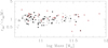 |
Fig. 1. Selection effects. Residuals from the mean size–mass relation vs. mass. Open and closed points refer to galaxies below and above z = 1, respectively. Galaxies with missing r80 sizes are indicated by a cross. |
3. Results
3.1. r80-mass scaling
Table 1 lists id, r80, concentration C85, and applied PSF correction to r80 of the 128 early-type galaxies studied in this work. Coordinates, masses, and half-light radii are listed in Paper I. Figure 2 shows the r80-mass relation at various redshifts.
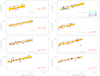 |
Fig. 2. Mass-size relation of red-sequence early-type cluster galaxies. The yellow shading indicates the 68% uncertainty (posterior higher density) and the dashed blue line indicates the corridor ±1σ range around the mean model. The solid gray line (not visible in the z = 0.17 panel) shows the z = 0.17 mass-size relation. At z < 1 points with black contours are spectroscopically confirmed galaxies. The horizontal dotted line indicates the PSF full width at half maximum (FWHM, below the minimal size at low redshifts). Sizes are corrected for (negligible) PSF blurring effects. |
Id, r80, concentration, and applied PSF corrections.
The scatter at a given mass is clearly non-Gaussian, at least because of the presence of few outliers (e.g., the most massive galaxy of the cluster at z = 0.44 in Fig. 2). Therefore, we fit the mass-size relation modeling the scatter around it with a Student-t distribution with ten degrees of freedom to limit the impact of outliers, as already done in Andreon (2012) to model the metallicity scatter. In the fit, we also leave the slope free in order to allow different evolutions at different masses and to de-weight log M/M⊙ ≫ 11 galaxies, because we want to focus on log M/M⊙ ∼ 11 galaxies (see Paper I for technical details). Fit results are listed in Table 2 and displayed in Fig. 2. Figure 2 also shows the z = 0.17 mass-size relation as solid gray line. As for the more studied r50 sizes, galaxies become smaller with increasing redshift.
Results of the various y = βx + α fits with scatter given by a Student-t distribution with scale s, before corrections for selection effects.
The mean size at log M/M⊙ = 11 after (minor) selection-effect corrections is shown in Fig. 3 as a function of redshift. To quantify the possible decrease in mean size with redshift, we fit a linear relation with uniform priors on intercept and angle. We find:

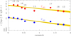 |
Fig. 3. Sizes at log M/M⊙ = 11 vs. redshift. Red and blue points are r80 and r50 sizes, respectively. The number above the points indicates the number of galaxies. The solid line and shading show the fitted relation and its 68% uncertainty (posterior highest density interval). |
as depicted in Fig. 3. The found redshift dependence, −0.11 ± 0.02, is less than 1σ away from that found for the half-light radius, −0.13 ± 0.02 in Andreon (2018), also depicted in Fig. 3; this indirectly suggests a minor, at most, evolution in concentration.
Figure 4 compares the scatter around the mass-size relation when using both r50 and r80. There is a weak indication2 for a tighter mass-size relation when using r80 compared to when using r50, but more data are needed to strengthen the evidence3.
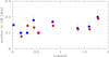 |
Fig. 4. Scatter around the size-mass relation vs. redshift. Red and blue points refer to r80 and r50 sizes, respectively. Scatter is computed from Student-t scale s as |
3.2. Concentration-mass scaling
Figure 5 shows the C85-mass relation of red-sequence early-type galaxies. As for the r80-mass relation, we adopted a Student-t distribution with ten degrees of freedom to model the scatter around the mean relation. In the fit, we also left the slope free so as to not force the same evolution at different masses and to de-weight log M/M⊙ ≫ 11 galaxies. One extreme outlier, the most massive galaxy in the z = 1.60 sample, is flagged by hand because, lying at masses unsampled by other data, it severely affects the derived slope. Fit results are listed in Table 2 and also displayed in Fig. 5. The mean concentration index at log M/M⊙ = 11 is shown in Fig. 6 as a function of the redshift, and fitted as was done for the mean r80 − z relation. We find:

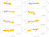 |
Fig. 5. Concentration-mass relation of red-sequence early-type cluster galaxies. The yellow shading indicates the 68% uncertainty (posterior higher density), the dashed blue corridor indicates a ±1σ range around the mean model. Concentrations are corrected for (negligible) PSF blurring effects. |
as depicted in Fig. 6. At a fixed mass, early-type galaxies on the red sequence have not changed concentration in the last 10 Gyr.
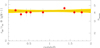 |
Fig. 6. Concentration at log M/M⊙ = 11 vs. redshift. The solid line and shading show the fitted relation and its 68% uncertainty (posterior highest-density interval). |
The right ordinates of Figs. 5 and 6 show approximated Sersic indices corresponding to the measured concentration index. These are derived from the growth curve of simulated galaxies with Sersic profiles for illustrative purposes only. In the presence of a background, the determination of C85 and Sersic index nsersic depends on the precise way the background is estimated for galaxies with large values of C85 or Sersic index. For example, estimating the background at three times the effective radius leads to a strongly biased determination of concentration and Sersic index of nser ≳ 4 (because r80 ≈ 3r50). Our C85 − nsersic conversion assumes Sersic profiles and that the background is measured at ≈7r50. We always use C85 in our analyses and the conversion to the Sersic index is only shown in our figures for a qualitative appreciation of the sensitivity of our measurement on a scale commonly used.
Figure 7 shows the scatter in concentration as a function of redshift. The scatter is about 15% and quite constant with redshift, indicating that the population spread is largely time-independent.
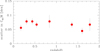 |
Fig. 7. Scatter around the concentration-mass relation vs. redshift. Scatter is computed from Student-t scale s as |

4. Summary and discussion
4.1. Lexical preamble
As emphasized in the introduction and sketched in Fig. 8, (a) concentration is a measure orthogonal to size and (b) compactness is a measure of the form of the profile; exponential profiles have smaller values of the index C85 than de Vaucouleurs profiles, no matter the size, compactness, or mass of the two compared profiles. The two terms should not be interchanged; for example, high redshift galaxies are not more concentrated because they are smaller (when, for example, they have the same Sersic or C85 index). Furthermore, the concept of compactness assumes the existence of a spread in size at a fixed mass; a system is not compact because its effective radius is small, but because there are other larger galaxies, that is to say there is a spread in size4. For this reason we modeled the spread vertically in the mass-size plane, instead of, for instance, studying the (dis)appearance of compact objects by defining compactness using an absolute size, or density, threshold. The latter choice mixes the target measurement with a variation in the scatter at a given mass and with the evolution of the mean relation5. Finally, measurements performed on observational data are made at a fixed mass (or a fixed number density, or at the fixed quantity that is used for measurements), and this should be kept in mind when interpreting the results. We can consider, for example, the universe simulated in Naab et al. (2009) formed by early-type galaxies that grow in size by a factor of 2.6 while their mass growth is 0.3 dex between z = 2 to z = 0. We can assume that the mass-size relation has a slope of ∼0.5, in agreement with observations. Some studies would have concluded that galaxies were 0.4 dex (=log2.6) smaller at high redshift. Other studies would have instead reported that galaxies are 0.25 dex smaller at high redshift at a fixed mass. In fact, galaxies that are 0.3 dex more massive have 0.15 dex larger sizes because of the mass-size relation, and therefore the growth at a fixed mass is 0.25 dex. In short, evolution is partially along the mass-size relation. Some studies would have suggested that in the above universe galaxies were compact at z = 2, but since there is no spread in size at a fixed mass in that universe, no galaxy is compact whatever its redshift may be. At most, z = 2 galaxies might be called small compared to present-day standards.
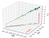 |
Fig. 8. Sketch view, with arbitrary points, of the mass-size-concentration space occupied by galaxies. |
To summarize, the orthogonal concepts of compactness and concentration must not be confused; compactness deals with size and needs a spread at fixed mass, while concentration deals with the curvature of the surface brightness profile. Our concentration index is sensitive to the curvature outside the effective radius by the way it is defined and because of the ∼1 kpc resolution of the data at high redshift. Instead, a hypothetical concentration index involving the 20% flux radius would require the measurement of fluxes in apertures smaller than the WFC3 pixel size at all masses at high redshift.
4.2. Summary of main results
Using an almost random sampling of a mass-limited sample formed by 128 morphologically early-type galaxies in clusters with log M/M⊙ ≳ 10.7 spanning the wide range 0.17 < z < 1.81, we find that in the last 10 Gyr both half-light and 80% light sizes increase by a factor of 1.7, and that concentration stays constant within 2%, that is to say the size growth of early-type galaxies in cluster environments proceeds at the same pace at both radii. The scatter around the mean relation measures the amount of variability, from system to system, of the amount of dissipation that leads to the observed galaxy. The constancy of the scatter around the size-mass relation with redshift (Fig. 4) implies that dissipation does not vary greatly with epoch.
4.3. Morphological sample selection is key
Unlike most published mass-size relations, our sample is morphologically selected. Only one-third of passive galaxies have an early-type morphology (Paper I). Indeed, passive galaxies are formed by a mix of early-type galaxies, recently quenched galaxies, and dusty star-forming galaxies (Williams et al. 2009; Moresco et al. 2013; Carollo et al. 2013; Paper I; Andreon 2018) and splitting this composite sample into more homogeneous parts is key to discriminate size or concentration evolution from a change of the morphological mix. In fact, morphological classification allowed De Propris et al. (2016) to properly interpret the measured apparent concentration change.
In literature, the Sersic index is often used to select the sample of early-type galaxies (e.g., Newman et al. 2014; De Propris et al. 2016; Strazzullo et al. 2010 for clusters; for galaxies in the field this is the rule). Our sample is morphologically selected and as such avoids the complications of studying the evolution in concentration of a concentration-selected sample; if galaxies of a given morphological type with a given value of concentration are missing, it is because Nature does not produce them.
4.4. Size growth: intrinsic vs. entirely due to a mass growth
Since we find a size growth at fixed mass, and size itself depends on mass, a natural question is to what extent the measured size growth is just mirroring a possible mass growth. Between the z = 2 to z = 0, stellar mass is barely growing, if at all. Mass and luminosity function determinations of early-type galaxies in cluster concur to find a non-evolving massive end, with upper limits of ∼0.1 dex change between z = 2 and z = 0 (Andreon 2006, 2012; Andreon et al. 2014 and references therein), given some assumptions, such as which synthesis population model and age are used (see for example Andreon et al. 2014). A neglected 0.1 dex mass change would spuriously bias the evolution at fixed mass by 0.05 dex in size because of the ∼0.5 slope of the mass-size relation. However, the observed evolution at a fixed mass is 0.22 dex, well beyond the effects of a hypothetically neglected 0.1 dex evolution in mass. To observe a spurious 0.22 dex evolution at fixed mass, we would need a mass evolution four times larger than what is allowed by observations.
4.5. The lack of scenario explaining all the observations
While both the mean r80 or r50 sizes change by a factor of 1.7 (see Sect. 3.1), concentration stays constant (within 2%, Sect. 3.2). The spread in concentration is small (∼15%) and constant (Fig. 7). Now we consider some unsuccessful attempts to find a physical mechanism producing trends in agreement with the observations.
First, progenitor bias has been already discussed and discarded in Paper I. Figure 9 reiterates the point, this time using ages of Coma galaxies from Harrison et al. (2010), chosen because they were used by Saracco et al. (2020) to claim the existence of a progenitor bias. Galaxies below, on, and above the mass-size relations have much the same median age and distribution of ages. To induce a bias in the intercept of the mass-size, there should instead be a trend in age as a function of size residuals at a fixed mass (abscissa), not visible in Fig. 9, independently confirming the similar result in Paper I using Smith et al. (2012) ages.
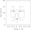 |
Fig. 9. Age distribution of Coma early-type galaxies small, average, and large for their mass, respectively. The plot is a standard box-whisker; the vertical box width delimits the 1st and 3rd quartile, while the median (2rd quartile) is indicated by the blue horizontal segment inside the box. The horizontal box width gives the full x range of each bin, while the error bars reach the minimum and maximum in the ordinate. Observed ages can be older than the Universe age because of errors. |
Second, truncation by the cluster halo should, at first glance, affect r80 more than the inner radius r50, and therefore should decrease the value of the C85 index. Given that we instead observed increasing sizes and constant values of C85, truncation seems to be excluded by the data. Furthermore, baryons are distributed in a more compact way than dark matter in galaxy halos (Limousin et al. 2009) and therefore truncation seems to be excluded a priori, as well as by observations.
Third, mergers, either major or minor, seems to be excluded because major mergers mostly increase mass, whereas minor mergers mainly change concentration, at least in simple settings. Idealized simulations of galaxies living outside a massive halo (cluster) in a non-cosmological setting predict an inside-out growth accompanied by a mass growth (Nipoti et al. 2003; Naab et al. 2009; Hilz et al. 2013), with amplitudes depending on which publication is considered and on whether the accretion is minor or major, unlike what we observe for galaxies. Moving to cosmological simulations, our negligible evolution of concentration with cosmic time of early-type galaxies in cluster is instead in line with the results of numerical simulation of massive galaxies in Tacchella et al. (2019). However, size and mass evolution of simulated galaxies grossly mismatch the observed evolution, perhaps due to differences in environments between simulated and observed galaxies. Overall, it is unclear whether results obtained on simulations of galaxies outside large massive halos, either idealized or cosmological, can be applied for galaxies inside a large massive halo. Nevertheless, Tacchella et al. (2019) simulations show that it is possible to change galaxy sizes without changing the galaxy concentration, though still changing the galaxy mass.
A meaningful comparison that allows us to shed light on which mechanisms are operating in galaxy clusters would require cosmological simulations of galaxies in massive clusters. However, current simulations either do not have the < 1 kpc resolution for measuring galaxy size and concentration, or do not sample volumes large enough to include rich galaxy clusters. There is the notable exceptions of a few cluster re-simulations, such as C-EAGLE (Barnes et al. 2017), which, however, do not have any published predictions.
4.6. A potential bias on estimate of structure evolution
With rare exceptions, the half-light, or half-mass, radius is identified with the galaxy size in literature, and its evolution is interpreted as the evolution of the whole galaxy structure. The inferred evolution of galaxy structure, commonly derived using r50 sizes, seems not to be biased by the arbitrary choice of using half-light radii, at least for the radii considered in this work and for early-type galaxies in cluster.
4.7. Comparison with previous works
Compared to color gradient measurements (e.g., De Propris et al. 2015; Chan et al. 2016; Ciocca et al. 2017), our study, measuring the relative rate at which the main body and the outskirts are built, has the advantage of directly assessing the relative structure build-up. In fact, under the optimistic assumption that color gradients are only sensitive to age differences, a given color gradient may imply a huge mass accretion or merging, or not at all, depending on the unknown age difference between accreted and already-present stellar populations. For a similar reason, spatially unresolved spectroscopy (e.g. Saracco et al. 2020; Stockmann et al. 2020; Matharu et al. 2020) is inadequately informative about the relative build-up of the central and outer parts of the galaxies; spatially-unresolved spectra measure stellar ages, averaged over a large portion of the galaxy, not assembly time of the galaxy parts.
To our best knowledge, there are no directly comparable studies on the evolution of concentration of morphological early-type galaxies in clusters. Our study, measuring the relative growth of the galaxy main body and outskirts, goes beyond recent works on the mass-size relations of galaxies in clusters (Kelkar et al. 2015; Kuchner et al. 2017; Sweet et al. 2017; Morishita et al. 2017; Saracco et al. 2017; Matharu et al. 2019). Lacking published measurements of the r80-mass relation, of the concentration-mass relation, or of the concentration evolution, we cannot compare relations derived by different authors or galaxy populations in clusters.
Even allowing the environment to be different, the literature is quite scarce. A precise comparison of the concentration evolution of related, yet different, classes of galaxies residing in different environments, such as Gu et al. (2019) vs. our study, is extremely difficult; it is difficult to constrain a problem with three covariates (population, environment, and amplitude of the progenitor bias) with two measurements. A meaningful comparison is easier at a fixed environment. Such a comparison is presented in a companion paper measuring concentration evolution in the field (Andreon, in prep.).
5. Conclusions
We measured the radii, including 80% of the light, of an almost random sampling of a mass-limited sample formed by 128 morphologically early-type galaxies in clusters with log M/M⊙ ≳ 10.7 spanning the wide range 0.17 < z < 1.81. We measured concentration by combining it with the half-light radius derived in Paper I. Because of the adopted non-parametric estimate of concentration, it focuses on the outer region of the galaxy and is insensitive to the profile inside the effective radius, unlike the Sersic index.
We found that concentration stays constant within 2% while both 50% and 80% light radii change by a factor of 1.7 from z = 2 to z = 0 at a fixed mass. We ruled out, for the second time, progenitor bias as a spurious source of size growth using an independent set of ages. We also ruled out mass growth as an entire source of size growth; to explain a 0.22 dex evolution in size, a 0.44 dex growth in mass is needed, while only at most 0.1 dex is allowed by mass function measurements.
Existing physical explanations proposed in the literature are unable to consistently explain the changing radii at a fixed mass while keeping concentration constant when mass evolution is negligible, which call for adopting or performing cluster simulations in a cosmological setting with a sufficient resolution (better than 1 kpc, to resolve the effective radius) to identify the physical mechanism affecting the galaxy structure.
Paper I also included the Coma cluster. The historical data of this cluster seem to be no longer readable on current devices, while more recent observations (e.g., Adami et al. 2006) are inadequate for our purposes because the background subtraction is too aggressive, leading to over-subtraction of the galaxy’s outer regions (Andreon 2002) and an underestimate of r80 and of the concentration index. Therefore, the current work omitted this cluster altogether.
Acknowledgments
SA thanks the anonymous referee for his/her valuable report, S. Tacchella for providing their concentrations updated for the C85 index, C. Nipoti for useful comments, P. Saracco for useful discussions, and C. Bernasconi, B. Garilli, C. Giorgieri, and M. Marelli for efforts in recovering data saved 25 years ago in a nowadays obsolete device. It’s a pleasure to thank the late Raymond Michard, whose original code turned out to be easy to modify to compute the concentrations used in this work.
References
- Adami, C., Picat, J. P., Savine, C., et al. 2006, A&A, 451, 1159 [NASA ADS] [CrossRef] [EDP Sciences] [MathSciNet] [Google Scholar]
- Andreon, S. 2002, A&A, 382, 495 [NASA ADS] [CrossRef] [EDP Sciences] [Google Scholar]
- Andreon, S. 2006, A&A, 448, 447 [NASA ADS] [CrossRef] [EDP Sciences] [Google Scholar]
- Andreon, S. 2010, MNRAS, 407, 263 [NASA ADS] [CrossRef] [Google Scholar]
- Andreon, S. 2012, A&A, 546, A6 [NASA ADS] [CrossRef] [EDP Sciences] [Google Scholar]
- Andreon, S., Newman, A. B., Trinchieri, G., et al. 2014, A&A, 565, A120 [NASA ADS] [CrossRef] [EDP Sciences] [Google Scholar]
- Andreon, S. 2018, A&A, 617, A53 [NASA ADS] [CrossRef] [EDP Sciences] [Google Scholar]
- Andreon, S., Dong, H., & Raichoor, A. 2016, A&A, 593, A2 (Paper I) [NASA ADS] [CrossRef] [EDP Sciences] [Google Scholar]
- Barnes, D. J., Kay, S. T., Bahé, Y. M., et al. 2017, MNRAS, 471, 1088 [NASA ADS] [CrossRef] [Google Scholar]
- Bruzual, G., & Charlot, S. 2003, MNRAS, 344, 1000 [NASA ADS] [CrossRef] [Google Scholar]
- Caon, N., Capaccioli, M., & D’Onofrio, M. 1993, MNRAS, 265, 1013 [NASA ADS] [CrossRef] [Google Scholar]
- Carollo, C. M., Bschorr, T. J., Renzini, A., et al. 2013, ApJ, 773, 112 [NASA ADS] [CrossRef] [Google Scholar]
- Chan, J. C. C., Beifiori, A., Mendel, J. T., et al. 2016, MNRAS, 458, 3181 [NASA ADS] [CrossRef] [Google Scholar]
- Ciocca, F., Saracco, P., Gargiulo, A., et al. 2017, MNRAS, 466, 4492 [Google Scholar]
- de Vaucouleurs, G. 1977, Evol. Galaxies Stellar Popul., 43, [Google Scholar]
- De Propris, R., Bremer, M. N., & Phillipps, S. 2015, MNRAS, 450, 1268 [NASA ADS] [CrossRef] [Google Scholar]
- De Propris, R., Bremer, M. N., & Phillipps, S. 2016, MNRAS, 461, 4517 [CrossRef] [Google Scholar]
- Fraser, C. W. 1972, Observatory, 92, 51 [Google Scholar]
- Graham, A. W., Erwin, P., Caon, N., et al. 2001, ApJ, 563, L11 [NASA ADS] [CrossRef] [Google Scholar]
- Gu, Y., Fang, G., Yuan, Q., et al. 2019, ApJ, 884, 172 [CrossRef] [Google Scholar]
- Gu, Y., Fang, G., Yuan, Q., et al. 2020, PASP, 132, 054101 [CrossRef] [Google Scholar]
- Harrison, C. D., Colless, M., Kuntschner, H., et al. 2010, MNRAS, 409, 1455 [CrossRef] [Google Scholar]
- Hilz, M., Naab, T., & Ostriker, J. P. 2013, MNRAS, 429, 2924 [NASA ADS] [CrossRef] [Google Scholar]
- Kelkar, K., Aragón-Salamanca, A., Gray, M. E., et al. 2015, MNRAS, 450, 1246 [NASA ADS] [CrossRef] [Google Scholar]
- Kuchner, U., Ziegler, B., Verdugo, M., et al. 2017, A&A, 604, A54 [NASA ADS] [CrossRef] [EDP Sciences] [Google Scholar]
- Limousin, M., Sommer-Larsen, J., Natarajan, P., et al. 2009, ApJ, 696, 1771 [NASA ADS] [CrossRef] [Google Scholar]
- Matharu, J., Muzzin, A., Brammer, G. B., et al. 2019, MNRAS, 484, 595 [CrossRef] [Google Scholar]
- Matharu, J., Muzzin, A., Brammer, G. B., et al. 2020, MNRAS, 493, 6011 [CrossRef] [Google Scholar]
- Miller, T. B., van Dokkum, P., Mowla, L., et al. 2019, ApJ, 872, L14 [NASA ADS] [CrossRef] [Google Scholar]
- Moresco, M., Pozzetti, L., Cimatti, A., et al. 2013, A&A, 558, A61 [NASA ADS] [CrossRef] [EDP Sciences] [Google Scholar]
- Morishita, T., Abramson, L. E., Treu, T., et al. 2017, ApJ, 835, 254 [NASA ADS] [CrossRef] [Google Scholar]
- Naab, T., Johansson, P. H., & Ostriker, J. P. 2009, ApJ, 699, L178 [NASA ADS] [CrossRef] [Google Scholar]
- Newman, A. B., Ellis, R. S., Andreon, S., et al. 2014, ApJ, 788, 51 [NASA ADS] [CrossRef] [Google Scholar]
- Nipoti, C., Londrillo, P., & Ciotti, L. 2003, MNRAS, 342, 501 [NASA ADS] [CrossRef] [Google Scholar]
- Patel, S. G., Holden, B. P., Kelson, D. D., et al. 2012, ApJ, 748, L27 [NASA ADS] [CrossRef] [Google Scholar]
- Raichoor, A., & Andreon, S. 2012, A&A, 543, A19 [NASA ADS] [CrossRef] [EDP Sciences] [Google Scholar]
- Salpeter, E. E. 1955, ApJ, 121, 161 [Google Scholar]
- Saracco, P., Gargiulo, A., Ciocca, F., et al. 2017, A&A, 597, A122 [NASA ADS] [CrossRef] [EDP Sciences] [Google Scholar]
- Saracco, P., Gargiulo, A., La Barbera, F., et al. 2020, MNRAS, 491, 1777 [CrossRef] [Google Scholar]
- Smith, R. J., Lucey, J. R., & Carter, D. 2012, MNRAS, 421, 2982 [NASA ADS] [CrossRef] [Google Scholar]
- Strazzullo, V., Rosati, P., Pannella, M., et al. 2010, A&A, 524, A17 [NASA ADS] [CrossRef] [EDP Sciences] [Google Scholar]
- Stockmann, M., Toft, S., Gallazzi, A., et al. 2020, ApJ, 888, 4 [CrossRef] [Google Scholar]
- Sweet, S. M., Sharp, R., Glazebrook, K., et al. 2017, MNRAS, 464, 2910 [NASA ADS] [CrossRef] [Google Scholar]
- Tacchella, S., Diemer, B., Hernquist, L., et al. 2019, MNRAS, 487, 5416 [CrossRef] [Google Scholar]
- van Dokkum, P. G., Whitaker, K. E., Brammer, G., et al. 2010, ApJ, 709, 1018 [NASA ADS] [CrossRef] [Google Scholar]
- Williams, R. J., Quadri, R. F., Franx, M., van Dokkum, P., & Labbé, I. 2009, ApJ, 691, 1879 [NASA ADS] [CrossRef] [Google Scholar]
All Tables
Results of the various y = βx + α fits with scatter given by a Student-t distribution with scale s, before corrections for selection effects.
All Figures
|
Fig. 1. Selection effects. Residuals from the mean size–mass relation vs. mass. Open and closed points refer to galaxies below and above z = 1, respectively. Galaxies with missing r80 sizes are indicated by a cross. |
| In the text | |
|
Fig. 2. Mass-size relation of red-sequence early-type cluster galaxies. The yellow shading indicates the 68% uncertainty (posterior higher density) and the dashed blue line indicates the corridor ±1σ range around the mean model. The solid gray line (not visible in the z = 0.17 panel) shows the z = 0.17 mass-size relation. At z < 1 points with black contours are spectroscopically confirmed galaxies. The horizontal dotted line indicates the PSF full width at half maximum (FWHM, below the minimal size at low redshifts). Sizes are corrected for (negligible) PSF blurring effects. |
| In the text | |
|
Fig. 3. Sizes at log M/M⊙ = 11 vs. redshift. Red and blue points are r80 and r50 sizes, respectively. The number above the points indicates the number of galaxies. The solid line and shading show the fitted relation and its 68% uncertainty (posterior highest density interval). |
| In the text | |
|
Fig. 4. Scatter around the size-mass relation vs. redshift. Red and blue points refer to r80 and r50 sizes, respectively. Scatter is computed from Student-t scale s as |
| In the text | |
|
Fig. 5. Concentration-mass relation of red-sequence early-type cluster galaxies. The yellow shading indicates the 68% uncertainty (posterior higher density), the dashed blue corridor indicates a ±1σ range around the mean model. Concentrations are corrected for (negligible) PSF blurring effects. |
| In the text | |
|
Fig. 6. Concentration at log M/M⊙ = 11 vs. redshift. The solid line and shading show the fitted relation and its 68% uncertainty (posterior highest-density interval). |
| In the text | |
|
Fig. 7. Scatter around the concentration-mass relation vs. redshift. Scatter is computed from Student-t scale s as |
| In the text | |
|
Fig. 8. Sketch view, with arbitrary points, of the mass-size-concentration space occupied by galaxies. |
| In the text | |
|
Fig. 9. Age distribution of Coma early-type galaxies small, average, and large for their mass, respectively. The plot is a standard box-whisker; the vertical box width delimits the 1st and 3rd quartile, while the median (2rd quartile) is indicated by the blue horizontal segment inside the box. The horizontal box width gives the full x range of each bin, while the error bars reach the minimum and maximum in the ordinate. Observed ages can be older than the Universe age because of errors. |
| In the text | |
Current usage metrics show cumulative count of Article Views (full-text article views including HTML views, PDF and ePub downloads, according to the available data) and Abstracts Views on Vision4Press platform.
Data correspond to usage on the plateform after 2015. The current usage metrics is available 48-96 hours after online publication and is updated daily on week days.
Initial download of the metrics may take a while.