| Issue |
A&A
Volume 640, August 2020
|
|
|---|---|---|
| Article Number | A79 | |
| Number of page(s) | 7 | |
| Section | Galactic structure, stellar clusters and populations | |
| DOI | https://doi.org/10.1051/0004-6361/201937279 | |
| Published online | 14 August 2020 | |
Taking apart the dynamical clock
Fat-tailed dynamical kicks shape the blue straggler star bimodality
1
INAF, Osservatorio Astronomico di Padova, vicolo dell’Osservatorio 5, 35122 Padova, Italy
e-mail: mario.pasquato@oapd.inaf.it
2
INFN – Sezione di Padova, Via Marzolo 8, 35131 Padova, Italy
3
Dipartimento di Fisica e Astronomia & CSDC, Università di Firenze, via Sansone 1, 50019 Sesto Fiorentino, Italy
e-mail: pierfrancesco.dicintio@unifi.it
4
INFN – Sezione di Firenze, via Sansone 1, 50019 Sesto Fiorentino, Italy
Received:
6
December
2019
Accepted:
1
May
2020
Context. In globular clusters (GCs), blue straggler stars (BSS) are heavier than the average star, so dynamical friction strongly affects them. The radial distribution of BSS, normalized to a reference population, appears bimodal in a fraction of Galactic GCs, with a density peak in the core, a prominent zone of avoidance at intermediate radii, and again higher density in the outskirts. The zone of avoidance appears to be located at larger radii the more relaxed the host cluster, acting as a sort of dynamical clock.
Aims. We use a new method to compute the evolution of the BSS radial distribution under dynamical friction and diffusion.
Methods. We evolve our BSS in the mean cluster potential under dynamical friction plus a random fluctuating force, solving the Langevin equation with the Mannella quasi symplectic scheme. This is a new simulation method that is much faster and simpler than direct N-body codes, but retains their main feature: diffusion powered by strong, if infrequent, kicks.
Results. We compute the radial distribution of initially unsegregated BSS normalized to a reference population as a function of time. We trace the evolution of its minimum, corresponding to the zone of avoidance. We compare the evolution under kicks extracted from a Gaussian distribution to that obtained using a Holtsmark distribution. The latter is a fat-tailed distribution which correctly models the effects of close gravitational encounters. We find that the zone of avoidance moves outwards over time, as expected based on observations, only when using the Holtsmark distribution. Thus, the correct representation of near encounters is crucial to reproduce the dynamics of the system.
Conclusions. We confirm and extend earlier results that showed how the dynamical clock indicator depends on dynamical friction and on effective diffusion powered by dynamical encounters. We demonstrated the high sensitivity of the clock to the details of the mechanism underlying diffusion, which may explain the difficulties in reproducing the motion of the zone of avoidance across different simulation methods.
Key words: blue stragglers / methods: analytical / methods: numerical / globular clusters: general
© ESO 2020
1. Introduction
Blue straggler stars (BSS) were first observed by Sandage (1953) as a blueward and brighter continuation of the main sequence in the globular cluster (GC) M3, and have since been found in all GCs in the Milky Way (Piotto et al. 2004; Ferraro et al. 2020, and references therein). BSS in dense stellar systems such as GCs have typical masses mBSS of the order of twice the mean stellar mass m* in the host cluster and are born either through mass transfer in close binary stars (McCrea 1964) or via direct stellar collisions (Hills & Day 1976). More recently, it has been suggested that BSS may also form via hierarchical merging induced by the Lidov–Kozai mechanism (Lidov 1962; Kozai 1962, see also Fabrycky & Tremaine 2007) in triple systems (see e.g. Perets & Fabrycky 2009; Boffin et al. 2015; Antonini et al. 2016).
Each formation channel of BSS is favoured in different regions of the host GC. For example, the dense core allows more collisions-induced BSS mergers (Verbunt et al. 1987). Early observational studies revealed a bimodal distribution of the BSS population in GCs (Ferraro et al. 1993; Zaggia et al. 1997), which was interpreted as evidence that the two channels are simultaneously active, and Monte Carlo simulations confirmed this interpretation (Mapelli et al. 2004, 2006), as did scaling laws for the number of BSS with GC structural parameters (Davies et al. 2004). As later observational efforts increased the sample of GCs with a well-observed BSS radial distribution, including cases where no bimodality was present (e.g. Ferraro et al. 2006; Dalessandro et al. 2008), it became apparent that the observed BSS bimodality is closely linked to the dynamical relaxation of the host GC, to the point that it can be used as a sort of dynamical clock to measure the evolutionary stage of a GC (Ferraro et al. 2012). This finding, together with the proportionality of the BSS number with GC core mass (e.g. Knigge et al. 2009) qualitatively supports a scenario where BSS originate from primordial binaries for the most part, as is also suggested by much more recent direct observations (Giesers et al. 2019; Gosnell et al. 2019).
However, a qualitative agreement is not enough to rule out the direct-collision channel (also supported by earlier hydrodynamical simulations by Lombardi et al. 1996), which could still bring a significant contribution to the BSS population in GC cores. In addition, there have been recent claims of observational evidence of possible ternary mergers as the origin of BSS (Andrews et al. 2016; Kohler et al. 2018) as well as evidence of BSS with white dwarfs companions (Ekanayake & Wilhelm 2018; N et al. 2020). A precise quantitative prediction of the mass-transfer BSS distribution as a function of time would allow us to obtain, by subtraction from the observations, the number of direct-collision BSS present in cores, if any.
To be able to make this sort of clear-cut quantitative predictions, a clear understanding of the physics underlying the dynamical clock is needed. This is necessary for example to understand whether the initial conditions of a simulation are located in the correct region of parameter space needed to obtain the observed formation and outward motion of the BSS distribution minimum, and whether the results of a small-scale simulation can be scaled up to describe a larger system. Realistic simulation studies based on direct N-body simulations (Ferraro et al. 2012; Alessandrini et al. 2014, 2016; Miocchi et al. 2015; Alessandrini & Cosmic-Lab Team 2016) or state-of-the-art Monte Carlo simulations (Hypki & Giersz 2013, 2017; Sollima & Ferraro 2019), while valuable for a direct comparison with observations in the spirit of saving the phenomena, are less concerned with gaining this kind of understanding. In a previous paper, Pasquato et al. (2018) made some progress towards this goal by showing the following:
-
to form a minimum, i.e. to obtain a bimodal BSS distribution, dynamical friction is a necessary ingredient;
-
to move the minimum to larger radii over time, an effective diffusion mechanism is needed;
-
to obtain a bimodal distribution with a minimum that moves outwards over time, dynamical friction and diffusion should be balanced within a narrow range.
The last condition in particular is not necessarily trivial to achieve within a simulation, but in real systems it stems naturally from fundamental fluctuation-dissipation relations that connect dynamical friction and diffusion, which are ultimately two aspects of the same phenomenon (Kandrup 1980, 1981).
Pasquato et al. (2018) was based on a one-dimensional Brownian motion model, with particles representing the average radial positions of stars over their orbits. The limitations of this model coincide with the limitations of the intuitive picture of BSS sitting undisturbed at large radii until the zone of avoidance (Mapelli et al. 2004) reaches the scale radius of their orbit as dynamical relaxation takes place; specifically, in a three-dimensional system with non-circular orbits the radial position of stars changes on a timescale much shorter than the systems relaxation time simply because over an orbital period they move from the apocentre to the pericentre of their orbit and back. This was mentioned by Hypki & Giersz (2017) as the probable reason why the external regions of a simulated GC undergo a quick depletion of BSS even though the zone of avoidance has not yet reached them (see e.g. their Fig. 4).
In this work we solve a full three-dimensional model with stochastic differential equations for a population of non-interacting tracer particles representing the BSS evolving under the combined effect of the cluster potential, dynamical friction, and collisions with other stars. This method allows many BSS trajectories to be run without interfering with the cluster dynamics (as they get kicks from the cluster stars, but they do not give any feedback to them), so that better statistics can be obtained, while avoiding triggering the Spitzer (1969) instability.
Moreover, at variance with other stochastic schemes based on the evolution of probability density functions (PDFs) for the particles phase-space coordinates, with the Fokker–Planck equation (see Rosenbluth et al. 1957 for the specific case of the 1/r2 force), frequently used to investigate the dynamics of black holes under the effect of gravitational encounters with stars (see e.g. Cohn & Kulsrud 1978; Chatterjee et al. 2002; Merritt 2015a,b; Darbha et al. 2019), our approach can be easily tuned to include a mass spectrum (Ciotti et al. 2010), orbital anisotropy, or the effect of a time-dependent external potential, among others.
This paper is structured as follows. In Sect. 2 we present the numerical scheme to solve the Langevin equations for the population of BSS under the effect of the cluster potential and stellar collision. In Sect. 3 we present the results of our numerical calculations and discuss them in light of the observational results. Finally, in Sect. 4 we summarize and draw our conclusions.
2. Methods
We evolve an ensemble of non-interacting tracer particles (simulating the population of BSS) of equal mass mBSS, under the combined effect of the fixed star cluster mean field potential and stellar encounters resulting in a diffusion and friction process. Under these assumptions, the particle dynamics is described by the Langevin equation (see e.g. van Kampen 1992)

where ∇Φ is a smooth deterministic force field generated by the chosen spherical mass density, η is the dynamical friction coefficient (Chandrasekhar 1943, 1949), and F is a fluctuating force per unit mass, accounting for the granular nature of the underlying model. A similar approach has been used to treat different problems involving noise induced phase-space transport in the contexts of galactic dynamics (Habib et al. 1997; Pogorelov & Kandrup 1999; Kandrup et al. 2000; Terzic & Kandrup 2003; Sideris & Kandrup 2004) and charged particle beams (Sideris & Bohn 2004; Kandrup et al. 2004). More recently, Di Cintio et al. (2020) used this method to study the dynamics of the black holes at the centre of elliptical galaxies or star clusters, and finds a good agreement with simple direct N-body simulations.
In Eq. (1) the fixed gravitational potential Φ is generated by the usual Plummer (1911) density profile1
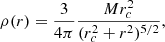
with total mass M and scale radius rc. The position-dependent dynamical friction coefficient (Miocchi et al. 2015) is defined as
where v = ||v||, lnΛ the Coulomb logarithm of the maximum-to-minimum impact parameter ratio bmax/bmin, and
is the velocity volume function. In the case of a Plummer model, the isotropic phase-space distribution function is written simply as f(r, v) = C[−Φ(r)−v2/2]7/2, where C is the normalization constant and  .
.
At variance with the one-dimensional “orbit gas” model of Pasquato et al. (2018), our model features isotropic kicks in three dimensions and we sample the norm F of the stochastic acceleration term in Eq. (1) from the Holtsmark (1919) distribution
![$$ \begin{aligned} H(F)=\frac{2}{\pi F}\int _0^\infty \exp \left[-\alpha (\xi /F)^{3/2}\right]\xi \sin (\xi )\mathrm{d}\xi , \end{aligned} $$](/articles/aa/full_html/2020/08/aa37279-19/aa37279-19-eq6.gif)
introduced originally in the context of plasma physics, and used for the first time in stellar dynamics by Chandrasekhar & von Neumann (1942, 1943) to study the fluctuations of the gravitational field acting on a test star. In Eq. (5) α = (4/15)(2πGm)3/2n is a normalization factor dependent on the number density n and stellar mass m. We note that in the original derivation by Chandrasekhar and von Neumann Eq. (5) is defined for an infinite and homogeneous system. In this work we assume a position-dependent Holtsmark distribution by substituting n*(r) = ρ(r)/m*, i.e. the local mean number density, in the normalization parameter α. However, for sufficiently flat-cored models the distribution of force fluctuations differs little from the Holtsmark distribution (see e.g. Bertiau & Roberts 1958).
Unfortunately, it is not possible to write Eq. (5) and its cumulative distribution in terms of simple functions. Moreover, except the first, the moments of the distribution are all singular2, which makes sampling the stochastic force term in Eq. (1) a delicate step.
In the limit of large F, the Holtsmark distribution (5) is closely approximated in polynomial form (see Hummer 1986) and, retaining only the leading term of the expansion, can be written as  . This expression, frequently used in numerical studies in the cosmological context (see Pietronero et al. 2002; Bottaccio et al. 2002, and references therein) still bears the same problems of its full integral form, being non-normalizable and with divergent standard deviation. Typically, in order to avoid a diverging cumulative distribution and diverging energy density of the fluctuating field (Kozlitin 2011), when sampling
  in numerical schemes one is forced to fix bona fide cut-offs at large and small F.
In the numerical simulations discussed in this work we use the integral representation of the Holtsmark distribution whose cumulative function
has been evaluated numerically on a unevenly spaced grid between 0 and a maximum force of the order of Gm*/β2, where β is the typical minimum impact parameter, which we set at 1/30 of the local mean inter-particle distance, corresponding to roughly the size of the Solar System at r ≈ 2rc for a star cluster of 106 stars with a scale radius rc of 1 pc.
In Fig. 1 we show the numerically recovered Holtsmark distribution of the intensity of the force fluctuations at different radii 0 ≤ r ≤ 2rc in a Plummer model, and the associated Maxwell-Boltzmann distributions peaking at the same F, resulting from assuming a three-dimensional Gaussian distribution of force fluctuations. As expected, the peaks of the Holtsmark and Gaussian distributions both drift towards lower forces as the radius increases. However, at all radii the Gaussian underestimates the contribution of strong kicks, corresponding to small impact parameters encounters between stars, with respect to the parent Holtsmark distribution.
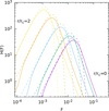 |
Fig. 1. Holtsmark (solid lines) and Maxwellian (dashed lines) distributions of the intensity of the gravitational force fluctuations at r/rc = 0 (purple), 0.5 (green), 1 (light blue), 1.5 (orange), and 2 (yellow) in a Plummer model. |
Equation (1) is an example of stochastic ordinary differential equation (see e.g. Gardiner 1994) for a single Brownian particle3 whose integration in general presents several technical issues due to the fluctuating nature of the stochastic force term F(r) (see e.g. San Miguel et al. 2000; Burrage et al. 2007, and references therein). In this work we use the quasi-symplectic method, introduced in Mannella (2004), which for the one-dimensional case reads
![$$ \begin{aligned}&x(t+\Delta t/2)=x(t)+\frac{\Delta t}{2}v(t)\nonumber \\&v(t+\Delta t)=c_2\left[c_1v(t)+\Delta t \nabla \Phi (x^\prime )+d_1 \tilde{F}(x^\prime ) \right]\nonumber \\&x(t+\Delta t)=x(t+\Delta t/2)+\frac{\Delta t}{2}v(t+\Delta t). \end{aligned} $$](/articles/aa/full_html/2020/08/aa37279-19/aa37279-19-eq10.gif)
In the equations above Δt is the fixed time-step (we usually take Δt ∼ 10−3tc, with  the crossing time of the system),
  is the normalized stochastic force (in this case, a random variable sampled from Eq. (5)), and
where ζ in the case of a delta correlated noise is fixed by the standard deviation of the distribution of F as

Since for the Holtsmark distribution the standard deviation and all higher moments are infinite, in our numerical scheme we use  of the full width at half maximum of the truncated distribution4 in place of σ. Given that the two distributions differ by several orders of magnitude for large F, we note that the results are left unchanged for other choices of the range 1/2, 3/2 of the full width at half maximum (see also Fig. 1). We also note that, for vanishing η and ζ, Eq. (7) yield back the standard Leapfrog method, which is second order and symplectic. Generalization to higher order schemes is also possible (see Mannella 2006; Burrage et al. 2007); however, for the scope of this paper we limited ourselves to the second-order method. Using a second-order method to solve Eq. (1) allows us to keep relatively short computational times even for a large number of test particles, while avoiding the contribution of the random force and dynamical friction a posteriori after a propagation step in the same fashion as Sigurdsson & Phinney (1995) for the interaction of Neutron stars with binaries in GCs.
In this study we have evolved 104 independent5 BSS with two values of mass mBSS = 1.5m* and 2m*, for 105tc. The background population of the GC is assumed in both cases to be 106 stars with equal masses m*.
The initial positions and velocities of the BSS are also drawn from the isotropic Plummer distribution. In order to evaluate the effects on the mass segregation of radial or tangential anisotropy, we also performed numerical integrations with the same parameters and initial positions of the BSS, but sampling their velocities from the two extreme cases of a purely radial or circular orbit distribution, as done for example in the case of pulsar binaries (Phinney & Sigurdsson 1991; Sigurdsson & Phinney 1995). In addition, to evaluate the importance of correctly modelling close encounters (represented by the fat tails of the Holstsmark distribution), we performed an additional set of numerical experiments using for the diffusion term in Eq. (1) a three-dimensional isotropic Gaussian distribution of force fluctuations (corresponding to a Maxwell–Boltzmann distribution of their modulus) instead of the Holtsmark distribution.
In each simulation set-up we extracted the projected distribution of the nBSS population normalized to the reference background population that was assumed to remain constant in time. In order to build the radial profile at a given time tp, we took the eight subsequent snapshots (taken one dynamical time apart from each other) and we merged them into one then pooling together all the stars projected along each of the three coordinate axes. This allows us to virtually increase the number of BSS in the sample by a factor 24, further reducing statistical fluctuations. We note that merging subsequent snapshots is justified because we are interested in the long-term dynamical evolution of the system, with respect to which snapshots separated by one dynamical time are essentially identical. The projected profiles were then binned in ten radial bins based on the quantiles of the Plummer density distribution, so that an equal number of reference stars would fall in each bin.
3. Results
In Figs. 2 and 3, we show the normalized projected radial BSS distribution at increasing dynamical times for a population of tracer particles representing the BSS in simulations using the Holtsmark and the three-dimensional Gaussian distributions of kicks, respectively. In all cases the distribution becomes markedly bimodal after a few hundred dynamical times tc. We note that in a typical globular cluster a dynamical (crossing) time corresponds to ≈105 yr, so the bimodality is established quite rapidly on the cosmological timescale.
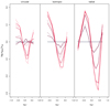 |
Fig. 2. Normalized BSS distribution nBSS/nref at t/tc = 0 (black), 500, 5000, 20 000, 50 000, and 80 000 (bright red) for a population of BSS with masses mBSS = 1.5m* (dashed lines) and mBSS = 2m* (solid lines), initially placed on purely circular orbits (left), extracted from a isotropic distribution (centre), and on purely circular orbits (right). |
We show the evolution of the position of the profile’s minimum, i.e. the centre of the zone of avoidance, as a function of time in Figs. 4–6. Remarkably, using Gaussian kicks fails to reproduce the motion of the minimum towards larger radii over time, while Holtsmark kicks reproduce it correctly, as can be seen by comparing the corresponding panels in Figs. 3 and 2. We note that this result holds for all the initial velocity distributions of the BSS explored here, namely isotropic, fully circular, and fully radial, so it is not dependent on the specific orbital eccentricity distribution. This was also confirmed by some additional test simulations (not shown here) where the BSS were initialized with different Osipkov–Merritt radially anisotropic profiles.
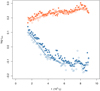 |
Fig. 4. Time evolution of the log radial position of the zone of avoidance for a population of BSS with masses mBSS = 1.5m* (empty circles) and mBSS = 2m* (filled circles), initially placed on randomly chosen isotropically distributed orbits. Time is measured in units of 104 dynamical crossing times. The orange circles refer to models employing a Holtsmark distribution of force fluctuations, while the blue circles refer to models where a three-dimensional Gaussian distribution of fluctuations was used. Plotted to guide the eye are a local polynomial regression (solid lines) fitted to the mBSS = 2m* zone of avoidance position for Holtsmark (orange) and Gaussian (blue) force kicks. Isotropic orbits are often assumed in most simple models of star clusters (e.g. King, Plummer); the results still hold even in the two extreme anisotropic scenarios where all orbits are circular (see Fig. 5) or radial (see Fig. 6). |
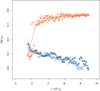 |
Fig. 5. Time evolution of the log radial position of the zone of avoidance for a population of BSS with masses mBSS = 1.5m* (empty circles) and mBSS = 2m* (filled circles), initially placed on purely circular orbits. Time is measured in units of 104 dynamical crossing times. The orange circles refer to models employing a Holtsmark distribution of force fluctuations, while the blue circles refer to models where a three-dimensional Gaussian distribution of fluctuations was used. Plotted to guide the eye are a local polynomial regression (solid lines) fitted to the mBSS = 2m* zone of avoidance position for Holtsmark (orange) and Gaussian (blue) force kicks. Circular and radial orbits (see Fig. 6) are two extreme cases considered to show that the results are robust to changes in the distribution of BSS orbital angular momenta. |
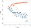 |
Fig. 6. Time evolution of the log radial position of the zone of avoidance for a population of BSS with masses mBSS = 1.5m* (empty circles) and mBSS = 2m* (filled circles), initially placed on purely radial orbits. Time is measured in units of 104 dynamical crossing times. The orange circles refer to models employing a Holtsmark distribution of force fluctuations, while the blue circles refer to models where a three-dimensional Gaussian distribution of fluctuations was used. Plotted to guide the eye are a local polynomial regression (solid lines) fitted to the mBSS = 2m* zone of avoidance position for Holtsmark (orange) and Gaussian (blue) force kicks. Radial and circular orbits (see Fig. 5) are two extreme cases considered to show that the results are robust to changes in the distribution of BSS orbital angular momenta. |
Curiously, regardless of the specific model of force fluctuations, we find that at large radii the BSS density drops quickly in the case of isotropic or purely radial distribution of orbits, while it takes longer in the case of circular orbits. This behaviour was discussed by Hypki & Giersz (2017), suggesting that it may be due to stars on elongated orbits suffering the effects of dynamical friction much faster than expected based merely on their instantaneous radial position. Our finding confirms this supposition.
In addition to the evolution of the minimum, distributions obtained under Gaussian and Holtsmark kicks also differ in the central region where the former rapidly produce a very strong peak, while the latter show a broader peak that increases slowly over time. In the outskirts, Gaussian kicks result in a slow drop in BSS density, while under Holtsmark kicks the reverse happens and density increases.
All these differences find a unified explanation in the fact that Gaussian kicks underestimate the intensity of diffusion because they do not correctly represent the effects of close encounters, as shown in Fig. 1. Underestimating diffusion allows most stars to fall to the core, forming a central peak and depleting the intermediate regions. As the central peak shrinks over time faster than the distribution in the outskirts gets eroded, the minimum moves towards the inside of the cluster. When two-body kicks are instead correctly accounted for by using the Holtsmark distribution, stars that fall to the core get kicked out, limiting the growth of the central peak and broadening it so that the minimum gets pushed to larger radii. Stars kicked out of the core are also responsible for the rise at large radii observed in the distributions obtained with the Holtsmark kicks. We note that Sigurdsson et al. (1994; but see also Mapelli et al. 2004) in an earlier attempt at modelling the radial BSS distribution also used a non-Gaussian distribution of Kicks, modelling the effect of triple collisions and inelastic scattering. Remarkably, the prominent peak at large radii in the relative BSS distribution is also recovered in their case.
4. Discussion and conclusions
Ferraro et al. (2012) have shown that the BSS zone of avoidance evolves in step with the relaxation of the host star cluster by comparing observational data with direct N-body simulations. While simplified, these simulations included a wide range of ingredients and their complex interactions. This is also true for N-body simulations performed later by the same group (Alessandrini et al. 2014; Miocchi et al. 2015) and even more for state-of-the-art Montecarlo simulations that include realistic stellar evolution (Hypki & Giersz 2013, 2017; Sollima & Ferraro 2019).
The motivation for our work was to do away with this complexity, pinpointing the minimal set of ingredients needed to reproduce the BSS distibution evolution revealed by observations. We confirm that, in addition to the smooth potential of the host GC, these ingredients are dynamical friction and diffusion, as found by Pasquato et al. (2018), but in the context of a full three-dimensional model where the stochastic differential equation describing dynamical evolution is solved numerically with diffusion arising from dynamical kicks modelled in a self-consistent way. Additionally, we determined that a correct modelling of these kicks is required to obtain an effective diffusion that reproduces the observed evolution of the radial position of the BSS zone of avoidance, showing how the dynamical clock depends on a delicate equilibrium between diffusion and friction. This may explain the apparent tension between the results of Hypki & Giersz (2017) and Ferraro et al. (2012)6: the formation of the zone of avoidance and its correct outward motion are possible only with the correct recipe for dynamical kicks. If we underestimate kicks (e.g. by assuming they are distributed normally, as shown in this work) not enough diffusion is present to push the BSS minimum outwards; if we overestimate them the diffusion is too strong and smoothes out the minimum. Except perhaps in a direct N-body model including the correct number of stars (i.e. over 106, which is at the limit of our current technological capabilities) there is in general no guarantee that the distribution of kicks is matched in any simulation setting, in particular in a Monte Carlo. Notwithstanding the large degree of simplification of our model (i.e. assuming the static and unrealistic Plummer density profile, neglecting stellar evolution and the binary nature of many BSS), the results presented in this work are encouraging and suggest that the dynamical clock is mainly related to the interplay between dynamical friction and fluctuations of the local gravitational field. A natural follow-up of our investigation would be the inclusion of a ‘live’ star cluster potential accounting for the effects of global dynamical evolution (i.e. core collapse and tidal compression due to the parent galaxy mass distribution) in order to shed some light on how much these collective processes influence the dynamical clock and its effectiveness as a way to estimate the age of GCs. At the moment, a systematic study using the more realistic King density profiles allowed to evolve by means of envelope equations for density and potential is underway. In addition, stochastic simulations involving the so-called multiparticle collision technique coupled with standard particle-mesh schemes (as recently done in plasma physics; see e.g. Di Cintio et al. 2017; Ciraolo et al. 2018) are underway. By using these methods it is therefore possible to compute the collective cluster potential self-consistently with a large number of particles (up to 108) while including the effects of stellar collisions with an operator that preserves locally the kinetic energy and angular and linear momentum of particles. These methods will allow us to study in more detail mass segregation problems with a larger number of particles than that attainable in direct N-body simulations via a scheme that is alternative to Monte Carlo at the same computational cost of the simpler Langevin simulations presented in this work.
The choice of the simple Plummer model, following Miocchi et al. (2015), is motivated mainly because it possesses analytic and relatively simple expressions for the potential and velocity dispersion, at variance with the more realistic King (1966) profile.
An approximated expression for the Holtsmark distribution with finite normalization and standard deviation can be obtained by substituting Eq. (5) for F ≥ F* with H1(F) = (α4/3L/F3)exp(−3F2/2α4/3), where  and F* is tuned so that the two expression mach for F = F* (see Petrovskaya 1986).

Particles representing the BSS are propagated separately according to Eq. (1) and their distribution does not affect the fixed GC potential.
In addition to the binning choices of the latter discussed by Hypki & Giersz (2017).
Acknowledgments
This project has received funding from the European Union’s Horizon 2020 research and innovation program under the Marie Skłodowska-Curie Grant agreement No. 664931. One of us (PFDC) wishes to thank the financing from MIUR-PRIN2017 project Coarse-grained description for non-equilibrium systems and transport phenomena (CO-NEST) n.201798CZL. We wish to thank Prof. Michela Mapelli for discussion and encouragement and the anonymous Referee for his/her important comments that improved the presentations of our results.
References
- Alessandrini, E., & Cosmic-Lab Team 2016, Mem. Soc. Astron. It., 87, 513 [Google Scholar]
- Alessandrini, E., Lanzoni, B., Miocchi, P., Ciotti, L., & Ferraro, F. R. 2014, ApJ, 795, 169 [NASA ADS] [CrossRef] [Google Scholar]
- Alessandrini, E., Lanzoni, B., Ferraro, F. R., Miocchi, P., & Vesperini, E. 2016, ApJ, 833, 252 [NASA ADS] [CrossRef] [Google Scholar]
- Andrews, J. J., Agüeros, M., Brown, W. R., et al. 2016, ApJ, 828, 38 [NASA ADS] [CrossRef] [Google Scholar]
- Antonini, F., Chatterjee, S., Rodriguez, C. L., et al. 2016, ApJ, 816, 65 [NASA ADS] [CrossRef] [Google Scholar]
- Bertiau, F. C., & Roberts, P. H. 1958, ApJ, 128, 130 [NASA ADS] [CrossRef] [Google Scholar]
- Boffin, H. M. J., Carraro, G., & Beccari, G. 2015, Ecol. Blue Straggler Stars, Vol, 413 [NASA ADS] [Google Scholar]
- Bottaccio, M., Amici, A., Miocchi, P., et al. 2002, Europhys. Lett., 57, 315 [NASA ADS] [CrossRef] [Google Scholar]
- Burrage, K., Lenane, I., & Lythe, G. 2007, SIAM J. Sci. Comput., 29, 245 [CrossRef] [Google Scholar]
- Chandrasekhar, S. 1943, ApJ, 97, 255 [NASA ADS] [CrossRef] [Google Scholar]
- Chandrasekhar, S. 1949, Rev. Mod. Phys., 21, 383 [NASA ADS] [CrossRef] [Google Scholar]
- Chandrasekhar, S., & von Neumann, J. 1942, ApJ, 95, 489 [NASA ADS] [CrossRef] [Google Scholar]
- Chandrasekhar, S., & von Neumann, J. 1943, ApJ, 97, 1 [NASA ADS] [CrossRef] [Google Scholar]
- Chatterjee, P., Hernquist, L., & Loeb, A. 2002, ApJ, 572, 371 [NASA ADS] [CrossRef] [Google Scholar]
- Ciotti, L. 2010, in American Institute of Physics Conference Series, eds. G. Bertin, F. de Luca, G. Lodato, R. Pozzoli, & M. Romé, AIP Conf. Ser., 1242, 117 [NASA ADS] [Google Scholar]
- Ciraolo, G., Bufferand, H., Di Cintio, P., et al. 2018, Contrib. Plasma Phys., 58, 457 [NASA ADS] [CrossRef] [Google Scholar]
- Cohn, H., & Kulsrud, R. M. 1978, ApJ, 226, 1087 [NASA ADS] [CrossRef] [Google Scholar]
- Dalessandro, E., Lanzoni, B., Ferraro, F. R., et al. 2008, ApJ, 681, 311 [NASA ADS] [CrossRef] [Google Scholar]
- Darbha, S., Coughlin, E. R., Kasen, D., & Quataert, E. 2019, MNRAS, 482, 2132 [NASA ADS] [CrossRef] [Google Scholar]
- Davies, M. B., Piotto, G., & de Angeli, F. 2004, MNRAS, 349, 129 [NASA ADS] [CrossRef] [Google Scholar]
- Di Cintio, P., Livi, R., Lepri, S., & Ciraolo, G. 2017, Phys. Rev. E, 95, 043203 [NASA ADS] [CrossRef] [Google Scholar]
- Di Cintio, P., Ciotti, L., & Nipoti, C. 2020, in Star Clusters: From the Milky Way to the Early Universe, eds. A. Bragaglia, M. Davies, A. Sills, & E. Vesperini, Proc. IAU Symp., 351 [Google Scholar]
- Ekanayake, G., & Wilhelm, R. 2018, MNRAS, 479, 2623 [NASA ADS] [CrossRef] [Google Scholar]
- Fabrycky, D., & Tremaine, S. 2007, ApJ, 669, 1298 [NASA ADS] [CrossRef] [Google Scholar]
- Ferraro, F. R., Pecci, F. F., Cacciari, C., et al. 1993, AJ, 106, 2324 [NASA ADS] [CrossRef] [Google Scholar]
- Ferraro, F. R., Sollima, A., Rood, R. T., et al. 2006, ApJ, 638, 433 [NASA ADS] [CrossRef] [Google Scholar]
- Ferraro, F. R., Lanzoni, B., Dalessandro, E., et al. 2012, Nature, 492, 393 [NASA ADS] [CrossRef] [Google Scholar]
- Ferraro, F. R., Lanzoni, B., & Dalessandro, E. 2020, Rendiconti Lincei. Scienze Fisiche e Naturali, 31, 19 [CrossRef] [Google Scholar]
- Gardiner, C. W. 1994, Handbook of Stochastic Methods for Physics, Chemistry and the Natural Sciences (Berlin: Springer) [Google Scholar]
- Giesers, B., Kamann, S., Dreizler, S., et al. 2019, A&A, 632, A3 [NASA ADS] [CrossRef] [EDP Sciences] [Google Scholar]
- Gosnell, N. M., Leiner, E. M., Mathieu, R. D., et al. 2019, ApJ, 885, 45 [CrossRef] [Google Scholar]
- Habib, S., Kandrup, H. E., & Elaine Mahon, M. 1997, ApJ, 480, 155 [CrossRef] [Google Scholar]
- Hills, J. G., & Day, C. A. 1976, Astrophys. Lett., 17, 87 [NASA ADS] [Google Scholar]
- Holtsmark, J. 1919, Ann. Phys., 363, 577 [NASA ADS] [CrossRef] [Google Scholar]
- Hummer, D. G. 1986, J. Quant. Spectr. Rad. Transf., 36, 1 [NASA ADS] [CrossRef] [Google Scholar]
- Hypki, A., & Giersz, M. 2013, MNRAS, 429, 1221 [NASA ADS] [CrossRef] [Google Scholar]
- Hypki, A., & Giersz, M. 2017, MNRAS, 471, 2537 [CrossRef] [Google Scholar]
- Kandrup, H. E. 1980, Phys. Rep., 63, 1 [NASA ADS] [CrossRef] [Google Scholar]
- Kandrup, H. E. 1981, Ap&SS, 80, 443 [CrossRef] [Google Scholar]
- Kandrup, H. E., Pogorelov, I. V., & Sideris, I. V. 2000, MNRAS, 311, 719 [CrossRef] [Google Scholar]
- Kandrup, H. E., Sideris, I. V., & Bohn, C. L. 2004, Phys. Rev. Spec. Top. Accel. Beams, 7, 014202 [CrossRef] [Google Scholar]
- King, I. R. 1966, AJ, 71, 64 [Google Scholar]
- Knigge, C., Leigh, N., & Sills, A. 2009, Nature, 457, 288 [NASA ADS] [CrossRef] [PubMed] [Google Scholar]
- Kohler, J. P., Gosnell, N. M., Sokal, K. R., & Mace, G. N. 2018, Am. Astron. Soc. Meeting Abstr., 231, 244.06 [Google Scholar]
- Kozai, Y. 1962, AJ, 67, 591 [Google Scholar]
- Kozlitin, I. A. 2011, Math. Models Comput. Simul., 3, 58 [CrossRef] [Google Scholar]
- Lidov, M. L. 1962, Planet. Space Sci., 9, 719 [NASA ADS] [CrossRef] [Google Scholar]
- Lombardi, J. C. Jr., Rasio, F. A., & Shapiro, S. L. 1996, ApJ, 468, 797 [NASA ADS] [CrossRef] [Google Scholar]
- Mannella, R. 2004, Phys. Rev. E, 69, 041107 [CrossRef] [Google Scholar]
- Mannella, R. 2006, SIAM J. Sci. Comput., 27, 2121 [CrossRef] [Google Scholar]
- Mapelli, M., Sigurdsson, S., Colpi, M., et al. 2004, ApJ, 605, L29 [NASA ADS] [CrossRef] [Google Scholar]
- Mapelli, M., Sigurdsson, S., Ferraro, F. R., et al. 2006, MNRAS, 373, 361 [NASA ADS] [CrossRef] [Google Scholar]
- McCrea, W. H. 1964, MNRAS, 128, 147 [NASA ADS] [CrossRef] [Google Scholar]
- Merritt, D. 2015a, ApJ, 804, 52 [CrossRef] [Google Scholar]
- Merritt, D. 2015b, ApJ, 804, 128 [NASA ADS] [CrossRef] [Google Scholar]
- Miocchi, P., Pasquato, M., Lanzoni, B., et al. 2015, ApJ, 799, 44 [CrossRef] [Google Scholar]
- N, S., Subramaniam, A., Geller, A. M., et al. 2020, IAU Symp., 351, 482 [Google Scholar]
- Pasquato, M., Miocchi, P., & Yoon, S.-J. 2018, ApJ, 867, 163 [CrossRef] [Google Scholar]
- Perets, H. B., & Fabrycky, D. C. 2009, ApJ, 697, 1048 [NASA ADS] [CrossRef] [Google Scholar]
- Petrovskaya, I. V. 1986, Sov. Astron. Lett., 12, 237 [Google Scholar]
- Phinney, E. S., & Sigurdsson, S. 1991, Nature, 349, 220 [CrossRef] [Google Scholar]
- Pietronero, L., Bottaccio, M., Mohayaee, R., & Montuori, M. 2002, J. Phys. Condens. Matter, 14, 2141 [CrossRef] [Google Scholar]
- Piotto, G., De Angeli, F., King, I. R., et al. 2004, ApJ, 604, L109 [NASA ADS] [CrossRef] [Google Scholar]
- Plummer, H. C. 1911, MNRAS, 71, 460 [CrossRef] [Google Scholar]
- Pogorelov, I. V., & Kandrup, H. E. 1999, Phys. Rev. E, 60, 1567 [CrossRef] [Google Scholar]
- Rosenbluth, M. N., MacDonald, W. M., & Judd, D. L. 1957, Phys. Rev., 107, 1 [NASA ADS] [CrossRef] [MathSciNet] [Google Scholar]
- San Miguel, M., & Toral, R. 2000, in Stochastic Effects in Physical Systems, eds. E. Tirapegui, J. Martínez, & R. Tiemann (Dordrecht: Springer, Netherlands), 35 [Google Scholar]
- Sandage, A. R. 1953, AJ, 58, 61 [NASA ADS] [CrossRef] [Google Scholar]
- Sideris, I. V., & Bohn, C. L. 2004, Phys. Rev. Spec. Top. Accel. Beams, 7, 104202 [CrossRef] [Google Scholar]
- Sideris, I. V., & Kandrup, H. E. 2004, ApJ, 602, 678 [CrossRef] [Google Scholar]
- Sigurdsson, S., & Phinney, E. S. 1995, ApJS, 99, 609 [NASA ADS] [CrossRef] [Google Scholar]
- Sigurdsson, S., Davies, M. B., & Bolte, M. 1994, ApJ, 431, L115 [NASA ADS] [CrossRef] [Google Scholar]
- Sollima, A., & Ferraro, F. R. 2019, MNRAS, 483, 1523 [Google Scholar]
- Spitzer, L., Jr 1969, ApJ, 158, L139 [NASA ADS] [CrossRef] [Google Scholar]
- Terzic, B., & Kandrup, H. E. 2003, ArXiv e-prints [arXiv:astro-ph/0312434] [Google Scholar]
- van Kampen, N. G. 1992, Stochastic Processes in Physics and Chemistry (Amsterdam: Elsevier Science) [Google Scholar]
- Verbunt, F., & Hut, P. 1987, in The Origin and Evolution of Neutron Stars, eds. D. J. Helfand, & J. H. Huang, IAU Symp., 125, 187 [CrossRef] [Google Scholar]
- Zaggia, S. R., Piotto, G., & Capaccioli, M. 1997, A&A, 327, 1004 [NASA ADS] [Google Scholar]
All Figures
|
Fig. 1. Holtsmark (solid lines) and Maxwellian (dashed lines) distributions of the intensity of the gravitational force fluctuations at r/rc = 0 (purple), 0.5 (green), 1 (light blue), 1.5 (orange), and 2 (yellow) in a Plummer model. |
| In the text | |
|
Fig. 2. Normalized BSS distribution nBSS/nref at t/tc = 0 (black), 500, 5000, 20 000, 50 000, and 80 000 (bright red) for a population of BSS with masses mBSS = 1.5m* (dashed lines) and mBSS = 2m* (solid lines), initially placed on purely circular orbits (left), extracted from a isotropic distribution (centre), and on purely circular orbits (right). |
| In the text | |
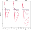 |
Fig. 3. Same as in Fig. 2, but for a Gaussian distributed force fluctuation field. |
| In the text | |
|
Fig. 4. Time evolution of the log radial position of the zone of avoidance for a population of BSS with masses mBSS = 1.5m* (empty circles) and mBSS = 2m* (filled circles), initially placed on randomly chosen isotropically distributed orbits. Time is measured in units of 104 dynamical crossing times. The orange circles refer to models employing a Holtsmark distribution of force fluctuations, while the blue circles refer to models where a three-dimensional Gaussian distribution of fluctuations was used. Plotted to guide the eye are a local polynomial regression (solid lines) fitted to the mBSS = 2m* zone of avoidance position for Holtsmark (orange) and Gaussian (blue) force kicks. Isotropic orbits are often assumed in most simple models of star clusters (e.g. King, Plummer); the results still hold even in the two extreme anisotropic scenarios where all orbits are circular (see Fig. 5) or radial (see Fig. 6). |
| In the text | |
|
Fig. 5. Time evolution of the log radial position of the zone of avoidance for a population of BSS with masses mBSS = 1.5m* (empty circles) and mBSS = 2m* (filled circles), initially placed on purely circular orbits. Time is measured in units of 104 dynamical crossing times. The orange circles refer to models employing a Holtsmark distribution of force fluctuations, while the blue circles refer to models where a three-dimensional Gaussian distribution of fluctuations was used. Plotted to guide the eye are a local polynomial regression (solid lines) fitted to the mBSS = 2m* zone of avoidance position for Holtsmark (orange) and Gaussian (blue) force kicks. Circular and radial orbits (see Fig. 6) are two extreme cases considered to show that the results are robust to changes in the distribution of BSS orbital angular momenta. |
| In the text | |
|
Fig. 6. Time evolution of the log radial position of the zone of avoidance for a population of BSS with masses mBSS = 1.5m* (empty circles) and mBSS = 2m* (filled circles), initially placed on purely radial orbits. Time is measured in units of 104 dynamical crossing times. The orange circles refer to models employing a Holtsmark distribution of force fluctuations, while the blue circles refer to models where a three-dimensional Gaussian distribution of fluctuations was used. Plotted to guide the eye are a local polynomial regression (solid lines) fitted to the mBSS = 2m* zone of avoidance position for Holtsmark (orange) and Gaussian (blue) force kicks. Radial and circular orbits (see Fig. 5) are two extreme cases considered to show that the results are robust to changes in the distribution of BSS orbital angular momenta. |
| In the text | |
Current usage metrics show cumulative count of Article Views (full-text article views including HTML views, PDF and ePub downloads, according to the available data) and Abstracts Views on Vision4Press platform.
Data correspond to usage on the plateform after 2015. The current usage metrics is available 48-96 hours after online publication and is updated daily on week days.
Initial download of the metrics may take a while.