| Issue |
A&A
Volume 639, July 2020
|
|
|---|---|---|
| Article Number | L7 | |
| Number of page(s) | 5 | |
| Section | Letters to the Editor | |
| DOI | https://doi.org/10.1051/0004-6361/202038576 | |
| Published online | 13 July 2020 | |
Letter to the Editor
Prospects for radio detection of stellar plasma beams
1
ASTRON, Netherlands Institute for Radio Astronomy, Oude Hoogeveensedijk 4, 7991 PD Dwingeloo, The Netherlands
e-mail: This email address is being protected from spambots. You need JavaScript enabled to view it.
2
Kapteyn Astronomical Institute, University of Groningen, Groningen, The Netherlands
Received:
3
June
2020
Accepted:
21
June
2020
Abstract
Violent solar eruptions are often accompanied by relativistic beams of charged particles. In the solar context they are referred to as solar particle events and are known to generate a characteristic swept-frequency radio burst. Due to their ionising potential, these beams influence atmospheric chemistry and habitability. Radio observations provide a crucial discriminant between stellar flares that do and do not generate particle beams. Here I use solar empirical data and semi-quantitative theoretical estimates to gauge the feasibility of detecting the associated radio bursts. My principal conclusion is that a dedicated search for swept frequency radio bursts on second timescales in existing low-frequency (ν ≲ 102 MHz) datasets, while technically challenging, will likely provide the evidence high-energy particles beams in Sun-like stars.
Key words: stars: coronae / radiation mechanisms: non-thermal / radio continuum: stars / plasmas
© ESO 2020
1. Introduction
Stellar activity can have a detrimental effect on the habitability of exoplanets. Violent releases of energy in the chromosphere and corona emit ionising radiation and eject plasma at high speeds into the interplanetary medium. The characteristic bolometric energy release in typical solar flare is about 1029 − 1032 ergs on timescales of minutes to hours (Emslie et al. 2012). Although this is comparable to or smaller than the bolometric output of the quiescent solar disc1, unlike quiescent solar emission, a large fraction of the flare energy goes into three components that are detrimental to the habitability: (a) ionising UV and X-ray radiation, (b) ejection of a large mass of coronal plasma at high speeds (CMEs), and (c) acceleration of charges to near-light speeds, the so-called solar particle events (SPEs).
Ever since the discovery of solar radio bursts, it was suspected that the radio emission is related to violent energy releases on the Sun (Payne-Scott 1949; Wild & McCready 1950). It is now well established that certain types of solar radio bursts are telltale signatures of SPE events (Winter & Ledbetter 2015; Miteva et al. 2017). In this paper I concentrate on SPEs and the unique value of radio observations in evidencing their nature on stars other than the Sun.
Solar particle events from solar flares usually carry about 5% of the total flare energy (Emslie et al. 2012). The particles range from keV level suprathermal energies to GeV scale relativistic energies (Schwenn 2006). Broadly speaking, the beam particles can be accelerated in two ways: magnetic reconnection in the chromosphere and lower corona leading to ‘impulsive’ events on timescales of seconds to minutes, and Fermi acceleration in a shock front2 leading to ‘gradual’ events on timescales of several minutes to an hour (Schwenn 2006; Desai & Giacalone 2016; Cairns et al. 2003).
A beam of high-energy particles moving in a dense thermal plasma leads to radio emission at the fundamental plasma frequency and its second harmonic (Benz 2002; Zheleznyakov 1996, and references therein). The characteristic radio bursts typically associated with impulsive and gradual particle beams are called type III and type II bursts, respectively (Ameri et al. 2019). The unique diagnostic value of radio bursts of type II and type III lies in the fact that the ambient plasma frequency must monotonically decrease as the particle beam moves radially outward from the flare site on an unbound trajectory. Plasma emission from such beams therefore sweeps down in frequency as a function of time providing clear evidence that the flare-accelerated particles will enter interplanetary space and influence the space weather around exoplanets.
These radio bursts from the Sun have been extensively studied both observationally and theoretically (Saint-Hilaire et al. 2013; Nita et al. 2002; Melrose 1980; Reid & Ratcliffe 2014). Analogous radio bursts have not been detected from other Sun-like stars, primarily due to sensitivity and time-on-sky limitations of previous searches. Furthermore, with few notable exceptions (see e.g. Bastian et al. 2018), previous searches have almost exclusively focused on highly active M dwarfs (Villadsen & Hallinan 2019; Osten & Bastian 2006; Crosley & Osten 2018a,b; Lynch et al. 2017) whose large-scale magnetic fields are about three orders of magnitude larger than the solar value. It is unclear if these stars emit interplanetary plasma beams or mass ejections at all (see below). In addition, the primary mechanism for bursts on these stars (and the underlying plasma instability) may be cyclotron emission due to their large magnetic field. In this case the emission likely traces high-energy plasma in magnetic traps rather than unbound plasma that streams into interplanetary space and influences space-weather around exoplanets. Consequently, the flare dynamics and phenomenology of the radio emission is likely to be fundamentally different from those on Sun-like stars with weak magnetic fields.
I must at the outset qualify what ‘Sun-like’ means in this context. Stellar flares have been routinely detected in optical (Yang & Liu 2019; Günther et al. 2020) and X-ray observations (Pye et al. 2015). These observations provide a reasonable estimate of the flare energy and duration, but do not provide a concrete picture of the dynamics of the flare. For example, although dMe stars are prone to extremely energetic flares that are many orders of magnitude brighter than typical solar flares, they also have large-scale magnetic fields that are orders of magnitude stronger than the solar value. It is therefore entirely plausible that despite the copious amounts of energy released, any plasma heated and/or accelerated in the flare is unable to force open the magnetic field lines and to unbind itself from the star. Therefore, I define Sun-like to mean stars of spectral class F, G, and K whose magnetic field structure and plasma dynamics during flares are most likely to be similar to the Sun. It is vital to note a crucial caveat, however. Recent studies have shown that the Sun is at a critical transition point in the nature of its magnetic activity (Metcalfe et al. 2016; van Saders et al. 2016). As such, extrapolating our accrued empirical knowledge on solar radio bursts to other Sun-like stars may be fraught. An explicit aim of searching for solar-type bursts on other stars is also to understand the evolution of solar activity over its lifetime by comparing it to an ensemble of stars of varying age.
If we hold the total radio energy constant, then a radio telescope is more sensitive to a shorter duration emission. It is therefore a prudent observational strategy to first go after type III radio bursts from impulsive beams. The same techniques can be brought to bear on the more gradual Type II events that are associated with coronal mass ejections. Thus motivated, the rest of this paper makes judicious predictions for the feasibility of detecting type III bursts from Sun-like stars in our Galactic neighbourhood.
2. Sun as a prototypical star
The simplest yield-estimate one can make is to assert that all target stars flare like the Sun. Saint-Hilaire et al. (2013) have collated flux-densities, source sizes, and brightness temperatures of isolated solar type III bursts from a decade of solar observations. They present data at different channels ranging from 150 to 430 MHz. Here I consider their statistics at 150 MHz. The numbers of bursts that exceed a flux density threshold of S is (Fig. 12 from Saint-Hilaire et al. 2013)
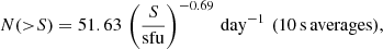 (1)
(1)
where 1 sfu = 104 Jy = 10−19 ergs cm−2. The empirical relationship was based on a sample of bursts, the brightest of which reached about ∼1010 Jy. It is important to note that these statistics are based on observations with 10 s exposures. The characteristic duration of type III bursts at 150 MHz is ∼1 s (Raoult & Pick 1980). Therefore, the measured flux densities of the singular bright bursts at the optimal exposure are likely to be ten times higher3. If the same ensemble of bursts were viewed from a distance of dpc parsec, then the number counts would be
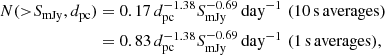 (2)
(2)
where SmJy is the observed flux density in mJy units.
It is interesting to first check whether the same distributions of bursts can be detected from nearby stars using the LOFAR telescope (van Haarlem et al. 2013). The LOFAR telescope has a zenith system equivalent flux density of about 47 Jy around 150 MHz. Solar type III bursts are known to have a duration of ∼1 s at 150 MHz (Raoult & Pick 1980) and a spectral drift rate of ≈100 MHz s−1 (Alvarez & Haddock 1973). For purposes of sensitivity calculations at 150 MHz, we can simply assume the burst to be a wide-band source over an instantaneous bandwidth of 40 MHz that is typical for LOFAR observations. The 5σ detection limit4 for a 40 MHz bandwidth and 1 s exposure is Slofar ≈ 25 mJy and ≈8 mJy in a 10 s exposure.
One can get an intuition for LOFAR’s sensitivity by noting that the type III bursts of the closest G dwarf, Alpha Centauri can be detected at a rate of one type III burst every 16 days of on-sky time. It is also noteworthy that the 25 mJy threshold corresponds to a burst that would be 109 Jy if viewed from 1 AU, and bursts of such brightness are detected by regular solar monitoring programmes (Saint-Hilaire et al. 2013; Nita et al. 2002). In other words, the first extra-solar type III burst is a ‘guaranteed’ discovery with state-of-the-art radio instrumentation5. Moving further out, Epsilon Eridani is a K dwarf at a distance of 3.2 pc that must be observed, on average, for about 50 days to score a detection. Here still the detectable bursts will be about 1010 Jy when viewed from 1 AU which is still within the bright end of observed solar bursts. Regardless, the wait time is likely to be overly conservative because Epsilon Eridani, owing to its youth, is more active than the middle-aged Sun.
Moving further out, our adopted value of 1011 Jy for the brightest solar burst will be detectable from stars out to dpc ≈ 10. There are about 100 G dwarfs and 300 K dwarfs in this volume (Henry et al. 2018). Even if they all flared in the same way as the Sun, then the observed flare counts from a volume out to  based on Eq. (1) is
 (3)
(3)
For the LOFAR case, with a 25 mJy detection threshold, the all-sky rate of solar brightness bursts is N ≈ 0.06 day−1 (4π sr)−1.
To gauge detectability at distances exceeding 10 pc, we invariably have to extrapolate beyond the observed solar brightness range.
3. Ensemble of flaring stars
The solar flare energy distribution spans many orders of magnitude. The brightest solar flares have a bolometric output of ∼1032 ergs. Observations of Sun-like stars have shown that about ∼1% of stars display super-flares with a bolometric output of 1032 − 1036 ergs (Yang & Liu 2019; Günther et al. 2020). It is reasonable to expect that the accompanying radio emissions will be significantly brighter because both the radio and optical emission are ultimately powered by the same engine. Here I adopt the simplest extrapolation in brightness possible: the radio brightness scales in proportion to the optically inferred flare energy.
Although such an extrapolation is admittedly simplistic, it is comforting to note the rough parity between the rates of solar radio bursts and solar flares. A consensus view from several solar flare observations is that the flare energy follows a power-law distribution with slope of ≈ − 1 (integral counts) and a normalisation that corresponds to about one bright flare of ∼1032 ergs every 102 days (Schrijver et al. 2012, their Fig. 3). If we assume that all burst are 1 s long, then their true flux densities will be ten times greater than those reported by Saint-Hilaire et al. (2013) using 10 s exposures (Eq. (1)). Then, the brightest type III bursts will have a flux density of 1011 Jy and occur at a rate of 0.004 day−1. Therefore, I assert the following relationship to extrapolate the radio fluxes to more energetic super-flares:
 (4)
(4)
Armed with this relationship, we can readily predict the radio flux distribution from an ensemble of Sun-like stars. Let the volume density of the target stars be ρ in units of per cubic parsecs, and their flare energies distributed according to N(> E) = C32(E/1032 ergs)α in units of day−1 star−1. The time rate of arrival of radio bursts brighter than some threshold from all stars within a distance  is then
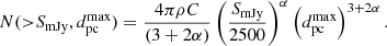 (5)
(5)
The constants C32 and α for a large population of stars of various spectral types have been well constrained by the Kepler emission, particularly for large flares in the range 1032 − 1036 ergs. Here I adopt the rates published by Yang & Liu (2019). Only 1.46% of the targeted G dwarfs show detectable flaring activity. For this flaring sample, C32 = 4.8 and α = −0.966. There are 0.0045 G dwarfs per cubic parsec in the solar neighbourhood (Henry et al. 2018), which means the volumetric rate of G dwarfs with detected super-flares is ρ = 6.6 × 10⁻⁵ pc−3. Substituting these values in Eq. (5), we get
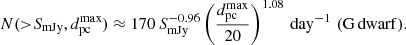 (6)
(6)
Similarly, for K dwarfs we have, 0.01 stars per cubic parsec (Henry et al. 2018) and 2.96% are known to display super-flares with C32 = 0.55, α = −0.78 (Yang & Liu 2019). This gives ρ = 3 × 10⁻⁴ pc−3 and
 (7)
(7)
The values diverge as  because the flare counts are sufficiently flat and we have not applied an upper bound on the brightness of radio emission. We address this next.
4. Peak brightness of bursts
Regardless of the flare energy, the peak brightness of bursts will be ultimately limited by the physics of the radiation mechanism. The mechanism of plasma emission from a particle beam is a two-stage process. Plasma density oscillations called Langmuir waves are first emitted by the beam particles. The Langmuir waves then scatter on ambient thermal ions or ion sound waves and are converted to electromagnetic waves that can escape the source (see Benz 2002; Zheleznyakov 1996; Melrose 1980; Kaplan & Tsytovich 1973 for further details).
Both stages have limits on the intensity of waves that can be sustained. First, the energy density of Langmuir waves is thought to be limited to about w ∼ 10−5 of the background thermal energy density NkBT, where N is the thermal plasma density, T is the temperature and kB is Boltzmann’s constant (Benz 2002). Beyond w ∼ 10−5, the Langmuir waves begin to alter the dispersion relationship in the background plasma leading to a runaway refraction and collapse of wave packets. In the second stage the brightness temperature to which the electromagnetic waves can grow, Tb, is limited to that of the Langmuir waves, TL. In the contrary situation the reverse process (electromagnetic to Langmuir) would become dominant and bring about equilibrium between the two species of radiation (Melrose 1980; Kaplan & Tsytovich 1973).
Consider a beam of particles with a small velocity spread Δvb around vb. Langmuir waves around a wavenumber, kL = ωp/vb, and a spread, ΔkL/kL = Δvb/vb, will then be in resonance with the beam particles. Here ωp is the angular plasma frequency and we have used the fact that Langmuir waves only exist in a small frequency range around ωp. Let the beam have an opening angle of θb. The total wavenumber volume occupied by the Langmuir waves is  . Since the energy density of Langmuir waves is wNkBT, their Rayleigh-Jeans temperature is
 (8)
(8)
which at 150 MHz for a saturation value of w = 10−5, beam velocity of vb = 0.3c, and a typical solar coronal value of T = 2 × 10⁶ K is
 (9)
(9)
Precise values of the velocity spread and the beam opening angle are not directly accessible even in the solar corona. As such, their normalisation points in Eq. (9) are educated guesses and the brightness temperature must be taken as a rough order-of-magnitude estimate. It is also important to note that the value of  in Eq. (9) agrees with that estimated with more detailed semi-quantitative estimates of Melrose (1980). They explicitly considered the growth rate of Langmuir waves due to the beam instability to be balanced by diffusion of the waves in angle (and hence out of resonance with the beam) due to density inhomogeneities on scales larger than the waves themselves. I have instead absorbed that balance into the parameter w ∼ 10−5, which is also based on diffusion of Langmuir waves in angle due to density inhomogeneities.
Having determined the peak brightness temperature of type III radiation, we are faced with a fresh problem. Because only flux density can be measured, we need to know the size of the emitter in order to make use of the brightness temperature. It is tempting to relate the transverse size of the emitter to the opening angle of the particle beam. This is however fraught in the case of emission at the fundamental because of the heightened level of wave refraction and scattering close to the plasma frequency (Melrose 1980). Such propagation effects are indeed to blame for the low observed polarised fraction of solar type III bursts even though the emission mechanism itself predicts 100% o-mode polarisation. A pragmatic way forward is to assign the measured median source size of 5′ (FWHM at 1 AU) measured for solar bursts at 150 MHz (Saint-Hilaire et al. 2013) and assume a constant solid-angle broadening factor of 102 as inferred for solar bursts (Melrose 1980).
The peak flux density of a source operating close to saturation at a distance of dpc parsec is then readily found to be7
 (10)
(10)
In other words, given the sensitivity of existing telescopes like LOFAR at 150 MHz, the distance-horizon for super-flares is ∼100 pc.
We can now also bound the flux density in our simple model of Eq. (4) to relate super-flare energy to radio burst flux density. The peak radio spectral luminosity at saturation (from Eq. (10)) is ∼350 Jy pc2, or about 1016.5 erg s−1 Hz−1. Putting this in Eq. (4), I find that the radio luminosity from metre-wave radio bursts saturates at a bolometric flare energy of ∼1034 erg. Saturation, therefore, leads us to modify Eq. (4):
 (11)
(11)
Equations (6) and (7) remain valid so long as  and SmJy are chosen to obey Eq. (10). In summary, the emission mechanism combined with empirical constraints on apparent source size show that, to account for super-flare related emission, it is reasonable to scale the radio flux densities up to a factor of ∼102 from the brightest solar bursts ever observed.
5. Outlook
The arguments presented here lead to a two-fold observational strategy for the discovery of extrasolar type III bursts. First, as the flare statistics of more nearby stars (dpc ∼ 10) become available with TESS data, one can use the estimates presented here to identify promising Sun-like stars for targeted campaigns to go after ∼1032 − 33 erg flares. These are normal flares for which empirical solar radio data can be applied in a comparative study. Second, the ensemble flare statistics for super-flares (E ≫ 1032 ergs) are already constrained by Kepler data. The larger horizon distances for super-flares allows searches in existing archival data. For example, the ongoing LoTSS survey with LOFAR (Shimwell et al. 2019) is surveying the northern sky at 150 MHz using 3168 pointings, each lasting 8 h8. The instantaneous FWHM field of view of LOFAR is about 16 deg2. This amounts to ∼105.5 deg2 h of sky exposure. Assuming a 10σ detection threshold of 50 mJy, we get a distance horizon of 85 pc, which yields an all-sky rate from Eqs. (6) and (7) of ≈101.6 day−1 (4π sr)−1 (see also Fig. 1). The bursts will originate from N* ≈ 103 stars capable of super-flares, which means each LOFAR pointing will have about 0.4 such stars on average. The total yield over the planned 3168 8 h survey pointings is therefore ≳101 events which is very promising, but not absolutely guaranteed, due to the inherent uncertainties involved.
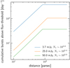 |
Fig. 1. Expected all-sky rate of radio bursts at 150 MHz accompanying super-flares (E ≫ 1032 erg) from stars within a distance given by the x-axis values. The different curves correspond to the flux-sensitivity thresholds given in the legend. The thresholds correspond to the planned SKA-low sensitivity (blue), and current LOFAR sensitivity (optimistic in orange and conservative in green) in a 1 s integration and 40 MHz bandwidth, respectively. The break in the curves is at the sensitivity horizon, and is due to saturation of the emission process. The expected number of stars within the horizon contributing to the super-flares is also given in the legend. |
I end by noting two caveats. First, the estimates related to super-flares presented here must be taken as being order of magnitude values as they are based on semi-quantitative arguments. Although inherent uncertainty will remain until real detections are brought to bear, modelling of expected burst spectra for different coronal parameters is a fruitful avenue for future work. Solar type III bursts attain peak brightness temperature at decametre wavelengths that are emitted at ∼10 R⊙. For instance, the brightest type III bursts are observed to have a flux density of 1012 Jy at 1 MHz (Dulk 2000), which is an order of magnitude higher than the peak 150 MHz flux density adopted here. The base coronal density values of stars prone to super-flares are likely much higher, and although it is tempting to postulate that their peak brightness will be attained at metre-wavelengths, further theoretical work is necessary to make an informed statement. Second, having achieved a detection, one is still faced with the task of demonstrating the swept frequency nature of the bursts, a necessary step to confirm the propagation of a plasma beam along an unbound trajectory. This may prove challenging in some cases where the observation bandwidth and time resolution do not allow for the frequency sweep to be unambiguously detected. Based on the solar experience, in such cases, type III bursts and the so-called spike bursts may be difficult to tell apart. Spike burst are thought to be driven by a different emission mechanism: the electron cyclotron maser, which can also attain very high brightness temperatures (Cliver et al. 2011). However, they occur on much shorter timescales (milliseconds to tens of milliseconds) and can therefore be readily distinguished from type III burst in data with sufficient resolution.
Hence we cannot see solar flares with our eyes.
Shock formation requires bulk ejection of thermal coronal plasma at super-Alfvénic speeds and does not happen in all flares.
Type III ‘storms’ with a train of bursts do occur, but storm-related bursts are typically faint (Reid & Ratcliffe 2014).
For Gaussian statistics, 5σ corresponds to one false positive (noise spike) in ∼103 h of observation with 1 s exposures.
Unfortunately Alpha Centauri cannot be observed from LOFAR’s latitude.
I estimate C32 and α using the data point at 1035 ergs in their Fig. 15 and power-law indices from their Fig. 3.
One can check that the adopted peak flux density for solar bursts of 1011 Jy gives Tb ≲ 1015 K, which is comfortably within the theoretical maximum for scatter broadening of the solid angle by factors of up to 103.
The survey data are archived at the necessary 1 s resolution.
Acknowledgments
I thank Prof. Gregg Hallinan for introducing me to the subject of extra-solar space weather, and Dr. Hamish Reid for a short albeit interesting discussion on this topic. I thank Dr. Ben Pope and Dr. Joe Callingham for commenting on the manuscript and the anonymous referee for helpful comments.
References
- Alvarez, H., & Haddock, F. T. 1973, Sol. Phys., 29, 197 [NASA ADS] [CrossRef] [Google Scholar]
- Ameri, D., Valtonen, E., & Pohjolainen, S. 2019, Sol. Phys., 294, 122 [CrossRef] [Google Scholar]
- Bastian, T. S., Villadsen, J., Maps, A., Hallinan, G., & Beasley, A. J. 2018, ApJ, 857, 133 [CrossRef] [Google Scholar]
- Benz, A. 2002, Plasma Astrophysics, Second Edition (Dordrecht: Kluwer Academic Publishers), 279 [Google Scholar]
- Cairns, I. H., Knock, S. A., Robinson, P. A., & Kuncic, Z. 2003, Space Sci. Rev., 107, 27 [NASA ADS] [CrossRef] [Google Scholar]
- Cliver, E. W., White, S. M., & Balasubramaniam, K. S. 2011, ApJ, 743, 145 [CrossRef] [Google Scholar]
- Crosley, M. K., & Osten, R. A. 2018a, ApJ, 862, 113 [CrossRef] [Google Scholar]
- Crosley, M. K., & Osten, R. A. 2018b, ApJ, 856, 39 [NASA ADS] [CrossRef] [Google Scholar]
- Desai, M., & Giacalone, J. 2016, Liv. Rev. Sol. Phys., 13, 3 [Google Scholar]
- Dulk, G. A. 2000, Washington DC American Geophysical Union Geophysical Monograph Series, 119, 115 [Google Scholar]
- Emslie, A. G., Dennis, B. R., Shih, A. Y., et al. 2012, ApJ, 759, 71 [NASA ADS] [CrossRef] [Google Scholar]
- Günther, M. N., Zhan, Z., Seager, S., et al. 2020, AJ, 159, 60 [CrossRef] [Google Scholar]
- Henry, T. J., Jao, W.-C., Winters, J. G., et al. 2018, AJ, 155, 265 [NASA ADS] [CrossRef] [Google Scholar]
- Kaplan, S. A., & Tsytovich, V. N. 1973, in Plasma Astrophysics (Oxford: Pergamon Press), Int. Ser. Monogr. Nat. Philos. [Google Scholar]
- Lynch, C. R., Lenc, E., Kaplan, D. L., Murphy, T., & Anderson, G. E. 2017, ApJ, 836, L30 [NASA ADS] [CrossRef] [Google Scholar]
- Melrose, D. B. 1980, Space Sci. Rev., 26, 3 [NASA ADS] [CrossRef] [Google Scholar]
- Metcalfe, T. S., Egeland, R., & van Saders, J. 2016, ApJ, 826, L2 [Google Scholar]
- Miteva, R., Samwel, S. W., & Krupar, V. 2017, J. Space Weather Space Clim., 7, A37 [CrossRef] [EDP Sciences] [Google Scholar]
- Nita, G. M., Gary, D. E., Lanzerotti, L. J., & Thomson, D. J. 2002, ApJ, 570, 423 [NASA ADS] [CrossRef] [Google Scholar]
- Osten, R. A., & Bastian, T. S. 2006, ApJ, 637, 1016 [NASA ADS] [CrossRef] [Google Scholar]
- Payne-Scott, R. 1949, Aust. J. Sci. Res. A Phys. Sci., 2, 214 [Google Scholar]
- Pye, J. P., Rosen, S., Fyfe, D., & Schröder, A. C. 2015, A&A, 581, A28 [NASA ADS] [CrossRef] [EDP Sciences] [Google Scholar]
- Raoult, A., & Pick, M. 1980, A&A, 87, 63 [NASA ADS] [Google Scholar]
- Reid, H. A. S., & Ratcliffe, H. 2014, Res. Astron. Astrophys., 14, 773 [NASA ADS] [CrossRef] [Google Scholar]
- Saint-Hilaire, P., Vilmer, N., & Kerdraon, A. 2013, ApJ, 762, 60 [NASA ADS] [CrossRef] [Google Scholar]
- Schrijver, C. J., Beer, J., Baltensperger, U., et al. 2012, J. Geophys. Res. (Space Phys.), 117, A08103 [Google Scholar]
- Schwenn, R. 2006, Liv. Rev. Sol. Phys., 3, 2 [Google Scholar]
- Shimwell, T. W., Tasse, C., Hardcastle, M. J., et al. 2019, A&A, 622, A1 [NASA ADS] [CrossRef] [EDP Sciences] [Google Scholar]
- van Haarlem, M. P., Wise, M. W., Gunst, A. W., et al. 2013, A&A, 556, A2 [NASA ADS] [CrossRef] [EDP Sciences] [Google Scholar]
- van Saders, J. L., Ceillier, T., Metcalfe, T. S., et al. 2016, Nature, 529, 181 [NASA ADS] [CrossRef] [PubMed] [Google Scholar]
- Villadsen, J., & Hallinan, G. 2019, ApJ, 871, 214 [NASA ADS] [CrossRef] [Google Scholar]
- Wild, J. P., & McCready, L. L. 1950, Aust. J. Sci. Res. A Phys. Sci., 3, 387 [Google Scholar]
- Winter, L. M., & Ledbetter, K. 2015, ApJ, 809, 105 [CrossRef] [Google Scholar]
- Yang, H., & Liu, J. 2019, ApJS, 241, 29 [CrossRef] [Google Scholar]
- Zheleznyakov, V. V. 1996, Radiation in Astrophysical Plasmas (Dodrecht: Kluwer Academic Publishers), 204 [CrossRef] [Google Scholar]
All Figures
|
Fig. 1. Expected all-sky rate of radio bursts at 150 MHz accompanying super-flares (E ≫ 1032 erg) from stars within a distance given by the x-axis values. The different curves correspond to the flux-sensitivity thresholds given in the legend. The thresholds correspond to the planned SKA-low sensitivity (blue), and current LOFAR sensitivity (optimistic in orange and conservative in green) in a 1 s integration and 40 MHz bandwidth, respectively. The break in the curves is at the sensitivity horizon, and is due to saturation of the emission process. The expected number of stars within the horizon contributing to the super-flares is also given in the legend. |
| In the text | |
Current usage metrics show cumulative count of Article Views (full-text article views including HTML views, PDF and ePub downloads, according to the available data) and Abstracts Views on Vision4Press platform.
Data correspond to usage on the plateform after 2015. The current usage metrics is available 48-96 hours after online publication and is updated daily on week days.
Initial download of the metrics may take a while.