| Issue |
A&A
Volume 638, June 2020
|
|
|---|---|---|
| Article Number | A153 | |
| Number of page(s) | 10 | |
| Section | Galactic structure, stellar clusters and populations | |
| DOI | https://doi.org/10.1051/0004-6361/202037764 | |
| Published online | 29 June 2020 | |
Populations of double white dwarfs in Milky Way satellites and their detectability with LISA
1
Institute for Gravitational Wave Astronomy, School of Physics and Astronomy, University of Birmingham, Birmingham B15 2TT, UK
e-mail: This email address is being protected from spambots. You need JavaScript enabled to view it.
; This email address is being protected from spambots. You need JavaScript enabled to view it.
2
Institute of Astronomy, Madingley Rd, Cambridge CB3 0HA, UK
3
Center for Cosmology and AstroParticle Physics, The Ohio State University, 191 West Woodruff Avenue, Columbus, OH 43210, USA
4
Leiden Observatory, Leiden University, PO Box 9513, 2300 RA Leiden, The Netherlands
Received:
18
February
2020
Accepted:
7
May
2020
Abstract
Context. Milky Way dwarf satellites are unique objects that encode the early structure formation and therefore represent a window into the high redshift Universe. So far, their study has been conducted using electromagnetic waves only. The future Laser Interferometer Space Antenna (LISA) has the potential to reveal Milky Way satellites through gravitational waves emitted by double white dwarf (DWD) binaries.
Aims. We investigate gravitational wave signals that will be detectable by LISA as a possible tool for the identification and characterisation of the Milky Way satellites.
Methods. We used the binary population synthesis technique to model the population of DWDs in dwarf satellites and we assessed the impact on the number of LISA detections when making changes to the total stellar mass, distance, star formation history, and metallicity of satellites. We calibrated predictions for the known Milky Way satellites on their observed properties.
Results. We find that DWDs emitting at frequencies ≳3 mHz can be detected in Milky Way satellites at large galactocentric distances. The number of these high frequency DWDs per satellite primarily depends on its mass, distance, age, and star formation history, and only mildly depends on the other assumptions regarding their evolution such as metallicity. We find that dwarf galaxies with M⋆ > 106 M⊙ can host detectable LISA sources; the number of detections scales linearly with the satellite’s mass. We forecast that out of the known satellites, Sagittarius, Fornax, Sculptor, and the Magellanic Clouds can be detected with LISA.
Conclusions. As an all-sky survey that does not suffer from contamination and dust extinction, LISA will provide observations of the Milky Way and dwarf satellites galaxies, which will be valuable for Galactic archaeology and near-field cosmology.
Key words: gravitational waves / binaries: close / white dwarfs / galaxies: dwarf / Local Group / Magellanic Clouds
© ESO 2020
1. Introduction
Dwarf galaxies are the first baryonic systems to appear in the Universe. The Λ cold dark matter (ΛCDM) cosmological model predicts that dwarf galaxies develop from small fast-growing lumps of dark matter that are able to accrete and cool down enough gas to form stars. State-of-the-art ΛCDM cosmological dark matter-only simulations predict the existence of a large number of small dark matter halos, which are large enough to host dwarf galaxies, within the Milky Way-like halos (e.g. Springel et al. 2008; Kuhlen et al. 2009; Stadel et al. 2009; Garrison-Kimmel et al. 2014). Over time, a fraction of these dwarf galaxies are destroyed by the gravitational pull of the Milky Way and now form the diffuse halo of our Galaxy (e.g. Bullock & Johnston 2005). Those that survived are known as Milky Way satellites. Both satellites and stars of the diffuse halo bear the Galactic archaeological record and are, therefore, precious tools to reconstruct the Milky Way formation history.
About 60 satellite galaxies orbiting within the virial radius of the Milky Way are known to date, with stellar masses reaching down to ∼300 M⊙ (e.g. Simon 2019). This census is known to be highly incomplete (e.g. Koposov et al. 2009; Newton et al. 2018). Modern surveys such as the Sloan Digital Sky Survey (SDSS, see e.g. Willman et al. 2005; Belokurov et al. 2007; Torrealba et al. 2016) and the Dark Energy Survey (DES, e.g. Koposov et al. 2015; Bechtol et al. 2015; Drlica-Wagner et al. 2015) do not cover the entirety of the sky and are subject to detectability limits that depend on both the surface brightness of and the distance to the satellites (see Koposov et al. 2008; Tollerud et al. 2008). Even the upcoming Rubin Observatory Legacy Survey of Space and Time (Ivezić et al. 2019) would only be able to find about half of the expected dwarfs galaxies (Jethwa et al. 2018; Newton et al. 2018).
In a companion paper by Roebber et al. (2020), we show that the Laser Interferometer Space Antenna (LISA) can detect ultra-short period (≲10 min) double white dwarfs (DWDs) that are hosted in Milky Way satellites, and that using the LISA data we can associate them to the host. Therefore, LISA will provide a complementary survey to study the satellites. In this paper we investigate the properties of DWD populations in satellites and how they are affected by, for example, star formation history (SFH) and metallicity (Z) of the satellites. Among the variety of stellar-mass binaries that will be observable by LISA, we focus on DWDs because they are expected to be the most numerous gravitational wave (GW) sources for a given galaxy mass (e.g. Nelemans et al. 2001a; Breivik et al. 2019).
The intrinsic faintness of white dwarf stars in the optical band limits their detection to distances of only a few kiloparsecs even for state-of-the-art facilities; the farthest known DWD is at 2.5 kpc (Burdge et al. 2019). Thus, no confirmed detections outside the Milky Way are known to date. The only exception is the X-ray source, RX J0439.8-6809, that has been tentatively identified as an accreting white dwarf in a compact binary system with a Helium white dwarf donor in the Large Magellanic Cloud (Greiner et al. 1994; van Teeseling et al. 1997). However, later spectral modelling suggests that this binary is also consistent with an unusually hot white dwarf in the Milky Way halo (Werner & Rauch 2015).
A number of theoretical studies predict that tens of thousands of Milky Way DWDs should be detectable by LISA (Nelemans et al. 2001b; Ruiter et al. 2010; Korol et al. 2017; Breivik et al. 2019; Lamberts et al. 2019); outside the Galaxy, DWDs can be detected out to the edge of the Local Group, and specifically up to a few tens of sources should be observed in the Andromeda galaxy (Korol et al. 2018). Although black hole and neutron star binaries are stronger GW emitters in the LISA band compared to DWDs, their rates are expected to be at least three orders of magnitude lower in the Milky Way and only a few sources are predicted to be detectable in nearby massive satellites (e.g. Andrews et al. 2019; Lau et al. 2020; Sesana et al. 2020; Seto 2019).
Leveraging large cosmological simulations, Lamberts et al. (2019) have shown that DWDs can indeed be detected by LISA in both satellites and tidal stellar streams. Crucially, the overall number of detections depends on the detailed properties of the considered halo and its accretion history. Cosmological simulations consider global solutions but the specific distribution of observed Milky Way satellites is not reproduced yet. In this paper we take a pragmatic approach to estimate the DWD population in Galactic satellites. We simulate individual DWD populations tuned on the properties of different satellites and investigate the expected number of LISA detections as a function of total stellar mass, distance, SFH, and metallicity of the satellites. By directly calibrating predictions on the observed properties of the known Milky Way satellites, our approach allows us to draw solid forecasts on the expected number of detections for the LISA mission. More importantly, we provide estimates for the range of expected detections and demonstrate how they depend on the main astrophysical processes at work. This allow us to make conclusions on additional and/or complementary information that LISA observations could offer for studying Milky Way satellites.
The outline of this manuscript is as follows. In Sect. 2 we describe our DWD population synthesis procedure as well as our dwarf-galaxy model. In Sect. 3 we report our results for a generic satellite and also present the number of predicted detections in the currently known Milky Way satellite population. In Sect. 4 we compare DWDs against electromagnetic (EM) mass-tracers and discuss how DWD observations with LISA can be used to measure the satellite properties. Finally, we summarise our results in Sect. 5.
2. Method
In this study we perform binary population synthesis to assess the prospects of GW detections in Milky Way dwarf satellites. Calculations are performed using the publicly available code SeBa (Portegies Zwart & Verbunt 1996; Toonen et al. 2012) that models the formation of DWDs starting from Zero-age Main-sequence (ZAMS) stars. Synthetic catalogues of DWDs produced with SeBa have been carefully calibrated against state-of-the-art observations of DWDs in terms of both mass ratio distribution (Toonen et al. 2012) and number density (Toonen et al. 2017). We construct different models at different metallicity, SFH, and treatment of the unstable mass-transfer phase (the so-called common envelope, CE). Each SeBa model consists of 3 × 10⁶ binaries at birth that roughly correspond to 107 M⊙ in total.
2.1. Initial binary population
We initialise the progenitor binary population as follows. Studies of Galactic globular clusters, the Magellanic Clouds (LMC, SMC), and local dwarf spheroidal galaxies find that the resolved stellar mass function appears to be consistent with that observed in the field populations and young forming clusters of the Milky Way (cf. Bastian et al. 2010). We adopt the Kroupa et al. (1993) initial mass function (IMF) for the mass of the primary star, m1. In this work, the primary (secondary) star is considered to be the initially most (least) massive star of the pair. We simulate primary stars in the mass range m1 ∈ [0.95 M⊙, 10 M⊙]. To calculate how many DWDs are present in a satellite of a given mass, we consider that stellar masses range from 0.1 to 100 M⊙. The mass of the secondary star m2 is drawn uniformly in [0.08 M⊙, m1] (Raghavan et al. 2010; Duchêne & Kraus 2013).
Semi-major axes a are drawn from a distribution that is uniform in log(a) (Abt 1983). We consider only detached binaries on the ZAMS with orbital separations up to 106 R⊙. Eccentricities e are initialised according to a thermal distribution in [0, 1] (Heggie 1975). Local dwarf galaxies show a diversity in metallicities ranging from roughly 0.0001 to Solar metallicity (see e.g. McConnachie 2012, and references therein). We adopt three different values: Z = 0.0001, 0.001, and 0.02, where the default is Z = 0.001. We set a constant binary fraction of 50%. This is appropriate for typical white dwarf progenitor (A- to F-type stars) at Solar metallicity, but it likely underestimates the multiplicity of early B-type stars (De Rosa et al. 2014; Duchêne & Kraus 2013; Moe & Di Stefano 2017).
2.2. Binary evolution
The progenitor of a DWD with orbital period P< a few hours typically undergoes two phases of mass transfer taking place when each of the stars evolves off the main sequence. Typically, at least one of these mass transfer phases is unstable and leads to a CE surrounding the binary (Paczynski et al. 1976; Webbink 1984). The CE evolution takes place on the timescale of thousand years, during which one of the two stars expands and engulfs the companion causing both objects to orbit inside a single, shared envelope (Ivanova et al. 2013). The companion star spirals inwards through the envelope, losing energy and angular momentum due to the dynamical friction. The temperature of the envelope consequently increases. This phase continues until the envelope is ejected from the system leaving behind the core of the expanded star and its companion in a tighter orbit.
We adopt two different treatments for the CE phase: the α-formalism based on the energy conservation and the γ-formalism based on the balance of angular momentum (for a review see Ivanova et al. 2013). More specifically, following Toonen et al. (2012) we make use of two evolutionary models, that we denote αα and γα. In model αα, the α-formalism is used to determine the outcome of every CE. For model γα the γ-prescription is applied unless the binary contains a compact object or the CE is triggered by a tidal instability, in which case α-prescription is used. For a typical evolution of a system according to the γα model, the first CE is typically described by the γ formalism, while the second by the α formalism. We highlight that the γα model is specifically calibrated for DWDs trough a reconstruction of the evolutionary paths of individual observed binaries (Nelemans et al. 2000, 2005; van der Sluys et al. 2006).
Our treatment of CE evolution has an effect on the DWD formation rate. In particular, model γα predicts about twice as many DWDs compared to model αα (Toonen et al. 2017). When restricting to those with orbital periods accessible to LISA, the two models are more similar. The predicted number of visible LISA sources in the Milky Way varies by ≲25% (Korol et al. 2017, see also Sect. 3 of this paper).
Figure 1 illustrates the synthetic population obtained by running SeBa with our fiducial assumptions and the CE γα-model. All binaries are initialised at the same time and evolved until both stars turn into white dwarfs. The x and y axes show orbital period P and chirp mass ℳ = (m1m2)3/5/(m1 + m2)1/5 of DWDs at birth, meaning that they do not encode any information about the type of the host galaxy. We describe how we transform these properties to account for the age and the SFH of the satellite galaxy in Sect. 2.3.1. The colour scale indicates their formation time measured from ZAMS. Dashed-dotted contours represent the binary merger time assuming that it is driven by GW radiation only (e.g. Maggiore 2008). Dashed lines delineate approximate boundaries between different core compositions of white dwarf components in our data (carbon-oxygen, CO; or helium, He). Figure 1 includes a number of features related to the choices made in binary population synthesis (for example a cutoff for DWDs with ℳ ≲ 0.4 M⊙ and P ≲ 10 min). These choices and their effects are fully detailed in Toonen et al. (2012).
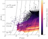 |
Fig. 1. Orbital periods P and chirp mass ℳ of DWDs at birth. The DWD formation time is represented by the colour scale, while their merger time by GW emission is represented by dashed-dotted contours (both timescales are expressed in Gyr). The figure shows only a fraction of the population with orbital periods accessible to LISA. Dashed lines represent approximate boundaries between DWDs of different types: CO+CO, CO+He and He+He; ONe white dwarfs represent a negligible fraction of the population and occupy the same part of the parameter space as CO+He ones. We also note that DWDs in this figure do not encode any information about the type of the host galaxy. |
DWDs tend to occupy the lower-right part of the parameter space and accumulate at long orbital periods and chirp masses of ∼0.5 M⊙. The formation time increases with decreasing chirp mass: in particular, at most a few Gyr are necessary to form more massive CO+CO and CO+He DWDs, while the formation of He+He systems takes several Gyr. The sum of the formation and merger times roughly indicates the lifespan of the binary. For instance, DWDs with formations times ≲1 Gyr (darker in Fig. 1) and merger timescales ≲10−3 Gyr (top-left in Fig. 1) are short-lived binaries and would generally inhabit star-forming environments. On the contrary, yellow circles in the bottom-right region of Fig. 1 require a longer time to form and merge, and would typically be present in old (≳10 Gyr) stellar populations. The age and SFH of the satellite play a crucial role in determining the properties of the resulting DWDs.
2.3. Synthetic satellites
Using the terminology of Bullock & Boylan-Kolchin (2017), systems with stellar mass M⋆ < 109 M⊙ are referred to as “dwarf” galaxies. Dwarfs are further subdivided into “bright” dwarfs (107 M⊙ < M⋆ < 109 M⊙), “classical” dwarfs with (105 M⊙ < M⋆ < 107 M⊙), and “ultra-faint” dwarfs (102 M⊙ < M⋆ < 105 M⊙). More specifically, we model satellites with masses M⋆ ∈ [103 M⊙ − 1010 M⊙], covering from ultra-faint dwarfs to Large Magellanic Cloud-analogues.
2.3.1. Star formation histories
The availability of detailed colour-magnitude diagrams for an increasing number of Local Group galaxies revealed that these systems have diverse SFHs, ranging from dwarfs dominated by old stars (≳12 Gyr ago) to nearly constantly star forming environments (Tolstoy et al. 2009; Brown et al. 2014; Weisz et al. 2014, 2019). It is generally found that the SFH depends on both the satellite’s mass and morphological type (spheroidal, elliptical, irregular, transitional). In particular, ultra-faint dwarf galaxies form 80% of their stellar mass by redshift z ∼ 2, while bright dwarfs produce only 30% of their stars by the same time (Weisz et al. 2014). This trend becomes more complicated if one considers the dwarf’s environment. Ultra-faint galaxies are generally found within the virial radius of the Milky Way, and thus experienced processes like tidal interactions and ram-pressure stripping that are known to quench star formation (e.g. Wetzel et al. 2015; Fillingham et al. 2018). In contrast, bright dwarfs are typically located outside the sphere of gravitational influence of the Milky Way, and are thus less likely to be influenced by the environment. Similar trends have been also observed in numerical simulations, such as APOSTLE (Sawala et al. 2016) and Auriga (Grand et al. 2017): galaxies with 105 < M⋆/M⊙ < 106 tend to have declining SFHs, massive dwarfs 107 < M⋆/M⊙ < 109 show an increasing star formation peaking at recent times, and the intermediate cases are found to form stars at a roughly constant rate (Digby et al. 2019).
To cover such a variety of cases we adopt three simple SFH models: single burst, constantly star-forming, and exponentially declining (also known as τ-model, Bruzual 1983). We adopt the exponentially declining model as our fiducial SFH model. For simplicity we assume that all satellites have the same age of 13.5 Gyr.
These different SFHs are implemented in our study as follows. For the single burst scenario, we model the DWD orbital evolution from their formation until 13.5 Gyr in which their orbits shrink through GW radiation reaction. We discard binaries if their formation times greater than 13.5 Gyr, they have begun mass transfer (i.e. when one of the white dwarfs fills its Roche lobe) or they have already merged within this time. These manipulations affect mostly short-lived systems and deplete the central part of Fig. 1. The constant SFH is produced by injecting DWD binaries into a satellite (accounting for the delay time between the parent binary and DWD formation, cf. Fig. 1) at the rate of 1 M⊙ yr−1 and subsequently evolving their orbits until present time. Over 13.5 Gyr, this model produces a galaxy of 13.5 × 10¹⁰ M⊙. The exponential SFH is constructed in a similar way, but the DWD injection rate decreases according to an exponential with characteristic timescale τ = 5 Gyr (Weisz et al. 2014). The result is then normalised to a total mass of 1010 M⊙. We note that more complex star formation scenarios can be constructed by combining the three basic ones described in this Section. In Fig. 2 we plot the cumulative distribution of the number of DWDs in the satellite galaxy for different star formation histories as a function of time.
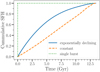 |
Fig. 2. Adopted SFHs: exponentially declining (blue solid), constant (orange dashed) and single burst 13.5 Gyr ago (green dotted). |
We evaluate the number of DWDs in a satellite galaxy of mass M⋆ by linearly re-scaling the simulation outputs
 (1)
(1)
where NDWD, SeBa is the number of DWDs in the synthetic population and where MSeBa is the total simulated population mass.
2.4. LISA detectability
LISA is an ESA-lead space mission designed to detect GW sources in the mHz frequency band (Amaro-Seoane et al. 2017). The diversity and large amount of GW signals simultaneously present in the LISA data stream make the data analysis extremely challenging (e.g. Babak et al. 2010; Littenberg et al. 2020). For simplicity, in this paper we use analytic prescriptions to assess the detectability of DWDs with LISA, allowing us to quickly process large populations. A companion paper by Roebber et al. (2020) carefully addresses prospects for detecting and characterising DWDs in Milky Way satellites with LISA.
For a typical DWD the timescale on which the orbital period changes due to the GW emission is significantly longer than the LISA mission lifetime, T. Therefore, one can safely approximate its signal as monochromatic with frequency f = 2/P. Averaging over sky location, polarisation, and inclination, one can write down the signal-to-noise ratio as (e.g. Robson et al. 2019):
 (2)
(2)
where 𝒜 is the amplitude of the signal
 (3)
(3)
Sn(f) is the power spectral density (PSD) of the detector noise in the low-frequency limit, G and c are respectively the gravitational constant and the speed of light, and R(f) is a transfer function encoding finite-armlength effects at high frequencies, tending to unity as f → 0. We compute R(f) numerically by averaging the full time-delay interferometry response of the detector to a monochromatic GW at each frequency as outlined in Larson et al. (2000). Approximate analytical expressions for R(f) are also given in Robson et al. (2019)1 and LISA Science Study Team (2018). Both agree well with our numerical result at frequencies below 20 mHz.
Current LISA specifications (LISA Science Study Team 2018) provide:
![Mathematical equation: $$ \begin{aligned}&S_{{n}}(f) = \frac{1}{L^2} \left[ \frac{4 S_{\rm {acc}}(f)}{(2 \pi f)^4} + S_{\rm {shot}}(f) \right], \end{aligned} $$](/articles/aa/full_html/2020/06/aa37764-20/aa37764-20-eq4.gif) (4)
(4)
![Mathematical equation: $$ \begin{aligned}&S_{\rm {acc}}(f)= \left( 3 \times 10^{-15} \mathrm{{~m}}/\mathrm{{s}}^2 \right)^2 \left[ 1 + \left(\frac{0.4 \mathrm{{~mHz}}}{f} \right)^2 \right] \mathrm{{Hz}}^{-1}, \end{aligned} $$](/articles/aa/full_html/2020/06/aa37764-20/aa37764-20-eq5.gif) (5)
(5)
 (6)
(6)
 (7)
(7)
We note that this PSD differs slightly from the one presented in the original LISA mission proposal (Amaro-Seoane et al. 2017, cf. Fig. 3). The two PSDs have a different frequency dependence at low frequencies, and are proportional to each other at high frequencies by a factor of 2/3. The updated curve penalises high frequency sources that, as we show later, are accessible at larger distances and therefore are optimal for detecting satellites. Both noise curves account for the confusion foreground noise produced by unresolved Galactic DWDs using the fitting expression of Babak et al. (2017).
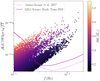 |
Fig. 3. Typical frequencies and characteristic strain for our fiducial population model (coloured circles) placed at d = 100 kpc. The colour scale shows the chirp mass distribution. Solid and dotted lines indicate the sky-, inclination and polarisation-averaged LISA sensitivity curve of LISA Science Study Team (2018) and that of Amaro-Seoane et al. (2017), respectively. |
We adopt the nominal (extended) mission duration time of 4 yr (10 yr). That is, we consider a formal duty cycle of 100% and ignore maintenance operations and data gaps due to, e.g. laser frequency switches, high-gain antenna re-pointing, orbit corrections, and unplanned events (e.g. Baghi et al. 2019). A more realistic assumption would be to consider a 70–80% duty cycle as achieved by the LISA Pathfinder mission (Armano et al. 2016), corresponding to ∼3 yr (∼8 yr) nominal (extended) mission duration. Using Eq. (2) one can re-scale the signal-to-noise ratio of any individual source (and thus the total number of detections by multiplying the nominal and extended mission results by  and
and  , respectively. A number of studies have assessed the detection threshold for monochromatic sources in the LISA data. For example, Crowder & Cornish (2007) report a detection threshold of ρthr = 5, while Błaut et al. (2010) a threshold of ρthr = 5.7. However, the former study did not include the frequency derivative in the search parameters, and neither one included the second derivative of the frequency or the orbital eccentricity, potentially important parameters to identify mass-transferring or triple systems (e.g. Nelemans et al. 2004; Robson et al. 2018; Tamanini & Danielski 2019). Including those extra parameters would tend to increase the detection threshold. Determining the new threshold would require a study beyond the scope of the present one, we therefore choose a somewhat conservative threshold of ρthr = 7. We verified that increasing the threshold to ρthr = 8 decreases the number of detected binaries by about 20%.
Figure 3 shows the sky-, inclination- and polarisation-averaged dimensionless characteristic strain of LISA,  (magenta solid line), and that of our fiducial population
  at d = 100 kpc (coloured circles). The fiducial DWD population was obtained starting from binaries represented in Fig. 1 and by computing their properties at the present time assuming that the satellite’s age is 13.5 Gyr and an exponentially declining SFH as described in Sect. 2.3.1.
In the parameter space represented in Fig. 3, the signal-to-noise ratio can be visually estimated as the height above the noise curve (e.g. Moore et al. 2015). For example, moving same population to d = 1 Mpc results into translating all circles down by a factor of 10. Because the distance is fixed, binaries occupy a narrow region in Fig. 3, which is set by the minimum and maximum chirp mass of the population (0.2 M⊙ ≲ ℳ ≲ 1.1 M⊙) as shown in colour.
3. Results
3.1. Effect of star formation history
Here we report the number of DWDs that can be detected by LISA in a given satellite galaxy with a stellar mass M⋆ at a distance d. Figure 4 presents results for our fiducial assumptions (Z = 0.001, Kroupa IMF, γα-CE evolution, and binary fraction of 50%) and the three different SFH models (exponentially declining, constant, and single burst). For all three SFH models we assume the age of the satellite to be 13.5 Gyr.
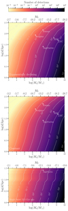 |
Fig. 4. Number of detectable DWDs in the log satellite mass – log distance parameter space for different SFH models: exponentially decreasing, constantly star-forming at the rate of 1 M⊙ yr−1 and single burst 13.5 Gyr ago. White stars represent known satellites listed in Table 2. The top x-axes shows the absolute magnitude in the V−band. The bottom panel is cut at log d∼1.6 as there are no more detectable sources at larger distances; this is the case of ultra-faint dwarfs, which have no sources detectable beyond this distance. |
Our exponential SFH model predicts a few million DWDs with orbital frequencies > 10−4 Hz. For a simulated total mass of 1010 M⊙ and assuming d = 100 kpc, we find ∼115 (∼294) detectable DWDs in the nominal (extended) LISA mission. The number of detections increases linearly with the satellite mass and decreases with its distance. This is shown in the top panel of Fig. 4. LISA sources are detectable in satellites with M⋆ ≳ 106 M⊙ (for instance the Sagittarius dwarf spheroidal galaxy, Ibata et al. 1994) up to ∼30 kpc, and in Magellanic Cloud-analogues with M⋆ ∼ 109 M⊙ up to 100 − 200 kpc (which corresponds to the virial radius of the Milky Way). We also find that our model predicts 3.4 × 10³ detections for M⋆ = 2 × 10¹⁰ M⊙ at d = 8.5 kpc. This is in agreement with estimates from Korol et al. (2019) for the MW bulge. In order to enable comparison with electromagnetic tracers, Fig. 4 shows the absolute V-band magnitude of the population, computed using the simple model of Bruzual & Charlot (2003) and the publicly available python package smpy.
The middle panel of Fig. 4 illustrates the number of detections for the constant SFH, keeping all other choices fixed to the fiducial model. In this case, satellites can be detected farther out in the Milky Way halo compared to those in the exponential SFH model. This is because a constant SFH produces a greater number of DWDs at recent times. We verify that the constant SFH model leads to 7 (51) detections for an Andromeda-like galaxy at the distance of 800 kpc for the nominal (extended) LISA mission lifetime, in agreement with earlier work of Korol et al. (2018).
Ultra-faint dwarfs typically stop forming stars after an initial burst (e.g. Weisz et al. 2014; Simon 2019). This scenario is represented in the bottom panel of Fig. 4. It is evident that ultra-faint dwarfs with M⋆ ≲ 105 M⊙ will be invisible to LISA. These satellites do not contain DWDs emitting at high frequencies, because they have already long since merged (cf. Fig. 1 for the relevant timescales). Only DWDs with frequencies f > 3 mHz can be detected and localised at distances ∼100 kpc as a consequence of the fact that (i) LISA is maximally sensitive around 3 − 5 mHz (see Fig. 3) and (ii) these frequencies are not affected by the confusion foreground (e.g. Littenberg & Cornish 2019).
Our results illustrate that the total stellar mass sets the fuel supply to generate DWDs, while the SFH together with the age of the satellite determine how many DWDs emit in the LISA frequency band at the present time. In particular, for a fixed satellite mass, age and distance the constant SFH produces on average twice as many detections compared to the exponential model, while the single burst produces only about half. Consequently, all three panels of Fig. 4 appear relatively similar when using a logarithmic scale. The crucial difference is given by the number of DWDs with f > 3 mHz hosted by a satellite at the present time. High frequency DWDs are more abundant in young and/or star-forming satellites. This is because the birthrate of DWDs peaks at early times (∼1 Gyr), and compact systems merge on shorter timescales (cf. Fig. 1). This is analogous to the case of massive DWD mergers studies in the context of type Ia-supernovae (e.g. Ruiter et al. 2007; Toonen et al. 2012; Claeys et al. 2014).
We summarise our results for the range of model variations in Table 1 using the example of a satellite with a total stellar mass of 2 × 10⁷ M⊙, an age of 13.5 Gyr, and a distance of 20 kpc.
Number of detectable DWDs in a satellite with total stellar mass of 2 × 10⁷ M⊙, age of 13.5 Gyr, and distance of 20 kpc for 4-year (10-year) long LISA mission assuming three SFH models: exponentially declining (fiducial), constantly star-forming and single burst.
3.2. Effect of metallicity
The number of detectable sources weakly increases with decreasing metallicity. For Solar metallicity the number of DWDs decreases by ∼20% compared to the default model (Z = 0.001) while at low metallicity (Z = 0.0001) the number of DWDs increases by ∼10% out to distances of 50 kpc (beyond this the number of sources is too low to establish any trend). Figure 5 shows that the number of detections depends only moderately on metallicity, with an overall variation in the predicted rates of less than a factor of 1.5 (see also Table 1). This is in stark contrast with the case of binary black holes mergers observable by LIGO where the metallicity impacts the formation rate by 1–3 orders of magnitude (e.g. Belczynski et al. 2010; Giacobbo et al. 2018; Neijssel et al. 2019). In general, metallicity alters the evolution of a star by changing its radius, core mass, and strength of the stellar winds. In case of the DWD evolution, metallicity mainly influences the minimum mass for an (isolated) star to reach the white dwarf stage in a Hubble time. This increases from 0.81 M⊙ at Z = 0.0001 to 0.82 M⊙ at Z = 0.001, and up to 0.98 M⊙ at Z = 0.02.
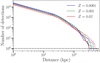 |
Fig. 5. Number of detections as a function of distance for a satellite of M⋆ = 1010 M⊙ with an exponentially decreasing SFH. Colours correspond to different values of metallicity: Z = 0.0001 in blue, Z = 0.001 in green and Z = 0.02 in red. Solid and dashed lines represent respectively γα- and αα-CE models. The dotted line shows the single-detection threshold. |
We are neglecting potential correlations between metallicity and primordial binary fraction. The advent of large and homogeneously selected samples indicates an anti-correlation for close (≲10 au) low-mass binaries (Badenes et al. 2018; El-Badry & Rix 2019; Moe et al. 2019, and references therein). For instance, Badenes et al. (2018) find that the multiplicity fraction of metal-poor stars (Z ≲ 0.005) is enhanced by a factor 2–3 compared to metal-rich stars (Z ≳ 0.02). Additionally, Spencer et al. (2018) found that the binary fraction is not constant across the Milky Way’s satellites. In particular, Draco and Ursa Minor presents binary fractions of 50% and 78% respectively. Enhancing the binary fraction from 50% to 70% (90%) in our simulations causes an increase of the number of detectable DWDs by a factor of ∼1.3 (1.6).
3.3. Source properties
Figure 6 illustrates the frequencies, chirp masses and ages (i.e. how long since the ZAMS) of detectable DWDs in our fiducial satellite of 1010 M⊙, 13.5 Gyr with the exponential SFH for a LISA mission of 4 yr. The blue line represents the overall population, whereas the green and red lines represent the populations detected respectively at 10 kpc (typical distances for stars in the Milky Way inner halo) and 100 kpc (typical distances for the outer halo). Sources with higher frequencies and higher chirp mass remain detectable with increasing distance. In particular, the median value of the frequency distribution shifts from ∼3 mHz at 10 kpc to ∼6 mHz at 100 kpc, while the median value of the chirp mass increases from 0.25 M⊙ to 0.5 M⊙ for the same values of d.
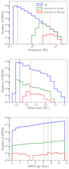 |
Fig. 6. Distribution of frequencies, chirp masses and ages of DWDs in our fiducial satellite model (blue), of those detected by LISA at 10 kpc (green) and 100 kpc (red). Vertical coloured lines mark medians of the respective distributions. |
In our fiducial model, the number of DWDs increases with increasing age (blue solid line in the bottom panel of Fig. 6) as a consequence of the adopted SFH and typical DWD formation timescales. The age distributions of binaries detected at 10 kpc (in green) does not show a strong selection effect compared to the overall population, although the median is shifted towards smaller ages. The selection effect is much stronger for the DWDs at 100 kpc (in red), shifting the median age to 8 Gyr. These are CO+CO and CO+He DWDs with higher chirp masses (see Fig. 1).
3.4. Known satellites
Ultra-faint dwarfs are unlikely to host detectable DWDs, therefore in this section we consider only classical and bright dwarfs with M⋆ ≥ 106 M⊙. We list stellar masses and distances of known satellites from McConnachie (2012) and report the number of LISA detections for our fiducial model in Table 2. Of all known satellites, only Sagittarius, Fornax, Sculptor, and the Magellanic Clouds host detectable LISA sources. For all the other satellites the probability of hosting LISA detections is ≲1%.
Number of detectable DWDs hosted in Milky Way satellites for nominal (4 yr) and extended (10 yr) mission duration derived using our fiducial exponentially declining SFH.
Dwarf galaxies show a large variation of SFHs even within the same class and morphological type (cf. Sect. 2.3.1). The SFH of the Sagittarius dwarf galaxy could be modelled by two events: a first one forming 50% of the total stellar mass > 12 Gyr ago, and the other forming the remaining 50% < 4 Gyr ago (Weisz et al. 2014). When adopting this more appropriate star formation scenario, the number of detections in Sagittarius increases to 10 DWDs for a 4 yr mission lifetime compared to 3 reported in Table 2. For the Fornax galaxy Weisz et al. (2014) reports a constant star formation history, that based on our binary population modelling predicts 0.2 detectable DWDs (cf. Fig. 4). On the other hand, Sculptor is perhaps better described by a single star formation event that occurred ∼12 Gyr ago, and thus our estimates are likely to be too optimistic for its case. Both Magellanic Clouds have recently (< 1 Gyr ago) experienced relevant star formation events (e.g. Strantzalis et al. 2019; Harris & Zaritsky 2009). Our declining star formation history models are likely to underestimate the number of detectable sources. For example, assuming a more optimistic constant SFH yields 100 (260) and 25 (55) detections respectively for the LMC and SMC assuming 4 (10) yr of LISA data. These brightest satellites will be targeted separately in a forthcoming paper by Keim et al. (in prep.).
In the companion paper by Roebber et al. (2020, Fig. 1) we show the distribution of the sky distribution of known satellites from Simon (2019), McConnachie (2012) highlighting those with detectable DWDs.
4. Discussion
Dwarf satellites with masses 106 − 109 M⊙ host DWDs radiating GWs at frequencies ≳3 mHz that are detectable by LISA out to distances of 10 − 300 kpc. Specifically, we find that ultra-faint dwarfs will not host DWDs because (i) their total stellar mass is too low and (ii) they form stars only at early times. Classical dwarfs can be detected at distances from a few to several tens of kiloparsecs only if they experienced a significant star formation at recent times. However, bright dwarfs with M⋆ > 108 M⊙ like the Magellanic Clouds can be detected at up to a few hundred kiloparsecs. Roebber et al. (2020) shows that these DWDs will not only be well localised on the sky (< 10 deg2 for ≥5 mHz), but their distances will be measured with precision of 10 − 40%. Shining bright in GWs, DWDs can be used as mass tracers at large galactocentric distances further enabling the characterisation of the Milky Way outer halo.
4.1. Comparison with electromagnetic mass tracers
Current EM mass tracers in the outer Milky Way typically represent collections of stars with a similar age, chemical composition and luminosity. Their 3D spatial distribution –sometimes also in combination with kinematics– is required to map the baryonic matter distribution in our Galaxy and in the entire Local Group. The most common and abundant stellar tracers present in optical surveys are main-sequence turn-off stars, blue horizontal branch stars, and M-giants stars (for a review see Belokurov 2013). These stellar classes are numerous, luminous, and can be selected with low levels of contamination.
Other commonly used mass tracers are variable stars such as RR Lyrae (RRL) and Cepheids. Variables have a well-determined relation between period and absolute luminosity and thus serve as standard candles to measure distances (e.g. Czerny et al. 2018). Interestingly, almost all dwarfs in the Local Group that have been studied so far contain at least one RRL (Baker & Willman 2015). This makes searches for stellar systems co-distant with RRLs a plausible mean to investigate sub-structures with low surface brightness (e.g. Sesar et al. 2014; Baker & Willman 2015; Torrealba et al. 2019).
In comparison, GW emitters such as DWDs do not present contaminants. Their GW signals can potentially be used to trace dwarf satellites all the way out to the virial radius of the Galaxy. Thus, DWDs are competitive with RRL stars that can be found up to ∼100 kpc in the Gaia data (Holl et al. 2018).
Newton et al. (2018) recently assessed the current observational limitations on the number of Milky Way dwarf satellites, and presented predictions for future optical surveys. Based on a number of cosmological simulations, they estimated that  dwarfs galaxies with MV ∼ 0 should be present within galactocentric distances of ≲300 kpc. Authors find that only half of predicted systems can be detected using the Rubin Observatory because of dust extinction and sky coverage limitations.
Although DWD observations do not suffer from any of these issues, they are much rarer compared to any of the aforementioned stellar mass tracers. The number of DWDs with f ≲ 3 mHz in a satellite is directly proportional to its total stellar mass, and quickly drops to zero for satellites with M⋆ < 106 M⊙ and no recent star formation. On the other hand, Roebber et al. (2020) show that DWDs with f ≳ 3 mHz will also have measurable frequency evolution, allowing distances to satellites to be measured.
4.2. Weighing the satellites with GWs
The number of LISA detections per satellite strongly depends on its total stellar mass (cf. Fig. 4). If a group of co-distant GW sources can be identified in the LISA data, one can then reverse-engineer our modelling process to get the mass of the (known or unknown) satellite. We stress that GW detections yield the original stellar mass of a satellite including the contribution of evolved stars that are no longer visible through light. This is in contrast to stellar masses derived from satellites’ EM brightness, sensitive to the mass enclosed in bright stars. Those kind of estimates are typically made by modelling the brightness of a satellite and applying age-dependent L/M ratios from stellar calculations which must necessarily adopt an IMF. This method is only sensitive to significant derivations from the nominal Kroupa-type IMF.
As an alternative, we use the IMF derived by Miller & Scalo (1979) which is flat below 1 M⊙ and is characterised by a higher mean mass of 0.65 M⊙ compared to 0.49 M⊙ for the Kroupa IMF. This IMF favours typical DWD progenitors. In comparison, the fiducial Kroupa IMF is more bottom-heavy and generates a higher number of low-mass stars that will need more than a Hubble time to turn into white dwarfs. We find that the Miller-Scalo IMF generates ∼10% more DWDs per 3 × 10⁷ M⊙, and, in particular, produces ∼30% more DWDs in the LISA band. This strong increase is largely due to the presence of more massive CO+CO DWDs. However when evolving the population to the age of the satellite (Sect. 2.3.1), these more massive short-lived CO+CO DWDs merge within a few Gyr, such that predominantly the low-frequency binaries (< 1 mHz) remain. As already discussed, these binaries are hardly detectable beyond ∼10 kpc. On the contrary, the Kroupa IMF generates more low-mass progenitors which take longer to turn into DWDs and evolve to mHz frequencies. Consequently, assuming a bottom-heavy IMF such as the Kroupa-IMF our simulations predicts more detections in satellites of intermediate and old age which are detectable at larger galactocentric distances.
As a quantitative example, we model the Sagittarius dwarf galaxy adopting a double-burst SFH and the age of 13.5 Gyr as described in Sect. 3.4. We find that the Miller-Scalo IMF predicts a similar number of LISA detections as the fiducial Kroupa IMF. However, DWDs in the former case with lower GW frequencies are difficult to identify as extra-galactic against the Galactic confusion foreground, due to large errors on the distance at low frequencies (Roebber et al. 2020). From this example we conclude that we can identify a relatively low-mass satellite in the Milky Way halo, provided its population originated from a more bottom-heavy IMF.
5. Conclusions
LISA can detect short-period DWDs beyond our galaxy, potentially reaching the outskirts of the Local Group. In this paper we assess what properties qualify a dwarf satellite galaxy as a host for LISA sources. We use a treatment tailored on individual Milky Way satellites. Complementary predictions where presented by Lamberts et al. (2019) using cosmological simulations. We use binary population synthesis to produce samples of DWDs for a putative galaxy with fixed binary fraction, metallicity, IMF, age and an analytic star formation model. Simulation results are then re-scaled to the mass of known Milky Way satellites. Our simple approach allows us to vary this set of assumptions and determine which region of the parameter space is optimal for hosting LISA sources. Specifically, our finding articulates as follows.
-
The number of DWDs strongly depends on the satellite’s total stellar mass. This limits LISA detections to satellites with M⋆ > 106 M⊙.
-
Both age and SFH influence the DWD orbital period distribution, and consequently number of binaries with f ≳ 3 mHz that are detectable at large distances. Because in young and star-forming satellites the birthrate of DWDs peaks at early times (∼1 Gyr), these systems are expected to host more DWDs emitting GWs in the LISA band.
-
Metallicity has a limited effect on DWD populations, with the total number of binaries increasing for decreasing metallicities.
-
Only DWDs with frequencies ≳3 mHz can be detected beyond the Milky Way stellar disc. This implies that all most of extra-galactic LISA detections will have measurable frequency derivative allowing to pin down the distance to the source with a relative error of ∼30% (Roebber et al. 2020). These DWDs can be used as mass tracers in the outer Milky Way much like Cepheids and RRL stars.
-
Of the known satellites only Sagittarius, Fornax, Sculptor and the Magellanic Clouds host detectable population of LISA sources.
-
If a suitable number of detections are identified within a satellite, inference on the satellite’s distance one can be used to estimate its total stellar mass.
As an all-sky survey that does not suffer from contamination and dust extinction, LISA can detect known Milky Way dwarf satellites and potentially discover new ones through populations invisible to EM instruments. Properties of these populations will inform us on the formation history of the Milky Way and its environs and provide unique contribution to Galactic archaeology and near-field cosmology.
We note that R(f) in Robson et al. (2019) is the inverse of our definition.
Acknowledgments
VK thanks J. Dalcantan for inspiring this study and K. Duncan for useful discussions on the observed electromagnetic properties of stellar populations. VK and ST acknowledge support from the Netherlands Research Council NWO (respectively Rubicon 019.183EN.015 and VENI 639.041.645 Grants). FV acknowledges support from the European Research Council Consolidator Grant funding scheme (project ASTEROCHRONOMETRY, G. A. No. 772293) and the support of a Fellowship from the Center for Cosmology and AstroParticle Physics at The Ohio State University. DG is supported by Leverhulme Trust Grant No. RPG-2019-350. AV acknowledges support from the Royal Society and the Wolfson Foundation. Computational work was performed on the University of Birmingham BlueBEAR cluster, the Athena cluster at HPC Midlands+ funded by EPSRC Grant No. EP/P020232/1, and the Maryland Advanced Research Computing Center (MARCC). This research made use of open source python package smpy, developed by K. Duncan and available at https://github.com/dunkenj/smpy, NumPy, SciPy, PyGaia python packages and matplotlib python library.
References
- Abt, H. A. 1983, ARA&A, 21, 343 [Google Scholar]
- Amaro-Seoane, P., Audley, H., Babak, S., et al. 2017, ArXiv e-prints [arXiv:1702.00786] [Google Scholar]
- Andrews, J. J., Breivik, K., & Chatterjee, S. 2019, ApJ, 886, 68 [NASA ADS] [CrossRef] [Google Scholar]
- Armano, M., Audley, H., Auger, G., et al. 2016, Phys. Rev. Lett., 116, 231101 [NASA ADS] [CrossRef] [Google Scholar]
- Babak, S., Baker, J. G., Benacquista, M. J., et al. 2010, Class. Quant. Grav., 27, 084009 [CrossRef] [Google Scholar]
- Babak, S., Gair, J., Sesana, A., et al. 2017, Phys. Rev. D, 95, 103012 [NASA ADS] [CrossRef] [Google Scholar]
- Badenes, C., Mazzola, C., Thompson, T. A., et al. 2018, ApJ, 854, 147 [NASA ADS] [CrossRef] [Google Scholar]
- Baghi, Q., Thorpe, I., Slutsky, J., et al. 2019, Phys. Rev. D, 100, 022003 [CrossRef] [Google Scholar]
- Baker, M., & Willman, B. 2015, AJ, 150, 160 [CrossRef] [Google Scholar]
- Bastian, N., Covey, K. R., & Meyer, M. R. 2010, ARA&A, 48, 339 [NASA ADS] [CrossRef] [Google Scholar]
- Bechtol, K., Drlica-Wagner, A., Balbinot, E., et al. 2015, ApJ, 807, 50 [NASA ADS] [CrossRef] [Google Scholar]
- Belczynski, K., Dominik, M., Bulik, T., et al. 2010, ApJ, 715, L138 [NASA ADS] [CrossRef] [Google Scholar]
- Belokurov, V. 2013, New Astron. Rev., 57, 100 [NASA ADS] [CrossRef] [Google Scholar]
- Belokurov, V., Zucker, D. B., Evans, N. W., et al. 2007, ApJ, 654, 897 [NASA ADS] [CrossRef] [Google Scholar]
- Błaut, A., Babak, S., & Królak, A. 2010, Phys. Rev. D, 81, 063008 [CrossRef] [Google Scholar]
- Breivik, K., Coughlin, S. C., Zevin, M., et al. 2019, ApJ, submitted [arXiv:1911.00903] [Google Scholar]
- Brown, T. M., Tumlinson, J., Geha, M., et al. 2014, ApJ, 796, 91 [NASA ADS] [CrossRef] [Google Scholar]
- Bruzual, A. G. 1983, ApJ, 273, 105 [NASA ADS] [CrossRef] [Google Scholar]
- Bruzual, G., & Charlot, S. 2003, MNRAS, 344, 1000 [NASA ADS] [CrossRef] [Google Scholar]
- Bullock, J. S., & Boylan-Kolchin, M. 2017, ARA&A, 55, 343 [NASA ADS] [CrossRef] [Google Scholar]
- Bullock, J. S., & Johnston, K. V. 2005, ApJ, 635, 931 [NASA ADS] [CrossRef] [Google Scholar]
- Burdge, K. B., Coughlin, M. W., Fuller, J., et al. 2019, Nature, 571, 528 [NASA ADS] [CrossRef] [Google Scholar]
- Claeys, J. S. W., Pols, O. R., Izzard, R. G., Vink, J., & Verbunt, F. W. M. 2014, A&A, 563, A83 [NASA ADS] [CrossRef] [EDP Sciences] [Google Scholar]
- Crowder, J., & Cornish, N. J. 2007, Phys. Rev. D, 75, 043008 [CrossRef] [Google Scholar]
- Czerny, B., Beaton, R., Bejger, M., et al. 2018, Space Sci. Rev., 214, 32 [NASA ADS] [CrossRef] [Google Scholar]
- De Rosa, R. J., Patience, J., Wilson, P. A., et al. 2014, MNRAS, 437, 1216 [NASA ADS] [CrossRef] [Google Scholar]
- Digby, R., Navarro, J. F., Fattahi, A., et al. 2019, MNRAS, 485, 5423 [CrossRef] [Google Scholar]
- Drlica-Wagner, A., Bechtol, K., Rykoff, E. S., et al. 2015, ApJ, 813, 109 [NASA ADS] [CrossRef] [Google Scholar]
- Duchêne, G., & Kraus, A. 2013, ARA&A, 51, 269 [Google Scholar]
- El-Badry, K., & Rix, H.-W. 2019, MNRAS, 482, L139 [NASA ADS] [Google Scholar]
- Fillingham, S. P., Cooper, M. C., Boylan-Kolchin, M., et al. 2018, MNRAS, 477, 4491 [NASA ADS] [CrossRef] [Google Scholar]
- Garrison-Kimmel, S., Boylan-Kolchin, M., Bullock, J. S., & Kirby, E. N. 2014, MNRAS, 444, 222 [NASA ADS] [CrossRef] [Google Scholar]
- Giacobbo, N., Mapelli, M., & Spera, M. 2018, MNRAS, 474, 2959 [NASA ADS] [CrossRef] [Google Scholar]
- Grand, R. J. J., Gómez, F. A., Marinacci, F., et al. 2017, MNRAS, 467, 179 [NASA ADS] [Google Scholar]
- Greiner, J., Hasinger, G., & Thomas, H. C. 1994, A&A, 281, L61 [Google Scholar]
- Harris, J., & Zaritsky, D. 2009, AJ, 138, 1243 [NASA ADS] [CrossRef] [Google Scholar]
- Heggie, D. C. 1975, MNRAS, 173, 729 [NASA ADS] [CrossRef] [Google Scholar]
- Holl, B., Audard, M., Nienartowicz, K., et al. 2018, A&A, 618, A30 [NASA ADS] [CrossRef] [EDP Sciences] [Google Scholar]
- Ibata, R. A., Gilmore, G., & Irwin, M. J. 1994, Nature, 370, 194 [NASA ADS] [CrossRef] [Google Scholar]
- Ivanova, N., Justham, S., Chen, X., et al. 2013, A&ARv, 21, 59 [Google Scholar]
- Ivezić, Ž., Kahn, S. M., Tyson, J. A., et al. 2019, ApJ, 873, 111 [NASA ADS] [CrossRef] [Google Scholar]
- Jethwa, P., Erkal, D., & Belokurov, V. 2018, MNRAS, 473, 2060 [CrossRef] [Google Scholar]
- Koposov, S., Belokurov, V., Evans, N. W., et al. 2008, ApJ, 686, 279 [NASA ADS] [CrossRef] [Google Scholar]
- Koposov, S. E., Yoo, J., Rix, H.-W., et al. 2009, ApJ, 696, 2179 [NASA ADS] [CrossRef] [Google Scholar]
- Koposov, S. E., Belokurov, V., Torrealba, G., & Evans, N. W. 2015, ApJ, 805, 130 [NASA ADS] [CrossRef] [Google Scholar]
- Korol, V., Rossi, E. M., Groot, P. J., et al. 2017, MNRAS, 470, 1894 [NASA ADS] [CrossRef] [Google Scholar]
- Korol, V., Koop, O., & Rossi, E. M. 2018, ApJ, 866, L20 [NASA ADS] [CrossRef] [Google Scholar]
- Korol, V., Rossi, E. M., & Barausse, E. 2019, MNRAS, 483, 5518 [NASA ADS] [CrossRef] [Google Scholar]
- Kroupa, P., Tout, C. A., & Gilmore, G. 1993, MNRAS, 262, 545 [NASA ADS] [CrossRef] [Google Scholar]
- Kuhlen, M., Madau, P., & Silk, J. 2009, Science, 325, 970 [NASA ADS] [CrossRef] [Google Scholar]
- Lamberts, A., Blunt, S., Littenberg, T. B., et al. 2019, MNRAS, 490, 5888 [CrossRef] [Google Scholar]
- Larson, S. L., Hiscock, W. A., & Hellings, R. W. 2000, Phys. Rev. D, 62, 062001 [NASA ADS] [CrossRef] [Google Scholar]
- Lau, M. Y. M., Mandel, I., Vigna-Gómez, A., et al. 2020, MNRAS, 492, 3061 [CrossRef] [Google Scholar]
- LISA Science Study Team 2018, LISA Science Requirements Document Tech. Rep. ESA-L3-EST-SCI-RS-001, ESA, www.cosmos.esa.int/web/lisa/lisa-documents/ [Google Scholar]
- Littenberg, T. B., & Cornish, N. J. 2019, ApJ, 881, L43 [NASA ADS] [CrossRef] [Google Scholar]
- Littenberg, T., Cornish, N., Lackeos, K., & Robson, T. 2020, PRD, submitted [arXiv:2004.08464] [Google Scholar]
- Maggiore, M. 2008, Gravitational Waves: Theory and Experiments (Oxford: Oxford Univ. Press) [Google Scholar]
- McConnachie, A. W. 2012, AJ, 144, 4 [NASA ADS] [CrossRef] [Google Scholar]
- Miller, G. E., & Scalo, J. M. 1979, ApJS, 41, 513 [NASA ADS] [CrossRef] [Google Scholar]
- Moe, M., & Di Stefano, R. 2017, ApJS, 230, 15 [Google Scholar]
- Moe, M., Kratter, K. M., & Badenes, C. 2019, ApJ, 875, 61 [NASA ADS] [CrossRef] [Google Scholar]
- Moore, C. J., Cole, R. H., & Berry, C. P. L. 2015, Class. Quant. Grav., 32, 015014 [NASA ADS] [CrossRef] [Google Scholar]
- Neijssel, C. J., Vigna-Gómez, A., Stevenson, S., et al. 2019, MNRAS, 490, 3740 [NASA ADS] [CrossRef] [Google Scholar]
- Nelemans, G., Verbunt, F., Yungelson, L. R., & Portegies Zwart, S. F. 2000, A&A, 360, 1011 [NASA ADS] [Google Scholar]
- Nelemans, G., Yungelson, L. R., & Portegies Zwart, S. F. 2001a, A&A, 375, 890 [NASA ADS] [CrossRef] [EDP Sciences] [Google Scholar]
- Nelemans, G., Yungelson, L. R., Portegies Zwart, S. F., & Verbunt, F. 2001b, A&A, 365, 491 [NASA ADS] [CrossRef] [EDP Sciences] [Google Scholar]
- Nelemans, G., Yungelson, L. R., & Portegies Zwart, S. F. 2004, MNRAS, 349, 181 [NASA ADS] [CrossRef] [Google Scholar]
- Nelemans, G., Napiwotzki, R., Karl, C., et al. 2005, A&A, 440, 1087 [NASA ADS] [CrossRef] [EDP Sciences] [Google Scholar]
- Newton, O., Cautun, M., Jenkins, A., Frenk, C. S., & Helly, J. C. 2018, MNRAS, 479, 2853 [NASA ADS] [CrossRef] [Google Scholar]
- Paczynski, B. 1976, in Structure and Evolution of Close Binary Systems, eds. P. Eggleton, S. Mitton, & J. Whelan, IAU Symp., 73, 75 [NASA ADS] [CrossRef] [EDP Sciences] [Google Scholar]
- Portegies Zwart, S. F., & Verbunt, F. 1996, A&A, 309, 179 [NASA ADS] [Google Scholar]
- Raghavan, D., McAlister, H. A., Henry, T. J., et al. 2010, ApJS, 190, 1 [NASA ADS] [CrossRef] [EDP Sciences] [Google Scholar]
- Robson, T., Cornish, N. J., Tamanini, N., & Toonen, S. 2018, Phys. Rev. D, 98, 064012 [NASA ADS] [CrossRef] [Google Scholar]
- Robson, T., Cornish, N. J., & Liu, C. 2019, Class. Quant. Grav., 36, 105011 [NASA ADS] [CrossRef] [Google Scholar]
- Roebber, E., Buscicchio, R., Vecchio, A., et al. 2020, ApJ, 894, L15 [CrossRef] [Google Scholar]
- Ruiter, A. J., Nelemans, G., & Belczynski, K. 2007, in Amer. Astron. Soc. Meet. Abstr., Bull. Am. Astron. Soc., 39, 929 [Google Scholar]
- Ruiter, A. J., Belczynski, K., Benacquista, M., Larson, S. L., & Williams, G. 2010, ApJ, 717, 1006 [NASA ADS] [CrossRef] [Google Scholar]
- Sawala, T., Frenk, C. S., Fattahi, A., et al. 2016, MNRAS, 457, 1931 [NASA ADS] [CrossRef] [Google Scholar]
- Sesana, A., Lamberts, A., & Petiteau, A. 2020, MNRAS, 494, L75 [CrossRef] [Google Scholar]
- Sesar, B., Banholzer, S. R., Cohen, J. G., et al. 2014, ApJ, 793, 135 [CrossRef] [Google Scholar]
- Seto, N. 2019, MNRAS, 489, 4513 [CrossRef] [Google Scholar]
- Simon, J. D. 2019, ARA&A, 57, 375 [NASA ADS] [CrossRef] [Google Scholar]
- Spencer, M. E., Mateo, M., Olszewski, E. W., et al. 2018, AJ, 156, 257 [CrossRef] [Google Scholar]
- Springel, V., Wang, J., Vogelsberger, M., et al. 2008, MNRAS, 391, 1685 [NASA ADS] [CrossRef] [Google Scholar]
- Stadel, J., Potter, D., Moore, B., et al. 2009, MNRAS, 398, L21 [NASA ADS] [CrossRef] [Google Scholar]
- Strantzalis, A., Hatzidimitriou, D., Zezas, A., et al. 2019, MNRAS, 489, 5087 [CrossRef] [Google Scholar]
- Tamanini, N., & Danielski, C. 2019, Nat. Astron., 3, 858 [NASA ADS] [CrossRef] [Google Scholar]
- Tollerud, E. J., Bullock, J. S., Strigari, L. E., & Willman, B. 2008, ApJ, 688, 277 [NASA ADS] [CrossRef] [Google Scholar]
- Tolstoy, E., Hill, V., & Tosi, M. 2009, ARA&A, 47, 371 [NASA ADS] [CrossRef] [Google Scholar]
- Toonen, S., Nelemans, G., & Portegies Zwart, S. 2012, A&A, 546, A70 [NASA ADS] [CrossRef] [EDP Sciences] [Google Scholar]
- Toonen, S., Hollands, M., Gänsicke, B. T., & Boekholt, T. 2017, A&A, 602, A16 [NASA ADS] [CrossRef] [EDP Sciences] [Google Scholar]
- Torrealba, G., Koposov, S. E., Belokurov, V., et al. 2016, MNRAS, 463, 712 [NASA ADS] [CrossRef] [Google Scholar]
- Torrealba, G., Belokurov, V., Koposov, S. E., et al. 2019, MNRAS, 488, 2743 [CrossRef] [Google Scholar]
- van der Sluys, M. V., Verbunt, F., & Pols, O. R. 2006, A&A, 460, 209 [NASA ADS] [CrossRef] [EDP Sciences] [Google Scholar]
- van Teeseling, A., Reinsch, K., Hessman, F. V., & Beuermann, K. 1997, A&A, 323, L41 [NASA ADS] [Google Scholar]
- Webbink, R. F. 1984, ApJ, 277, 355 [NASA ADS] [CrossRef] [Google Scholar]
- Weisz, D. R., Dolphin, A. E., Skillman, E. D., et al. 2014, ApJ, 789, 147 [NASA ADS] [CrossRef] [Google Scholar]
- Weisz, D. R., Martin, N. F., Dolphin, A. E., et al. 2019, ApJ, 885, L8 [CrossRef] [Google Scholar]
- Werner, K., & Rauch, T. 2015, A&A, 584, A19 [NASA ADS] [CrossRef] [EDP Sciences] [Google Scholar]
- Wetzel, A. R., Tollerud, E. J., & Weisz, D. R. 2015, ApJ, 808, L27 [CrossRef] [Google Scholar]
- Willman, B., Dalcanton, J. J., Martinez-Delgado, D., et al. 2005, ApJ, 626, L85 [NASA ADS] [CrossRef] [Google Scholar]
All Tables
Number of detectable DWDs in a satellite with total stellar mass of 2 × 10⁷ M⊙, age of 13.5 Gyr, and distance of 20 kpc for 4-year (10-year) long LISA mission assuming three SFH models: exponentially declining (fiducial), constantly star-forming and single burst.
Number of detectable DWDs hosted in Milky Way satellites for nominal (4 yr) and extended (10 yr) mission duration derived using our fiducial exponentially declining SFH.
All Figures
|
Fig. 1. Orbital periods P and chirp mass ℳ of DWDs at birth. The DWD formation time is represented by the colour scale, while their merger time by GW emission is represented by dashed-dotted contours (both timescales are expressed in Gyr). The figure shows only a fraction of the population with orbital periods accessible to LISA. Dashed lines represent approximate boundaries between DWDs of different types: CO+CO, CO+He and He+He; ONe white dwarfs represent a negligible fraction of the population and occupy the same part of the parameter space as CO+He ones. We also note that DWDs in this figure do not encode any information about the type of the host galaxy. |
| In the text | |
|
Fig. 2. Adopted SFHs: exponentially declining (blue solid), constant (orange dashed) and single burst 13.5 Gyr ago (green dotted). |
| In the text | |
|
Fig. 3. Typical frequencies and characteristic strain for our fiducial population model (coloured circles) placed at d = 100 kpc. The colour scale shows the chirp mass distribution. Solid and dotted lines indicate the sky-, inclination and polarisation-averaged LISA sensitivity curve of LISA Science Study Team (2018) and that of Amaro-Seoane et al. (2017), respectively. |
| In the text | |
|
Fig. 4. Number of detectable DWDs in the log satellite mass – log distance parameter space for different SFH models: exponentially decreasing, constantly star-forming at the rate of 1 M⊙ yr−1 and single burst 13.5 Gyr ago. White stars represent known satellites listed in Table 2. The top x-axes shows the absolute magnitude in the V−band. The bottom panel is cut at log d∼1.6 as there are no more detectable sources at larger distances; this is the case of ultra-faint dwarfs, which have no sources detectable beyond this distance. |
| In the text | |
|
Fig. 5. Number of detections as a function of distance for a satellite of M⋆ = 1010 M⊙ with an exponentially decreasing SFH. Colours correspond to different values of metallicity: Z = 0.0001 in blue, Z = 0.001 in green and Z = 0.02 in red. Solid and dashed lines represent respectively γα- and αα-CE models. The dotted line shows the single-detection threshold. |
| In the text | |
|
Fig. 6. Distribution of frequencies, chirp masses and ages of DWDs in our fiducial satellite model (blue), of those detected by LISA at 10 kpc (green) and 100 kpc (red). Vertical coloured lines mark medians of the respective distributions. |
| In the text | |
Current usage metrics show cumulative count of Article Views (full-text article views including HTML views, PDF and ePub downloads, according to the available data) and Abstracts Views on Vision4Press platform.
Data correspond to usage on the plateform after 2015. The current usage metrics is available 48-96 hours after online publication and is updated daily on week days.
Initial download of the metrics may take a while.