© ESO 2020

1. Introduction

Zirconium is an important element in stellar spectroscopy and in studies of s-process nucleosynthesis in HgMn type stars. The spectral lines of Zr III have been observed in the chemically peculiar B-type star Chi Lupi with the Goddard high-resolution spectrograph on the Hubble Space Telescope (Leckrone et al. 1993). By determining the zirconium abundance in this star from weak Zr II optical and from strong ZrIII ultraviolet (UV) spectral lines, a significant difference was found (Sikström et al. 1999; Leckrone et al. 1993). Pandey et al. (2004) observed that the abundances of heavier elements (including Zr) for two hot extreme helium (EHe) stars, V1920 Cyg and HD 124448, strikingly differ. Castelli et al. (2017) performed an abundance analysis from a UV spectrum of the HR6000 star and pointed out that the abundance of some elements in this star contrasts with the usual overabundance in HgMn stars.

Atomic data (energy levels, transition data) of the Zr III ion presented in the Atomic Spectra Database (ASD) of the National Institute of Standards and Technology (NIST; see Kramida et al. 2019) are based on the results from Reader & Acquista (1997). Reader & Acquista (1997) measured lines of the Zr III ion with sliding spark discharges on the normal-incidence vacuum spectrograph and classified 482 transitions. These authors also calculated oscillator strengths and transition rates for all of the classified lines using fitted energy parameters.

Redfors (1991) used the Cowan code to compute oscillator strengths. Charro et al. (1999) calculated oscillator strengths employing the relativistic quantum-defect orbital (RQDO) method. Beck & Pan (2004) presented energy levels, oscillator strengths, and Landé factors for some J = 0, 1 states of the Zr III and Nb IV using the relativistic configuration interaction (RCI) method. Martins et al. (2006) calculated oscillator strengths for 4d4f – 4d² transitions using the multiconfiguration Dirac-Hartree-Fock (MCDHF) method with quantum electrodynamic (QED) corrections.

There are only a few experimental works presenting lifetimes or radiative transition rates for the Zr III ion. Mayo et al. (2005) determined transition probabilities for 120 lines using the laser-induced break-down spectroscopy (LIBS) method. The rates were obtained from branching ratio measurements and by using theoretical lifetimes, line-strength sum rules, and Boltzmann plots. Later, Mayo et al. (2006) measured lifetimes of five levels of the 4d5p configuration.

In the present work ab initio calculations were performed for the 88 (40 even and 48 odd) lowest states in the Zr III ion. Energy levels, electric dipole (E1), magnetic dipole (M1), and electric quadrupole (E2) transition data were computed along with the corresponding lifetimes of these states. The computations were done using the general-purpose relativistic atomic structure package GRASP2018 (Froese Fischer et al. 2019).

2. Method

2.1. Computational procedure

The GRASP2018 package used for the computations is based on the MCDHF and RCI methods. More details about these methods can be found in Froese Fischer et al. (2016) and Grant (2007).

In the MCDHF approximation, atomic state functions (ASFs) are given as linear combinations of symmetry adapted configuration state functions (CSFs),

$$\begin{array}{c}\hfill \mathrm{\Psi }(\gamma PJM)={\displaystyle \sum _{i=1}^{N_{\mathrm{CSFs}}}{c}_i\mathrm{\Phi }({\gamma }_{i}PJM),}\end{array}$$(1)

where J and M are the angular quantum numbers and P is parity. The CSFs Φ(γ_iPJM) are built from products of one-electron Dirac orbitals. In the relativistic self-consistent field procedure both the radial parts of the Dirac orbitals and the expansion coefficients were optimized to self-consistency.

In RCI computations the atomic wave function is expanded in CSFs and only the expansion coefficients are determined by diagonalizing the Hamiltonian matrix. The RCI method was used to include the transverse-photon (Breit) interaction and QED corrections: vacuum polarization and self-energy.

We obtained ASFs as expansions over jj-coupled CSFs. To transform these ASFs into an LSJ-coupled CSF basis for labeling purposes, the method provided by Gaigalas et al. (Gaigalas et al. 2003, 2017) was used.

2.2. Computational scheme

Firstly, MCDHF calculations were performed in the extended optimal level (EOL) scheme (Dyall et al. 1989) for the weighted average of the even and odd parity states. The space of CSFs, referred to as the active space (AS), building the ASFs was obtained using the multireference-single-double (MR-SD) method (Froese Fischer et al. 2016). The MR set consists of the 4d², 4d5s, 5s², 4d6s, 4d5d, 5p² even and 4d5p, 5s5p, 4d6p, 4d4f odd configurations. The orbital spaces (OS), to which single and double (SD) substitutions from the configurations in the MR were allowed, are as follows: OS₁  =  {7s, 7p, 6d, 5f},…,OS₅ = {11s, 11p, 10d, 9f, 7g, 7h}. No substitutions were allowed from the Kr-like core (1s²²s²²p⁶³s²³p⁶³d¹⁰4s²⁴ p⁶, further denoted as [Kr]), which defines an inactive closed core. This means that only valence-valence (VV) electron correlation effects were taken into account in the MCDHF calculations. These calculations were followed by RCI calculations, including the Breit interaction and leading QED effects, that is, vacuum polarization and self-energy corrections.

Based on the orbitals from the MCDHF calculations further RCI calculations were performed. Core shells (4s and 4p) were opened for substitutions to include core electron correlation effects. To include core-valence (CV) electron correlations (VV+CV scheme), additionally single (S) substitutions from the core shells 4s or 4p were allowed. To include core-core (CC) electron correlation effects in the RCI computations, SD substitutions were allowed from both the 4s and 4p shells. At the last step the MR set was extended to include additional important configurations. Based on the analysis of ASFs composition, the even 4d6d, 5s5d and odd 5p5d configurations were added to the MR set. A summary of the CSFs expansions for each computational strategy is presented in Table 1.

The inclusion of CC correlations and the extension of the MR set increase the AS very rapidly. The calculations with larger ASs were thus performed with the MPI version of the GRASP2018 code.

3. Results

3.1. Evaluation of energy spectra

The influence of VV, CV, and CC electron correlation effects on the energy spectra was studied and results from these investigations are presented in Fig. 1. In the figure energy levels from different schemes based on the OS₄ orbital space are compared with data from the NIST database (Kramida et al. 2019). When only VV electron correlations were taken into account, almost all energy levels are too low. The difference between computed energies and NIST recommended energy values for some levels of the ground configuration reach 18% (these points are not included in Fig. 1). The averaged difference in the VV case is about 6%. The CV correlations increase transition energies and in the VV+CV case the energies are too high compared with the NIST results. Figure 1 shows that the inclusion of CC electron correlation effects in the computations is very important. By applying the VV+CV+CC strategy, very good agreement with NIST data was achieved. The average difference of the computed energy levels relative to the energies from the NIST database is 0.84%. This difference decreases and reaches 0.57% when the MR set is extended by including some additional important configurations.

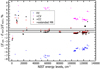Fig. 1. Comparison of computed energy levels using different strategies with data from the NIST database. The solid lines indicate 0.5% deviation from the NIST data.

As we can see from Fig. 1, the largest disagreement with NIST energy levels is for states in the ground configuration, and the difference is up to 3.68%. So in Fig. 2 we represented the convergence of these states using the VV+CV+CC+extended MR strategy. Figure 2 shows that the results do not change after adding more correlations (extending OS₄ to OS₅). This means that convergence is achieved for OS₅. The situation is similar for all other states and energies change by only up to 11 cm⁻¹ when the orbital space is extended from OS₄ to OS₅.

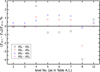Fig. 2. Convergence of the levels of the 4d2 configuration (VV+CV+CC+extended MR strategy). The number of the levels match the order of levels in Table A.1.

The Breit and QED corrections affect the energy spectrum up to 0.8%. The largest contribution, about 5%, is to the 4d^{2 3}F_3,4 states. Figure 3 presents the differences between the NIST energies and final results (VV+CV+CC+extended MR strategy OS₅) of the present work. Root-mean-square (rms) deviations obtained for final energy spectra from the experimental (NIST) data are 250 cm⁻¹ and 520 cm⁻¹ for levels below and above 100 000 cm⁻¹, respectively.

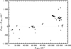Fig. 3. Deviations of the present calculated energy levels (VV+CV+CC+extended MR strategy OS5) from the NIST values.

In Table A.1 the final results obtained using the VV+CV+CC+extended MR computational scheme with OS₅ are presented. The table lists energy spectra and atomic state function composition in LS-coupling for 40 even states of the 4d², 4d5s, 5s², 4d6s, 4d5d, 5p² configurations and for 44 odd states of the 4d5p, 5s5p, 4d6p, 4d4f configurations. The states are given with unique labels (Gaigalas et al. 2017). In the computed spectra there are two states (35 and 56), for which the assigned labels are not based on the largest contribution to the composition. The first state was assigned as 4d5d ³D₃ with 0.35 contribution and the second state as $4\mathrm{d}6\mathrm{p}{}^3{\mathrm{F}}_2^{°}$ with 0.21 contribution to the composition.

The $4\mathrm{d}6\mathrm{p}{}^3{\mathrm{P}}_{0,1}^{°}$ states of the Zr III ion are not given in the NIST database. Our calculated excitation energies for these two states are 119 058 cm⁻¹ (for ${}^3{\mathrm{P}}_0^{°}$) and 118 988 cm⁻¹ (for ${}^3{\mathrm{P}}_1^{°}$). That is in good agreement with the calculated values 119 613 cm⁻¹ and 119 501 cm⁻¹ for the ${}^3{\mathrm{P}}_0^{°}$ and ${}^3{\mathrm{P}}_1^{°}$ states, respectively, given in Reader & Acquista (1997).

3.2. Evaluation of transition data

Transition data of electric dipole, magnetic dipole, and electric quadrupole transitions were computed using wave functions from the VV+CV+CC+extended MR strategy. The accuracy of the electric dipole (E1) and quadrupole (E2) transitions data was evaluated using the dT quantity (Ekman et al. 2014), which is defined as

$$\begin{array}{c}\hfill dT=\frac{|A_{\mathrm{l}}-A_{\mathrm{v}}|}{max(A_{\mathrm{l}},A_{\mathrm{v}})},\end{array}$$(2)

where A_l and A_v are transition rates in length and velocity forms, respectively.

Obtained transition data, such as wavelengths, line strengths, weighted oscillator strengths, transition rates of E1, M1, and E2 transitions, along with the accuracy indicator dT, are given in Table 4. The table also gives experimental wavelengths, adjusted (by experimental wavelengths) transition rates, and uncertainty (as in the NIST database) of each transition. These uncertainties were evaluated by comparing transition rates with experimental values given by Mayo et al. (2005) and estimated using the methods described in Kramida (2013). The full table is available at the CDS.

A scatterplot of dT versus the line strengths is presented in Fig. 4 to show the difference between length and velocity forms of computed E1 transitions. As we can see from the figure for most of the stronger transitions, dT is well below 10%.

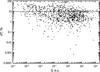Fig. 4. Scatterplot of dT vs. the line strength S of E1 transitions for Zr III. The solid line indicates the 10% deviations.

In Fig. 5 transition rates from experiment (Mayo et al. 2005) are compared with results from this work. As shown in the figure, most of the computed transition rates are smaller than experimental rates. The differences for weaker transitions are much larger than the experimental error bars. The worst disagreement is for four transitions, namely 4d5d ³D₃ (No. 35) – $4\text{d}5\text{p}{ }^3{\text{D}}_2^o$ (No. 19); 4d5d ³D₃ (No. 35) – $4\text{d}5\text{p}{ }^3{\text{F}}_4^o$ (No. 21); $4\text{d}5\text{p}{ }^3{\text{D}}_2^o$ (No. 19) – 4d5s ¹D₂ (No. 13); $4\text{d}5\text{p}{ }^3{\text{D}}_1^o$ (No. 17) – 4d5s ¹D₂ (No. 13).

Lifetimes for the studied levels were computed in length and velocity gauges and the results are presented in Table A.1. Computed lifetimes for some states of the 4d5p configuration are compared with experimental values and other theoretical calculations in Table 2. From this table we can see that the lifetimes obtained in this work agree with the experimental lifetimes within the uncertainties of the latter. Other theoretical lifetimes are lower than the experimental lifetimes by (11–22)%.

We chose five E1 transitions, which contribute significantly to the lifetime of $4\text{d}5\text{p}{ }^1{\text{D}}_2^o$ state, for a deeper analysis. The influence of electron correlations to the line strengths of these five lines is presented in Figs. 6 and 7. As shown in both figures, it is important to include CV and CC correlations in the computations. The line strengths for $4\text{d}5\text{p}{ }^1{\text{D}}_2^o$ – 4d²³F₂, $4\text{d}5\text{p}{ }^1{\text{D}}_2^o$ – 4d5s ³D₁ transitions (Fig. 7) decreases by 1.5 times when CV and CC correlations are included. In Table 3, as an example, line strengths of these five lines are also compared with experimental results and other theoretical computations. Computed line strengths using the VV+CV+CC+extended MR strategy disagree with experimental and other theoretical results. A better agreement with other investigations is achieved when only VV correlations are included.

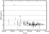Fig. 5. Natural logarithm of the ratio of experimental A-values of Mayo et al. (2005) to the present adjusted (by experimental wavelengths) A-values plotted vs. the present calculated line strength S. The error bars correspond to experimental uncertainties.

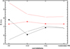Fig. 6. Contributions of electron correlation effects to line strengths (for OS4): $4\text{d}5\text{p}{ }^1{\text{D}}_2^o$ – 4d21D2 (black), $4\text{d}5\text{p}{ }^1{\text{D}}_2^o$ – 4d5s 1D2 (red). Closed and open symbols indicate line strengths in length and in velocity forms, respectively.

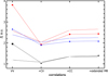Fig. 7. Contributions of electron correlation effects to line strengths (for OS4): $4\text{d}5\text{p}{ }^1{\text{D}}_2^o$ – 4d23F2 (black), $4\text{d}5\text{p}{ }^1{\text{D}}_2^o$ – 4d5s 3D1 (red), and $4\text{d}5\text{p}{ }^1{\text{D}}_2^o$ – 4d5s 3D2 (blue). Closed and open symbols indicate line strengths in length and in velocity forms, respectively.

In Figs. 8 and 9 convergence of line strengths in length and velocity forms using the VV+CV+CC+extended MR strategy is shown. We see that convergence of line strengths in both forms is achieved. The dT for the $4\text{d}5\text{p}{ }^1{\text{D}}_2^o$ – 4d²¹D₂ transition is 0.3% and for $4\text{d}5\text{p}{ }^1{\text{D}}_2^o$ – 4d5s ¹D₂ transition – 10.4% (Fig. 8); the dT values for $4\text{d}5\text{p}{ }^1{\text{D}}_2^o$ – 4d²³F₂, $4\text{d}5\text{p}{ }^1{\text{D}}_2^o$ – 4d5s ³D₁, $4\text{d}5\text{p}{ }^1{\text{D}}_2^o$ – 4d5s ³D₂ transitions are 2.4%, 8.3%, and 7.5%, respectively (Fig. 9).

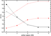Fig. 8. Convergence of line strengths using the VV+CV+CC+extended MR strategy; $4\text{d}5\text{p}{ }^1{\text{D}}_2^o$ – 4d21D2 (black), $4\text{d}5\text{p}{ }^1{\text{D}}_2^o$ – 4d5s 1D2 (red). Closed and open symbols denote line strengths in length and in velocity forms, respectively.

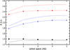Fig. 9. Convergence of line strengths using the VV+CV+CC+extended MR strategy; $4\text{d}5\text{p}{ }^1{\text{D}}_2^o$ – 4d23F2 (black), $4\text{d}5\text{p}{ }^1{\text{D}}_2^o$ – 4d5s 3D1 (red), $4\text{d}5\text{p}{ }^1{\text{D}}_2^o$ – 4d5s 3D2 (blue). Closed and open symbols indicate line strengths in length and in velocity forms, respectively.

4. Conclusions

Energy spectra and transition data of E1, M1, and E2 transitions are presented for Zr III using MCDHF and RCI methods.

Various electron correlation effects were studied. The CV and CC electron correlations are very important in the energy spectra investigations for Zr III ion. The analysis shows that the line strengths for computed transitions are sensitive to CV and CC correlations as well.

The rms deviations obtained for final energy spectra (VV+CV+CC+extended MR strategy OS₅) from the experimental data are 250 cm⁻¹ and 520 cm⁻¹ for levels below and above 100 000 cm⁻¹, respectively.

The computed lifetimes agree with available experimental values within the uncertainties of the latter. The accuracy of the transition rates has been evaluated. About 7% of all E1 transitions have uncertainties of 18% in A values (NIST category C+), 41% have uncertainties of 29% (NIST category D+), 24% have uncertainties of 54% (NIST category D), and only 28% have greater uncertainties corresponding to NIST category E. These estimates should be redone when more experimental data appear considering the reasons given below.

It was observed that there are some disagreements between results of both Mayo papers (Mayo et al. 2006, 2005). By comparing computed lifetimes with measured values from Mayo et al. (2006) they agree within the uncertainties of the experiment. However, when the computed transition rates are compared with the rates presented in Mayo et al. (2005) there is a large disagreement. The disagreement could appear due to the fact that transition probabilities in Mayo et al. (2005) were obtained from the branching ratio measurements and the theoretical lifetime values were calculated in their work but not obtained from experimental measurements. It is impossible to carry out a deeper analysis because these authors did not present the lifetimes to which they normalized their measured branching fractions and did not give A values for the unobserved decay branches. Further studies and measurements are needed to explain these disagreements.

Acknowledgments

This project has received funding from European Social Fund (project No. 09.3.3-LMT-K-712-02-0072) under grant agreement with the Research Council of Lithuania (LMTLT). Part of large-scale computations were performed at the High Performance Computing Center “HPC Sauletekis” of the Faculty of Physics at Vilnius University.

References

Appendix A: Atomic state function composition in LS-coupling, energy levels, and lifetimes for the Zr III ion.

All Tables

All Figures

	Fig. 1. Comparison of computed energy levels using different strategies with data from the NIST database. The solid lines indicate 0.5% deviation from the NIST data.
In the text

	Fig. 2. Convergence of the levels of the 4d2 configuration (VV+CV+CC+extended MR strategy). The number of the levels match the order of levels in Table A.1.
In the text

	Fig. 3. Deviations of the present calculated energy levels (VV+CV+CC+extended MR strategy OS5) from the NIST values.
In the text

	Fig. 4. Scatterplot of dT vs. the line strength S of E1 transitions for Zr III. The solid line indicates the 10% deviations.
In the text

	Fig. 5. Natural logarithm of the ratio of experimental A-values of Mayo et al. (2005) to the present adjusted (by experimental wavelengths) A-values plotted vs. the present calculated line strength S. The error bars correspond to experimental uncertainties.
In the text

	Fig. 6. Contributions of electron correlation effects to line strengths (for OS4): $4\text{d}5\text{p}{ }^1{\text{D}}_2^o$ – 4d21D2 (black), $4\text{d}5\text{p}{ }^1{\text{D}}_2^o$ – 4d5s 1D2 (red). Closed and open symbols indicate line strengths in length and in velocity forms, respectively.
In the text

	Fig. 7. Contributions of electron correlation effects to line strengths (for OS4): $4\text{d}5\text{p}{ }^1{\text{D}}_2^o$ – 4d23F2 (black), $4\text{d}5\text{p}{ }^1{\text{D}}_2^o$ – 4d5s 3D1 (red), and $4\text{d}5\text{p}{ }^1{\text{D}}_2^o$ – 4d5s 3D2 (blue). Closed and open symbols indicate line strengths in length and in velocity forms, respectively.
In the text

	Fig. 8. Convergence of line strengths using the VV+CV+CC+extended MR strategy; $4\text{d}5\text{p}{ }^1{\text{D}}_2^o$ – 4d21D2 (black), $4\text{d}5\text{p}{ }^1{\text{D}}_2^o$ – 4d5s 1D2 (red). Closed and open symbols denote line strengths in length and in velocity forms, respectively.
In the text

	Fig. 9. Convergence of line strengths using the VV+CV+CC+extended MR strategy; $4\text{d}5\text{p}{ }^1{\text{D}}_2^o$ – 4d23F2 (black), $4\text{d}5\text{p}{ }^1{\text{D}}_2^o$ – 4d5s 3D1 (red), $4\text{d}5\text{p}{ }^1{\text{D}}_2^o$ – 4d5s 3D2 (blue). Closed and open symbols indicate line strengths in length and in velocity forms, respectively.
In the text

References

- Beck, D. R., & Pan, L. 2004, Phys. Scr., 69, 91 [NASA ADS] [CrossRef] [Google Scholar]
- Castelli, F., Cowley, C. R., Ayres, T. R., Catanzaro, G., & Leone, F. 2017, A&A, 601, A119 [NASA ADS] [CrossRef] [EDP Sciences] [Google Scholar]
- Charro, E., López-Ayuso, J. L., & Martín, I. 1999, J. Phys. B: At. Mol. Opt. Phys., 32, 4555 [NASA ADS] [CrossRef] [Google Scholar]
- Dyall, K., Grant, I., Johnson, C., Parpia, F., & Plummer, E. 1989, Comput. Phys. Commun., 55, 425 [NASA ADS] [CrossRef] [Google Scholar]
- Ekman, J., Godefroid, M., & Hartman, H. 2014, Atoms, 2, 215 [NASA ADS] [CrossRef] [Google Scholar]
- Froese Fischer, C., Godefroid, M., Brage, T., Jönsson, P., & Gaigalas, G. 2016, J. Phys. B: At. Mol. Opt. Phys., 49, 182004 [NASA ADS] [CrossRef] [Google Scholar]
- Froese Fischer, C., Gaigalas, G., Jönsson, P., & Bieroń, J. 2019, Comput. Phys. Commun., 237, 184 [NASA ADS] [CrossRef] [Google Scholar]
- Gaigalas, G., Žalandauskas, T., & Rudzikas, Z. 2003, At. Data Nucl. Data Tables, 84, 99 [NASA ADS] [CrossRef] [Google Scholar]
- Gaigalas, G., Froese Fischer, C., Rynkun, P., & Jönsson, P. 2017, Atoms, 5, 6 [NASA ADS] [CrossRef] [Google Scholar]
- Grant, I. P. 2007, Relativistic Quantum Theory of Atoms and Molecules (New York: Springer) [CrossRef] [Google Scholar]
- Kramida, A. 2013, Fusion Sci. Technol., 63, 313 [CrossRef] [Google Scholar]
- Kramida, A., Ralchenko, Yu., Reader, J., & NIST ASD Team 2019, NIST Atomic Spectra Database (ver. 5.7.1), [Online] (Gaithersburg, MD: National Institute of Standards and Technology), Available: https://physics.nist.gov/asd [2019, November 14] [Google Scholar]
- Leckrone, D. S., Johansson, S., Wahlgren, G. M., & Adelman, S. J. 1993, Phys. Scr., T47, 149 [NASA ADS] [CrossRef] [Google Scholar]
- Martins, M. C., Santos, J. P., Costa, A. M., & Parente, F. 2006, Eur. Phys. J. D - At. Mol. Opt. Plasma Phys., 39, 167 [Google Scholar]
- Mayo, R., Ortiz, M., & Campos, J. 2005, J. Quant. Spectr. Radiat. Trans., 94, 109 [NASA ADS] [CrossRef] [Google Scholar]
- Mayo, R., Campos, J., Ortiz, M., et al. 2006, Eur. Phys. J. D, 40, 169 [NASA ADS] [CrossRef] [EDP Sciences] [Google Scholar]
- Pandey, G., Lambert, D. L., Rao, N. K., & Jeffery, C. S. 2004, ApJ, 602, L113 [NASA ADS] [CrossRef] [Google Scholar]
- Reader, J., & Acquista, N. 1997, Phys. Scr., 55, 310 [NASA ADS] [CrossRef] [Google Scholar]
- Redfors, A. 1991, A&A, 249, 589 [NASA ADS] [Google Scholar]
- Sikström, C. M., Lundberg, H., Wahlgren, G. M., et al. 1999, A&A, 343, 297 [NASA ADS] [Google Scholar]