| Issue |
A&A
Volume 637, May 2020
|
|
|---|---|---|
| Article Number | A79 | |
| Number of page(s) | 8 | |
| Section | Planets and planetary systems | |
| DOI | https://doi.org/10.1051/0004-6361/201937045 | |
| Published online | 19 May 2020 | |
Quantitative assessment of water content and mineral abundances at Gale crater on Mars with orbital observations
1
State Key Laboratory of Space Weather, National Space Science Center, Chinese Academy of Sciences,
Beijing,
100190,
PR China
e-mail: This email address is being protected from spambots. You need JavaScript enabled to view it.
2
Center for Excellence in Comparative Planetology, Chinese Academy of Sciences,
Hefei,
PR China
3
University of Glasgow,
Scotland,
UK
4
University of Chinese Academy of Science,
Beijing
100049,
PR China
Received:
3
November
2019
Accepted:
10
April
2020
Abstract
Context. The information of water content can help to improve atmospheric and climate models, and thus provide a better understanding of the past and present role of water and aqueous alteration on Mars. Mineral abundances can provide unique constraints on their formation environments and thus also on the geological and climate evolution of Mars.
Aims. In this study, we used a state-of-the-art approach to derive the hydration state and mineral abundances over Gale crater on Mars, analysing hyperspectral visible/near-infrared data from the Observatoire pour la Minéralogie, l’Eau, les Glaces et l’Activité (OMEGA) instrument onboard Mars Express and from the Compact Reconnaissance Imaging Spectrometer for Mars (CRISM) instrument onboard the Mars Reconnaissance Orbiter.
Methods. The Discrete Ordinate Transfer model was used to perform atmospheric and thermal correction of the OMEGA and CRISM hyperspectral data in order to derive the surface single scattering albedos (SSAs) at Gale crater, Mars. Water content was estimated using a linear relationship between the derived effective single-particle absorption thickness at 2.9 μm from SSAs and the water weight percentage. Mineral abundances were retrieved by performing the linear spectral unmixing of SSAs from CRISM data. The results were compared with the ground-truth results returned from Curiosity rover.
Results. The water content for most areas at Gale crater derived using the OMEGA data is around 2–3 water weight percent (water wt % hereafter), which is in agreement with that derived from the in situ measurements by Curiosity’s Sample Analysis at Mars instrument. However, the sensitivity tests show that uncertainties exist due to the combination of several factors including modelling bias, instrumental issue, and different sensing techniques. The derived mineral abundances using the orbital data are not fully consistent with that derived by Curiosity, and the discrepancy may be due to a combination of dust cover, texture, and particle size effects, as well as the effectiveness of the quantitative model.
Conclusions. The ground-truth data from Curiosity provide a critical calibration point for the quantitative method used in the orbital remote-sensing observations. Our analysis indicates that the method presented here has great potential for mapping the water content and mineral abundances on Mars, but caution must be taken when using these abundance results for geological interpretations.
Key words: publications, bibliography / radiative transfer / planets and satellites: surfaces / infrared: planetary systems / techniques: spectroscopic / methods: data analysis
© ESO 2020
1 Introduction
In situ explorations of Mars by landers and rovers can provide highly detailed information on the geology and mineralogy of Mars on a regional scale, yet orbital remote sensing is still the main approach used to study Mars as a whole. One important objective of the orbital remote sensing analyses is to characterize mineral species in both a qualitative and quantitative way using the reflectance spectroscopy technique. In particular, the relative abundances of the single minerals in the mineral assemblages can provide unique constraints on their formation environments and thus also on the geological and climate evolution of Mars. In addition to mineral species, water content is also an important parameter on Mars, as water abundance can help to improve atmospheric and climate models and provide a better understanding of the past and present role of water and aqueous alteration on Mars. Different methods have been developed to quantify mineral abundances. Quantitative analyses have been performed by various authors to derive mineral abundances at visible, near-infrared (NIR), and thermal-infrared wavelengths (Ramsey & Christensen 1998; Combe et al. 2008; Rogers & Aharonson 2008; Poulet et al. 2009, 2014; Goudge et al. 2015; Edwards & Ehlmann 2008; Lin et al. 2016; Liu et al. 2016; Salvatore et al. 2018). Also, water content on Mars has been evaluated in several studies (e.g. Milliken et al. 2007; Audouard et al. 2014), but it is always difficult to evaluate the accuracy of the models. Several factors could affect the model accuracy of mineral abundances, including the radiative transfer model used to retrieve surface albedos, spectral unmixing model, endmember selections, optical constant uncertainties, grain size selections, and observational bias, and so on. A detailed discussion on the potential model uncertainties can be found in Liu et al. (2016). The ground truth data acquired by lander and rover missions are particularly important for evaluating the quantitative inversion models that are applied to orbital remote-sensing data, but the quantitative results from in situ and orbital observations have not been compared. The Mars Science Laboratory (MSL) Curiosity rover provides an excellent opportunity to test the quantitative models.
The Curiosity rover has travelled more than 21 km on the surface of Mars since it began to explore Gale crater on August 6, 2012. Gale crater is located on fluvial dissected highland terrain at the dichotomy boundary on Mars, with a mountain of 5 km in height (Aeolis Mons) formed by deposition, burying, lithification, exhumation, and erosion of sedimentary rocks around 3.1–3.3 Gyr ago (Grotzinger et al. 2015). One of the primary goals of the mission is to investigate early Hesperian-aged sedimentary rocks on the lower slopes of Aeolis Mons (i.e. Mount Sharp). Orbital remote sensing data have shown a variety of minerals including phyllosilicates, sulfates, and hematite in these rocks, suggesting changes in ancient aqueous environments (Milliken et al. 2010; Fraeman et al. 2016). Phyllosilicates have long been a priority target for in situ exploration by Curiosity, as these minerals can be key indicators of habitable environments and may help preserve organic compounds (Farmer & Des Marais 1999; Grotzinger et al. 2014; Bristow et al. 2015). Hydrated sulfates are lying stratigraphically above clay minerals over hundreds of meters of stratigraphy, and this sequence may record a large-scale change from wetter to more arid environments on the surface (Milliken et al. 2010). After exploring the Bradbury group on the plains of Gale crater (Aeolis Palus), Curiosity drove through ~350 m of vertical stratigraphyto investigate the Murray formation of Mount Sharp, and is currently performing an in situ analysis over the clay-bearing units.
The sedimentology, geochemistry, and mineralogy of the sedimentary rocks investigated by a suite of instruments on Curiosity provide plentiful evidence for deposition in an active aqueous environment such as fluvial and lacustrine processes at Gale crater (Grotzinger et al. 2015). Elemental abundances from the ChemCam and APXS instruments are evaluated for bedrock targets, and mineralogical information for drilled bedrock targets is provided by the CheMin (XRD) instrument (Blake et al. 2012). These quantitative measurements can be used to compare with the mineral abundance information acquired by the visible–NIR spectral reflectance data from orbital remote sensing data. The Sample Analysis at Mars (SAM) instrument onboard Curiosity provides diverse analytical capabilities for exploring Martian materials, including volatile compositions such as water (Mahaffy et al. 2012). These quantitative results of water content can be used to compare results derived from orbital spectral data by evaluating the 2.9 μm water band. Thus, the ground truth data acquired by Curiosity rover provide an excellent opportunity to validate the quantitative analysis results acquired from orbital instruments.
In this work, we use the Discrete Ordinate Radiative Transfer (DISORT) code (Stamnes et al. 1988) to perform atmosphericcorrection on the visible and infrared spectral data from the Observatoire pour la Minéralogie, l’Eau, les Glaces et l’Activité (OMEGA) instrument (Bibring et al. 2005) onboard Mars Express and from the Compact Reconnaissance Imaging Spectrometer for Mars (CRISM) instrument (Murchie et al. 2007) onboard the Mars Reconnaissance Orbiter (MRO). By applying the Hapke bidirectional reflectance model to simulate Mars surface scattering properties, we retrieve the single scattering albedos over Gale crater from OMEGA and CRISM I/F data. Watercontent over Gale crater was assessed by evaluating the broad absorption at the wavelength of 2.9 μm in the OMEGA single scattering albedo spectra. Mineral abundances over Curiosity’s traverse at Gale are retrieved from CRISM single scattering albedo spectra. Finally, we use the quantitative results from Curiosity’s in situ observations to compare with the water content and mineral abundances at Gale crater derived from orbital observations, and evaluate the accuracy of our quantitative inversion model.
2 Data sets and methodology
2.1 Data sets
The data sets used in this study include OMEGA and CRISM hyperspectral data. OMEGA spectrometer operates in the spectral range from NIR to visible frequencies, with 352 contiguous spectral channels over three main spectrometers: visible–near-infrared spectrometer (VNIR) with 92 channels ranging between 0.35 and 1.05 μm; spectrometer C with 128 channels ranging between 0.97 and 2.73 μm, and spectrometer L with 128 channels ranging between 2.55 and 5.1 μm. OMEGA has a varied spatial resolution ranging between 300 m and 3 km per pixel, depending on the altitude of the orbiter when the image was taken. CRISM spectrometer comprises 544 channels ranging between 0.36 and 3.92 μm. The spatial resolution is far greater in CRISM, and the surface of Mars can be sampled in two ways: “full-resolution targeted” (FRT; regularized to 18 m pixel−1) and “half-resolution long” and short (HRL/HRS; regularized to 36 m pixel−1; Murchie et al. 2007).
2.2 Atmospheric correction of OMEGA and CRISM I/F data
The OMEGA and CRISM I/F values at the top of Martian atmosphere contain radiative contributions from both the surface and atmosphere,including gas and aerosol absorption, scattering, and emission. These components could affect the shape of the spectra and could also obscure the diagnostic absorption bands of minerals on the surface of Mars. To retrieve the surface reflectance, these atmospheric contributions need to be removed. The traditional method is to use the simple “volcano scan” correction method of removing atmospheric gas absorptions in order to retrieve surface spectra. Volcano scan correction attempts to minimise atmospheric gas absorption features by dividing each I/F spectrum by a scaled atmospheric transmission spectrum (Bibring et al. 2005; Langevin et al. 2005; Mustard et al. 2005). The volcano scan method does not account for either atmospheric gas variations such as H2O to CO2 ratio changes or the scattering effects of atmospheric aerosols, which can lead to errors in identifying subtle absorption features that have been masked by minor variations in aerosol scattering and absorption (Wiseman et al. 2016). In this study, we use the Discrete Ordinate Radiative Transfer (DISORT) model to simulate the radiative contributions from both surface and atmosphere simultaneously (Stamnes et al. 1988; Wolff et al. 2009).
To atmospherically correct OMEGA and CRISM data, the DISORT model is used to first simulate the I/F at OMEGA and CRISM band passes from the top of the Mars atmosphere by including radiative contributions from both the atmosphere and the surface. For each OMEGA and CRISM channel, I/F is modelled as a function of viewing geometry, atmospheric properties, surface scattering parameters, and solar irradiance scaled to the appropriate heliocentric distance for the given observation. The input atmospheric properties include dust and ice aerosol optical depths, water vapour abundance, atmospheric pressure and temperatureprofiles, and surface pressure. Temperatures and pressure for each layer of the atmosphere, dust and ice aerosol radiative properties, and water vapour abundance were estimated from historical climatology trends based on Thermal Emission Spectrometer (TES) data at the latitude, longitude, and solar longitude (Ls) when OMEGA data were collected (Conrath et al. 2000; Smith 2004). The aerosol optical depths used in CRISM data modelling were derived based on the CRISM emission phase function (EPF) corresponding to the CRISM data to be analysed (Wolff et al. 2009).
The surface scattering properties at the lower boundary within the DISORT is modelled with the Hapke bidirectional reflectance distribution function (BRDF; Hapke 2012b). The Hapke bidirectional reflectance function is described by the following equation (Hapke 2012b):
![Mathematical equation: \begin{align*} rf(i,e,g) \;{=}\; & \frac{w}{4}\frac{\mu_0}{\mu_0+\mu}\left\{[1+B(g)]p(g)\right.\nonumber\\[2pt] &\left.+\,H(\mu_0)H(\mu)-1\right\}S(i,e,g), \end{align*}](/articles/aa/full_html/2020/05/aa37045-19/aa37045-19-eq1.png) (1)
(1)
where rf(i, e, g) is the radiance factor, equivalent to CRISM I/F; i, e, g are incidence, emergence, and phase angles, respectively; μ0 is the cosine of the effective incidence angle and μ is the cosine of the effective emergence angle, which are used to describe effective tilt of the surface; ω is the average single particle scattering albedo defined as the ratio of scattering efficiency to the sum of scattering and absorption efficiencies, and is the primary scattering parameter to be retrieved; P(g) is the surface phase function describing the angular distribution of light intensity scattered by a single particle; B(g) is the opposition effect describing the sharp surge in brightness around the zero phase angle; H is the multiple scattering function; and S is the shadowing function defined by a macroscopic roughness parameter,  . Following previous studies (Wolff et al. 2009; Liu et al. 2016), we used an asymmetry parameter b of 0.3, forward-scattering fraction c of 0.6, opposition surge amplitude B0 of 1.0, width of opposition surge h of 0.06, and roughness parameter
  of 15.0. We note that Vincendon (Vincendon et al. 2013) derives a mean BRDF representative of widespread typical Martian terrains constrained by orbital observations and provides a parameterisation of a new set of mean Mars surface phase functions based on Hapke formalism. These values are important for cross comparisons in the future validation of the model.
2.3 Thermal correction of OMEGA data and water content calculation
In addition to atmospheric contributions, OMEGA L spectrometer I/F data contain thermal emission contributions at wavelengths between 2.8 and 5.1 μm. To retrieve surface reflectance at these wavelengths, the thermal emission contribution needs to be removed. According to Planck’s law, thermal emission is a function of the temperature of the materials. Therefore, to properly model the thermal emission contribution, the kinetic temperatures of the surface of Mars need to be calculated. Following previously developed methods (Milliken et al. 2007; Liu et al. 2012), we first used the DISORT model to retrieve the reflectance at 2.5 μm by performing the atmospheric correction of OMEGA C spectrometer data. The linear relationship between reflectance values at 2.5 and 5.0 μm was used to estimate the reflectance values at 5.0 μm (Jouglet et al. 2007; Milliken et al. 2007). Based on Kirchhoff’s rule (emissivity = 1-reflectance), we can estimate the temperatures by fitting a black body curve over the thermally emitted radiance. The retrieved temperature for each pixel was then used as the input parameter in the DISORT model to simulate the thermal emission contribution (in addition to atmospheric contribution) to OMEGA I/F data. The surface single scattering albedo between 2.8 and 5.1 μm was then retrieved using the look-up table approach.
At NIR wavelengths, water (including absorbed and structurally bonded water) has an absorption band around 2.9–3.0 μm, and the strength of this band can be used to characterise the abundance of water. Previous studies have shown that water content can be obtained using a linear relationship between the effective single-particle absorption thickness (ESPAT) at 2.9 μm and water weight percentage (Milliken et al. 2005). The ESPAT function (Hapke 2012a) is calculated by
 (2)
(2)
where w is the single scattering albedo. Here we used the continuum-removed single scattering albedo spectra following Milliken & Mustard (2007a). The water weight percentage of many Martian regolith analogues can be approximated by a linear function:
 (3)
(3)
where the value of “A” may vary depending on the composition and grain size of analogous Martian materials, and here we used a linear coefficient of 4.17 for “A” following Audouard et al. (2014). The model yields an accuracy of 1 wt.% H2O for a wide range of albedo values and compositions (Milliken & Mustard 2007a).
2.4 Mineral abundance retrieval from CRISM data
One fundamental challenge and important aspect of planetary remote sensing analysis is accurately estimating mineral abundances from VNIR data. The CRISM single scattering albedos (SSA) derived from the DISORT modelling were used to perform a spectral unmixing analysis. Single scattering albedos of individual components can be added linearly to make the mixed SSAs using the following equation (Hapke 1981):
 (4)
(4)
where Mi is the mass fraction, ρi is the density, Di is the average effective particle size, and ωi is the single scattering albedo for the ith end member. As compared to the traditional non-linear unmixing of VNIR data, the linear unmixing of SSAs can avoid complex interactions caused by several material properties, including the abundance, grain size, and texture of each individual surface component (Nash & Conel 1974; Singer 1981; Clark 1983; Johnson et al. 1992). Therefore, the use of the DISORT model to derive SSAs that can be linearly unmixed can greatly improve the accuracy of mineral abundance models.
To do spectral unmixing, a SSA spectral library is needed. SSA is dependent on the optical constants, which were first obtained using the Shkuratov or Hapke radiative transfer model (Shkuratov et al. 1999; Martone et al. 2014; Sklute et al. 2015). Single scattering albedos were then calculated based on the Hapke model for a given grain size using the following equation:
 (5)
(5)
where Se is the reflectivity for the external incident light and is a function of both n and k:
 (6)
(6)
and Si is the reflectivity for the internal incident light and is expressed as:
 (7)
(7)
where Θ is the particle internal transmission coefficient, and is defined as:
 (8)
(8)
where D is the particle diameter (grain size), and ri is the internal diffuse reflectance inside the particle, defined as:
 (9)
(9)
and α is the absorption coefficient for the internal attenuation, defined as:
 (10)
(10)
In Eqs. (8) and (9), parameter denotes the internal volume scattering coefficient. Lucey (1998) found that a value of zero gives an adequate fit to the data from particulate mineral samples. In this study, we set the value of s to zero.
In the spectral unmixing analysis, CRISM SSAs were modelled using the non-negative least squares (NNLS) linear deconvolution unmixing algorithm (Lawson et al. 1974; Rogers & Aharonson 2008). For each CRISM SSA spectrum, the model must reproduce the shape and depth of each of the absorption bands, the spectral continuum, and the absolute value of the reflectance. CRISM SSA spectra were modelled through several iterations to produce the best mathematical and visual fit, and mineral abundances and grain sizes for each spectrum were provided by optimising for the lowest root mean square (RMS) error between the retrieved and the modelled single scattering albedos.
3 Results and discussion
3.1 Temperature and water content at Gale crater
As described in Sect. 2.3, water content can be estimated using a linear relationship between ESPAT at 2.9 μm and water weight percentage. ESPAT at 2.9 μm is a function of the SSA at 2.9 μm, where SSA has been corrected for the thermal contribution using the surface temperatures at Gale crater derived from the OMEGA data. Figures 1a and b show the mosaic maps of surface kinetic temperatures and water weight percentage per unit mass, respectively, covering a large area including Gale crater. We note the mosaic maps are from three different OMEGA observations, and therefore these maps are time (i.e. season and time of the day during the observation)dependent (Table 1). The temperatures in Fig. 1a range between ~210 and ~280 K. At the samelatitude, the temperature varies significantly for the three observations, mostly due to the differences of the observation time. For the same observation, the temperature differences are strongly correlated with the physical properties (i.e. grain size and porosity, etc.) of the materials, and thus this can help us to understand the nature of the materials of the study area. The water content map in Fig. 1b shows latitude dependency in general, i.e. the area with higher latitude has higher water content. The trend is consistent with the results of Milliken et al. (2007) showing that the largest spatial variations in H2O occur as a function of latitude.
The zoomed maps over Gale crater for albedo, temperature, and water content, respectively, are shown in Fig. 2, and these maps contain two OMEGA swaths, namely ORB2363_4 (left) and ORB0436_2 (right). The area in ORB2363_4 swath with higher temperatures on the western crater floor shown in Fig. 2b corresponds to the low-albedo area in Fig. 2a. The area is mostly composed of dark sand dunes, and the temperature can reach as high as 280 K. The temperature difference between this area and the surroundings indicates the different physical property of materials. A previous study using the ground-truth data from Curiosity showed that the dark sand on the western crater floor has relatively low thermal inertia (Vasavad et al. 2017). The thermal inertia represents the resistance ofsurface materials to temperature change during a full heating/cooling cycle. The observation time for ORB2363_4 is 11:00 AM local time on Mars, so it is not surprising that the sand dune materials with low thermal inertia were heated quicker than the surrounding materials and therefore have higher temperatures. Thus, the observed temperature variations at Gale crater can be explained by physical properties of the materials obtained by the ground-truth observations. Similar to the temperature map, the dark sand dunes in the western crater floor area have higher water content than the surroundings (Fig. 2c), with a value up to ~3–4 wt%. The SampleAnalysis at Mars instrument Evolved Gas Analyser (SAM-EGA) detected evolved water and many other volatile species along Curiosity’s traverse at Gale crater (Meslin et al. 2013; Sutter et al. 2017). As of sol 1237 (29 January 2016), 11 sampling sites have been examined by SAM, of which two eolian dune samples of differing particle size distribution were scooped from Gobabeb (GB1 and GB2). Gobabeb, as a part of the “Bagnold Dune Field”, are loose, unconsolidated modern eolian sediments that overlie the Yellowknife Bay and Murray formations, respectively (Grotzinger et al. 2015). The results from the SAM analysis of the samples at Gobadeb indicate that the water content of these eolian sediments is around 1.0 ± 0.5 wt% (Sutter et al. 2017), which is significantly less than that was derived from OMEGA observations (3–4 ± 0.5 wt%). The estimation of water content from the OMEGA data was based on the strong linear correlation between the ESPAT parameter and water contents at ~2.9 μm. The ESPAT is a function of SSA, and a decreasing SSA value signifies an increasing the ESPAT value (see Eq. (2)). The retrieved OMEGA SSAs over the low albedo areas (mostly containing dark sand dunes) and the surrounding areas are shown in Fig. 3, and it is clear that the SSAs over the former are significantly lower than those over the latter. The lower SSA value results in the increasing ESPAT value and thus the higher water content over the dark sand dunes. As noted by Milliken & Mustard (2007b), ESPAT is not necessarily an accurate predictor of low water contents for dark materials. This is because in the low-albedo spectra, the water bands are almost saturated, and small differences between low albedo values can result in large differences in SSA and thus large water content variations. Therefore, our estimate of water content over the dark sand dune area using the OMEGA data may not be accurate due to the low-albedo nature of these materials.
For the area outside the low-albedo areas, the water content we estimated using the OMEGA data is ~2–3 ± 0.5 wt%. The in situ heating experiment measurements of the Rocknest sand shadow materials by the SAM instrument onboard Curiosity yield a bulk water content result of 1.5–3 wt% H2O (Leshin et al. 2013). As investigated in Sutter et al. (2017), nine samples were acquired from sedimentary rocks using a drill and were analysed by SAM-EGA. These samples were found to have a water content of ~2 wt%. These in situ measurements are consistent with the water content estimated by OMEGA data in this work. Audouard et al. (2014) also estimated the water content over Gale crater using the same set of OMEGA data, and these authors found the water content to be around 4–5 wt% which is higher than the value estimated in the present study and in situ measurements by the SAM instrument. There are several possible reasons for the discrepancy in the derived water content between Audouard et al. (2014) and this study: Audouard et al. (2014) may not have accounted for the influence of aerosols in their atmospheric correction of OMEGA data whereas the DISORT model did.
To test how the atmospheric dust aerosols affect the derived water abundance, we reprocessed OMEGA data using the DISORT model assuming a series of dust optical depths. The retrieved single scattering albedo between 1.0 and 4.0 μm at the given dust optical depth is shown in Fig. 4. Higher dust optical depth values indicate more dust contribution was removed in the modelling. The results clearly show that the retrieved single scattering albedos decrease with increasing dust optical depth used in the model, which is consistent with what has been observed by Vincendon et al. (2013). We also derived the corresponding water contents for each of the dust optical depth circumstances. The results shown in Fig. 5 show a clearincrease in water content with increasing dust optical depth (i.e. more dust contribution to be removed). This is not surprising because lower dust optical depth would yield a higher single scattering albedo at all wavelengths including the 3.0 μm region (Fig. 4), which would give a lower ESPAT value and thus lower water content. Therefore, the relationship between dust optical depth used in the DISORT model and water content shown in Fig. 5 is similar to what is shown in Fig. 9 of Audouard et al. (2014). Thus, our analysis indicates that dust aerosol is not the main factor that causes the discrepancy in derived water content between our study and that of Audouard et al. (2014).
Another possible reason for the difference in derived water content using OMEGA data is that here we used a different correction method for atmospheric gases from what was used by these latter authors. In Audouard et al. (2014), OMEGA spectra were corrected for atmospheric attenuation through division by a power-scaled transmission spectrum of the Martian atmosphere,whereas a correlated-k approach was used to correct atmospheric gases in our DISORT modelling. The different methods used for correcting atmospheric gases may cause differences in the retrieved single scattering albedo and thus the water content. Finally, another possible cause of the discrepancy is the difference in surface reflectance models used in these two studies. (Audouard et al. 2014) assumed an isotropic phase function (i.e. p(g) = 1) and no opposition effect (B(g) = 0). In our study, we used the two-termed Henyey-Greenstein phase function, and the opposition effect was not set to zero (see details in Sect. 2.2). The use of a different reflectance model may have induced different single scattering albedos and thus water content.
Therefore, differences in the modelling approach, the modeling bias, or the instrumentation may have caused the discrepancy among the water contents derived from Curiosity by Audouard et al. (2014) and this study. Our analysis also indicates that dust aerosol is quite sensitive to the derived water content. Because elucidation of the exact atmospheric conditions during OMEGA observations is challenging, using the dust optical depths from either the TES climatology database or the Mars Exploration Rovers database can potentially cause inaccurate water content derivation. Using the DISORT radiative transfer model to derive water content in this work is complementary to that of Audouard et al. (2014), and our results indicate that caution must be taken when making geological interpretations of quantitative results derived from orbital observations.
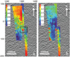 |
Fig. 1 Panel a: Mosaic map of surface kinetic temperature over Gale crater and the surrounding area. The data sets used include: ORB0469_3 (left swath, image acquired at local time 9:00 am, Ls = 42.0), 2363_4 (centre swath, image acquired at local time 11:10 am, Ls = 324.4), 0436_2 (right swath, image acquired at local time 9:30 am, Ls = 37.9). The black box indicates the location of Gale crater and the outline for Fig. 2. Panel b: Mosaic map for water percentage per mass unit (wt%) over Gale crater and the surrounding area. |
OMEGA observations used in this work.
 |
Fig. 2 Panel a: Mosaic map of surface albedo at 1.52 μm over Gale crater. Panel b: Zoomed mosaic map of surface kinetic temperature over Gale crater from Fig. 1. Panel c: Zoomed mosaic map of water percentage per mass unit over Gale crater from Fig. 1. |
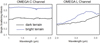 |
Fig. 3 OMEGA single scattering albedo over the dark and bright terrains within Gale crater. The locations of the spectra are indicated in Fig. 2, i.e. “a” represents where the spectrum was taken on the bright terrain, and “b” represents where the spectrum was taken on the dark terrain. |
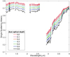 |
Fig. 4 Derived single scattering albedo over the same area with a 10 × 10 pixel size in OMEGA ORB0436_2 assuming different dust optical depths in the DISORT modelling. |
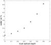 |
Fig. 5 Derived water content as a function of dust optical depth. The uncertainty is around 0.5 wt%. The dust optical depths are the parameters used in the DISORT model, representing how much dust would be removed for the atmospheric correction. |
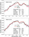 |
Fig. 6 Examples of spectral unmixing results for hydrated sulfate and phyllosilicate-rich terrains. The values after mineral names represent grain sizes, and values with % represent abundance. The RMS errors are also indicated. |
3.2 Mineral abundance at Gale Crater
Gale crater hosts a variety of minerals that formed in a water-rich environment, including phyllosilicates, sulfates, and hematite, which suggests changes in ancient aqueous environments. After exploring the top of Vera Rubin Ridge (VRR) in 2018, which mostly contains hematite signatures, the rover descended into a trough south of the ridge, dropping as much as 15 meters in elevation during the spring of 2019 to explore part of the clay-bearing unit, and Curiosity is currently investigating the clay-bearing unit on the side of Mount Sharp. Elemental abundances and mineralogical information has been obtained from the ChemCam, APXS, and CheMin instruments, which allows us to directly test the quantitative results from the orbital remote sensing data.
Spectral unmixing modelling was performed on the CRISM single scattering albedo spectra to extract the abundances and grain sizes of both hydrous and anhydrous phases. Examples of spectral unmixing results over the hydrated sulfate and phyllosilicate units are shown in Fig. 6. To investigate the spatial distribution of the secondary mineral abundances, we applied our spectral unmixing model to CRISM image HRL0000BABA to generate the mineral abundance map. Figure 7a shows the distribution of the secondary phases mapped over Mount Sharp using the CRISM parameter map (Milliken et al. 2010), and Fig. 7b shows the results of the spectral unmixing analysis over the selected region enclosed in the white box in Fig. 7a. From Fig. 7b it is possible to resolve the hematite, phyllosilicate, and hydrated sulfate unit, and these units are consistent with the spatial distribution derived from the CRISM parameter map shown in Fig. 7a. The spectral unmixing of the CRISM image cube over Gale indicates that there is 30% hematite, 5% phyllosilicates, and 20% hydrated sulfates. We note that the error of the retrieved abundance is around 5% following the error analysis approach used in Liu et al. (2016).
The derived mineral abundances from CRISM observations can be used to compare with the ground-truth data. Vera Rubin ridge (VRR) of Gale crater has the strongest spectral signature consistent with hematite detected from orbit, and the area has been explored by Curiosity rover intensively. Curiosity data show that hematite is present throughout most of the Murry formation and VRR, though it is more abundant in certain drill samples (Rampe et al. 2019). The abundance of these iron oxides are around 20 wt%, as inferred from ChemCam and APXS instruments (Milliken et al. 2019), and the value is slightly lower than what we derived from orbital data. In addition to abundance discrepancies, spatial distribution also shows inconsistencies. For example, orbital data show that hematite is present in only part of the Murry formation, whereas ground-truth data indicate hematite is found throughout most of the Murry formation. Also, orbital data show that the VRR unit, as compared to the Murry formation unit, is mostly enriched in hematite,but the ground-truth data indicate Murry formation and VRR units have a similar abundance of hematite.
In regards to phyllosilicates, our analysis using CRISM orbital data shows an abundance of only ~5% in most clay-rich areas. In contrast, the abundance of clay minerals detected by Curiosity is up to ~28 wt% of the bulk rock (Vaniman et al. 2014; Bristow et al. 2015, 2018; Rampe et al. 2017). Clay-bearing rocks have been detected along Curiosity’s traverse in both the Yellowknife Bay and Murray formations (Vaniman et al. 2014; Bristow et al. 2018; Mangold et al. 2019), but orbital phyllosilicate signatures are mostly absent along the traverse to Curiosity’s current site, the “clay-bearing unit”, as identified from the orbit. The large discrepancies between the orbital and ground-truth data may be due to a combination of dust cover, texture, and particle size effects. Also, the quantitative model used to retrieve mineral abundance is clearly not perfect and needs to be validated and improved using laboratory mixing experiments. The upcoming in situ analysisof the overlying “sulfate unit” will provide an additional opportunity to make a direct comparison between orbital and ground-truth results and further test the quantitative modelling approach using the orbital data.
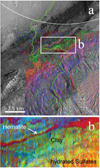 |
Fig. 7 Panel a: CRISM FRT0000BABA RGB mineral parameter map (red = Fe-minerals, green = Fe/Mg-clay minerals, blue = sulfates) overlain on CTX mosaic. Image adapted from Fig. 3a of Milliken et al. (2010). Panel b: Derived mineral abundance map over a region covering Curiosity’s traverse, outlined in the white box in Fig. 7a. |
4 Conclusions
We used the DISORT radiative transfer model to perform advanced atmospheric and thermal correction of the OMEGA and CRISM hyperspectral data in order to derive the surface SSAs at Gale crater on Mars. Using the derived SSAs, we estimated the water content over Gale using a linear relationship between ESPAT at 2.9 μm from OMEGA data and water weight percentage. Mineral abundances were retrieved by performing a linear spectral unmixing of CRISM SSAs. The results were compared with the ground-truth results returned from Curiosity. Our results are consistent with the ground observations for some of the aspects explored in this study, but uncertainties exist which may bias a geological interpretation. The main conclusions of the present study can be summarised as follows:
- (1)
The water content over Gale crater derived from the orbital OMEGA data is around 2–3 wt%, which is consistent with that derived from Curiosity’s SAM-EGA in situ measurements. Use of the DISORT model in this study, which accounts for the effect that aerosols have on the spectra, may have improved the model accuracy of the water content, but uncertainties exist due to the combination of several factors including differences in modelling approach, modelling bias, and the instrumentation used. We also find that the method using the ESPAT parameter to derive water content is not applicable to very low-albedo areas such as dark sand dunes at Gale crater.
- (2)
Spectral unmixing of the CRISM image cube over Gale indicates ~30% hematite, ~5% phyllosilicates, and ~20% hydrated sulfates. The derived abundances for hematite and phyllosilicates are not fully consistent with that derived by Curiosity, the difference being particularly striking for the latter. The discrepancy between the orbital and the ground-truth data may be due to a combination of dust cover, texture, and particle size effects, as well as the effectiveness of the quantitative model.
- (3)
The quantitative approach used in this study shows great potential for mapping the water content and mineral abundances on Mars, but issues exist which require further testing and validation. The ground-truth data from Curiosity provide a critical calibration point for the quantitative method used in the orbital remote sensing observations, and our analysis indicates that caution must be taken when making geological interpretations of quantitative results derived from orbital observations. Future rover missions to Mars will provide further opportunities to test and improve the quantitative analysis methods from orbit.
Acknowledgements
We thank Mathieu Vincendon for his constructive comments that significantly improved the content and clarity of the manuscript. We are very grateful for the excellent work of Mars Express OMEGA and MRO CRISM team. This work is supported by the Strategic Priority Research Program of Chinese Academy of Sciences (Grant No. XDB 41000000), the pre-research project on Civil Aerospace Technologies No. D020101 and D020102 funded by China National Space Administration (CNSA), the National Natural Science Foundation of China (11941001), and the Beijing Municipal Science and Technology Commission (Z191100004319001 and Z181100002918003). All orbital data sets used in this study are available at the Mars Orbital Data Explorer of the Washington University in St. Louis (http://ode.rsl.wustl.edu/mars/).
References
- Audouard, J., Poulet, F., Vincendon, M., et al. 2014, J. Geophys. Res. Planets, 119, 1969 [NASA ADS] [CrossRef] [Google Scholar]
- Bibring, J. P., Langevin, Y., Gendrin, A., et al. 2005, Science, 307, 1576 [NASA ADS] [CrossRef] [PubMed] [Google Scholar]
- Blake, D., Vaniman, D., Achilles, C., et al. 2012, Space Sci. Rev., 170, 341 [NASA ADS] [CrossRef] [Google Scholar]
- Bristow, T. F., Bish, D. L., Vaniman, D. T., et al. 2015, Am. Miner., 100, 824 [NASA ADS] [CrossRef] [Google Scholar]
- Bristow, T. F., Rampe, E. B., Achilles, C. N., et al. 2018, Sci. Adv., 4, eaar3330 [NASA ADS] [CrossRef] [Google Scholar]
- Clark, R. N. 1983, J. Geophys. Res., 88, 635 [Google Scholar]
- Combe, J.-P., Le Mouéli, S., Sotin, C., et al. 2008, Planet. Space Sci., 56, 951 [NASA ADS] [CrossRef] [Google Scholar]
- Conrath, B. J., Pearl, J. C., Smith, M. D., et al. 2000, J. Geophys. Res. Planets, 105, 9509 [NASA ADS] [CrossRef] [Google Scholar]
- Edwards, C. S., & Ehlmann, B. L. 2015, Geology, 43, 10 [Google Scholar]
- Farmer, J. D., & Des Marais, D. J. 1999, J. Geophys. Res.-Planets, 104, 26977 [NASA ADS] [CrossRef] [Google Scholar]
- Fraeman, A. A., Ehlmann, B. L., Arvidson, R. E., et al. 2016, J. Geophys. Res.-Planets, 121, 1713 [NASA ADS] [CrossRef] [Google Scholar]
- Goudge, T. A., Mustard, J. F., Head, J. W., Salvatore, M. R., & Wiseman, S. M. 2015, Icarus, 250, 165 [NASA ADS] [CrossRef] [Google Scholar]
- Grotzinger, J. P., Sumner, D. Y., Kah, L. C., et al. 2014, Science, 343, 14 [Google Scholar]
- Grotzinger, J. P., Gupta, S., Malin, M. C., et al. 2015, Science, 350, 13 [Google Scholar]
- Hapke, B. 1981, J. Geophys. Res., 86, 3039 [Google Scholar]
- Hapke, B. 2012a, Icarus, 221, 1079 [NASA ADS] [CrossRef] [Google Scholar]
- Hapke, B., 2012b, Cambridge University Press [Google Scholar]
- Johnson, P. E., Smith, M. O., & Adams, J. B. 1992, J. Geophys. Res. Planets, 97, 2649 [NASA ADS] [CrossRef] [Google Scholar]
- Jouglet, D, Poulet, F., Milliken, R. E., et al. 2007, J. Geophys. Res.-Planets 112, E08S0 [Google Scholar]
- Langevin, Y., Poulet, F., Bibring, J. P., & Gondet, B. 2005, Science, 307, 1584 [NASA ADS] [CrossRef] [PubMed] [Google Scholar]
- Lawson, C. L., & Hanson, R. J. 1974, Solving Least-Squares Problems (Englewood Cliffs, NJ: Prentice-Hall) [Google Scholar]
- Leshin, L. A., Mahaffy, P. R., Webster, C. R., et al. 2013, Science, 341, 9 [Google Scholar]
- Lin, H., Zhang, X., Shuai, T., Zhang, L., & Sun, Y. 2016, PSS, 121, 76 [Google Scholar]
- Liu, Y., Arvidson, R. E., Wolff, M. J., et al. 2012, J. Geophys. Res. Planets, 117, 14 [Google Scholar]
- Liu, Y., Glotch, T. D., Scudder, N. A., et al. 2016, J. Geophys. Res. Planets, 121, 2004 [NASA ADS] [CrossRef] [Google Scholar]
- Lucey, P. G. 1998, J. Geophys. Res. Planets, 103, 1703 [NASA ADS] [CrossRef] [Google Scholar]
- Mahaffy, P. R., Webster, C. R., Cabane, M., et al. 2012, Space Sci. Rev., 170, 401 [NASA ADS] [CrossRef] [Google Scholar]
- Mangold, N., Dehouck, E., Fedo, C., et al. 2019, Icarus, 321, 619 [NASA ADS] [CrossRef] [Google Scholar]
- Martone, A., & Glotch, T. 2014, Lunar Planet. Sci. Conf., 45, 2295 [NASA ADS] [Google Scholar]
- Meslin, P.-Y., Gasnault, O., Forni, O., et al. 2013, Science, 341, 1238670 [Google Scholar]
- Milliken, R. E., & Mustard, J. F. 2005, J. Geophys. Res. Planets, 110, 25 [Google Scholar]
- Milliken, R. E., & Mustard, J. F. 2007a, Icarus, 189, 574 [NASA ADS] [CrossRef] [Google Scholar]
- Milliken, R. E., & Mustard, J. F. 2007b, Icarus, 189, 550 [NASA ADS] [CrossRef] [Google Scholar]
- Milliken, R. E., Mustard, J. F., Poulet, F., et al. 2007, J. Geophys. Res. Planets, 112, 15 [Google Scholar]
- Milliken, R. E., Grotzinger, J. P., & Thomson, B. J. 2010, Geophys. Res. Lett., 37, 6 [Google Scholar]
- Milliken, R., Grotzinger, J., Wiens, R., et al. 2019, LPI Contributions, 2089 [Google Scholar]
- Murchie, S., Arvidson, R., Bedini, P., et al. 2007, J. Geophys. Res. Planets, 112, 57 [Google Scholar]
- Mustard, J. F., Poulet, F., Gendrin, A., et al. 2005, Science, 307, 1594 [NASA ADS] [CrossRef] [Google Scholar]
- Nash, D. B., & Conel, J. E. 1974, J. Geophys. Res., 79, 1615 [NASA ADS] [CrossRef] [Google Scholar]
- Poulet, F., Bibring, J.-P., Langevin, Y., et al. 2009, Icarus, 201, 69 [NASA ADS] [CrossRef] [Google Scholar]
- Poulet, F., Carter, J., Bishop, J. L., Loizeau, D., & Murchie, S. M. 2014, Icarus, 231, 65 [NASA ADS] [CrossRef] [Google Scholar]
- Rampe, E., Bristow, T., Blake, D., et al. 2019, LPI Contributions, 2089 [Google Scholar]
- Rampe, E. B., Ming, D. W., Blake, D. F., et al. 2017, Earth Planet. Sci. Lett., 471, 172 [NASA ADS] [CrossRef] [Google Scholar]
- Ramsey, M. S., & Christensen, P. R. 1998, J. Geophys. Res. Planets, 103 [Google Scholar]
- Rogers, A. D., & Aharonson, O. 2008, J. Geophys. Res.-Planets, 113, 19 [Google Scholar]
- Salvatore, M. R., Goudge, T. A., Bramble, M. S., et al. 2018, Icarus, 301, 76 [NASA ADS] [CrossRef] [Google Scholar]
- Shkuratov, Y., Starukhina, L., Hoffmann, H., & Arnold, G. 1999, Icarus, 137, 235 [NASA ADS] [CrossRef] [Google Scholar]
- Singer, R. B. 1981, J. Geophys. Res., 86, 7967 [NASA ADS] [CrossRef] [Google Scholar]
- Sklute, E. C., Glotch, T. D., Piatek, J. L., et al. 2015, Am. Miner., 100, 1110 [NASA ADS] [CrossRef] [Google Scholar]
- Smith, M. D. 2004, Icarus, 167, 148 [NASA ADS] [CrossRef] [Google Scholar]
- Stamnes, K., Tsay, S. C., Wiscombe, W., & Jayaweera, K. 1988, Appl. Optics, 27, 2502 [Google Scholar]
- Sutter, B., McAdam, A. C., Mahaffy, P. R., et al. 2017, J. Geophys. Res. Planets, 122, 2574 [NASA ADS] [CrossRef] [Google Scholar]
- Vaniman, D. T., Bish, D. L., Ming, D. W., et al. 2014, Science, 343, 8 [Google Scholar]
- Vasavada, A. R., Piqueux, S., Lewis, K. W., Lemmon, M. T., & Smith, M. D. 2017, Icarus, 284, 372 [NASA ADS] [CrossRef] [Google Scholar]
- Vincendon, M. 2013, Planet Space Sci., 76, 1 [Google Scholar]
- Wiseman, S. M., Arvidson, R. E., Wolff, M. J., et al. 2016, Icarus, 269, 111 [NASA ADS] [CrossRef] [Google Scholar]
- Wolff, M. J., Smith, M. D., Clancy, R. T., et al. 2009, J. Geophys. Res. Planets, 114, 17 [Google Scholar]
All Tables
All Figures
|
Fig. 1 Panel a: Mosaic map of surface kinetic temperature over Gale crater and the surrounding area. The data sets used include: ORB0469_3 (left swath, image acquired at local time 9:00 am, Ls = 42.0), 2363_4 (centre swath, image acquired at local time 11:10 am, Ls = 324.4), 0436_2 (right swath, image acquired at local time 9:30 am, Ls = 37.9). The black box indicates the location of Gale crater and the outline for Fig. 2. Panel b: Mosaic map for water percentage per mass unit (wt%) over Gale crater and the surrounding area. |
| In the text | |
|
Fig. 2 Panel a: Mosaic map of surface albedo at 1.52 μm over Gale crater. Panel b: Zoomed mosaic map of surface kinetic temperature over Gale crater from Fig. 1. Panel c: Zoomed mosaic map of water percentage per mass unit over Gale crater from Fig. 1. |
| In the text | |
|
Fig. 3 OMEGA single scattering albedo over the dark and bright terrains within Gale crater. The locations of the spectra are indicated in Fig. 2, i.e. “a” represents where the spectrum was taken on the bright terrain, and “b” represents where the spectrum was taken on the dark terrain. |
| In the text | |
|
Fig. 4 Derived single scattering albedo over the same area with a 10 × 10 pixel size in OMEGA ORB0436_2 assuming different dust optical depths in the DISORT modelling. |
| In the text | |
|
Fig. 5 Derived water content as a function of dust optical depth. The uncertainty is around 0.5 wt%. The dust optical depths are the parameters used in the DISORT model, representing how much dust would be removed for the atmospheric correction. |
| In the text | |
|
Fig. 6 Examples of spectral unmixing results for hydrated sulfate and phyllosilicate-rich terrains. The values after mineral names represent grain sizes, and values with % represent abundance. The RMS errors are also indicated. |
| In the text | |
|
Fig. 7 Panel a: CRISM FRT0000BABA RGB mineral parameter map (red = Fe-minerals, green = Fe/Mg-clay minerals, blue = sulfates) overlain on CTX mosaic. Image adapted from Fig. 3a of Milliken et al. (2010). Panel b: Derived mineral abundance map over a region covering Curiosity’s traverse, outlined in the white box in Fig. 7a. |
| In the text | |
Current usage metrics show cumulative count of Article Views (full-text article views including HTML views, PDF and ePub downloads, according to the available data) and Abstracts Views on Vision4Press platform.
Data correspond to usage on the plateform after 2015. The current usage metrics is available 48-96 hours after online publication and is updated daily on week days.
Initial download of the metrics may take a while.