| Issue |
A&A
Volume 636, April 2020
|
|
|---|---|---|
| Article Number | A2 | |
| Number of page(s) | 12 | |
| Section | Interstellar and circumstellar matter | |
| DOI | https://doi.org/10.1051/0004-6361/201937042 | |
| Published online | 03 April 2020 | |
A more detailed look at Galactic magnetic field models: using free–free absorption in HII regions
1
Department of Astrophysics/IMAPP, Radboud University,
PO Box 9010,
6500 GL Nijmegen, The Netherlands
e-mail: i.polderman@astro.ru.nl
2
CRESST II, NASA Goddard Space Flight Center,
Greenbelt,
MD
20771, USA
3
Department of Astronomy, University of Maryland,
College Park,
MD
20742, USA
Received:
2
November
2019
Accepted:
14
February
2020
Context. Cosmic rays (CRs) and the Galactic magnetic field (GMF) are fundamental actors in many processes in the Milky Way. The observed interaction product of these actors is Galactic synchrotron emission integrated over the line of sight (LOS). A comparison to simulations can be made with this tracer using existing GMF models and CR density models. This probes the GMF strength and morphology and the CR density.
Aims. Our aim is to provide insight into the Galactic CR density and the distribution and morphology of the GMF strength by exploring and explaining the differences between the simulations and observations of synchrotron intensity.
Methods. At low radio frequencies HII regions become opaque due to free–free absorption. Using these HII regions we can measure the synchrotron intensity over a part of the LOS through the Galaxy. The measured intensity per unit path length, that is, the emissivity, for HII regions at different distances, allows us to probe the variation in synchrotron emission not only across the sky but also in the third dimension of distance. Performing these measurements on a large scale is one of the new applications of the window opened by current low-frequency arrays. Using a number of existing GMF models in conjunction with the Galactic CR modeling code GALPROP, we can simulate these synchrotron emissivities.
Results. We present an updated catalog, compiled from the literature, of low-frequency absorption measurements of HII regions, their distances, and electron temperatures. We report a simulated emissivity that shows a compatible trend for HII regions that are near the observer. However, we observe a systematically increasing synchrotron emissivity for HII regions that are far from the observer, which is not compatible with the values simulated by the GMF models and GALPROP.
Conclusions. Current GMF models plus a GALPROP generated CR density model cannot explain low-frequency absorption measurements. One possibility is that distances to all HII regions catalogued at the kinematic “far” distance are erroneously determined, although this is unlikely since it ignores all evidence for far distances in the literature. However, a detection bias due to the nature of this tracer requires us to keep in mind that certain sources may be missed in an observation. The other possibilities are an enhanced emissivity in the outer Galaxy or a diminished emissivity in the inner Galaxy.
Key words: cosmic rays / ISM: magnetic fields / HII regions / Galaxy: structure / radio continuum: ISM / catalogs
© ESO 2020
1 Introduction
Magnetic fields are prevalent in the Milky Way. They are present in Galactic sources such as supernova remnants, stars, and pulsars (Wielebinski & Beck 2005). But they are also present in the tenuous medium that is ubiquitous in the Galaxy, the interstellar medium (ISM). The ISM consists of gas and dust, cosmic rays (CRs), and magnetic fields. Even though this medium makes up only a small part of the total Galactic mass, it makes a vital contribution to different processes that take place in the Galaxy and is essential to the Galactic “ecosystem” (Ferrière 2001). Since the ISM influences the evolution of galaxies, it is important to understand and quantify the properties of this medium (Heiles & Haverkorn 2012). In this paper we do not discuss the gaseous part of the ISM, but focus on the Galactic magnetic field (GMF) and CRs, whose energy densities are comparable to that of turbulent interstellar gas.
Because the magnetic fields are involved in a variety of processes they are of interest to a large number of fields in astronomy and astrophysics. In addition, a better understanding of the GMF allows for a better understanding of the polarized foregrounds that challenge those astrophysics communities measuring the cosmic microwave background and the epoch of reionization. Yet another field of astrophysics is interested in ultra-high-energy CRs, particles with the highest energies in the Universe, and needs to understand the deflection of these particles in the GMF before they are measured on Earth. This is important if these astrophysicists want to back trace these particles to their sources.
When the discovery of starlight polarization in the first half of the 20th century (Hall 1949; Hiltner 1949a,b) hinted at the existence of a magnetic field in the Milky Way, the field of Galactic magnetism was set in motion. Since then an enormous body of work has been created in an effort to understand the GMF. The subject has been approached from theoretical, observational, and numerical simulation points of view and in this work we build on work that spans decades. Recent reviews are provided in Noutsos (2012), Haverkorn (2015), Han (2017) and Jaffe (2019).
Because we are inside the Milky Way it is difficult to disentangle the multiple actors that produce observational tracers, and some clever tricks have to be implemented to extend our measurements (which are projected onto the sky) into a three-dimensional view of our Galaxy. This unfortunately means that sometimes GMF properties that are available in the models are physically unlikely. Most recently, Shukurov et al. (2019) carry out a different approach with which it is possible to calculate the magnetic fields from dynamo theory. This is a valuable addition to existing GMF models, for example, Jansson & Farrar (2012a,b), Sun & Reich (2010), Jaffe et al. (2013), Fauvet et al. (2011), Van Eck et al. (2011), Tinyakov & Tkachev (2002), and Page et al. (2007).
In this paper we focus mostly on the observational approach. As a tracer we use the synchrotron emission that is the dominant radiation in the low radio frequency sky, is a product of the gyration of cosmic ray electrons (CREs) around magnetic field lines, and produces an intensity according to
 (1)
(1)
where the exponent p is assumed to have a value of three, as follows from the CRE spectrum (Planck Collaboration XXV 2016). Clearly this tracer is a convolved effect of the interaction between the CRE density, nCR and the GMF strength in the direction perpendicular to the line of sight (LOS), B⊥, integrated over the path length dL. To properly compare any observations to simulations we need a model for both the CRE density and the GMF. However, we do not create our own CRE density or GMF models. We only want to compare the most current models to the catalog of data that we have available (see Sects. 2 and 3). In our previous paper, Polderman et al. (2019; hereafter P19), a set of GMF models was used in combination with a constant CRE density throughout the Milky Way. In this paper we turned to the GALPROP code (Strong et al. 2009). This code is able to calculate the propagation of relativistic charged particles and produce a Galactic CRE density model. With this combination of models we should be able to achieve a more realistic comparison to the observations.
In Sect. 2 we explain the theory behind the synchrotron tracer and its interpretation. Section 3 discusses updates to the catalog presented in P19 and the consequences for the emissivity distribution. In Sect. 4 describes the method used and Sect. 5 presents our results. The discussion of the results can be found in Sect. 6, and Sect. 7 contains our conclusions.
2 Theory
Observations of the Galactic plane at frequencies below 100 MHz open a window into a regime of Galactic synchrotron-dominated emission (e.g., Kassim 1990; Odegard 1986). The emission we observe is the direct product of the interaction between CREs and the perpendicular component of the Galactic magnetic field, B⊥, and can therefore be used to constrain either of these variables or both when making assumptions such as equipartition or pressure equilibrium.
In this low-frequency regime the observed HII regions are affected by free–free absorption, turning them into discrete absorption regions on the sky against the synchrotron background radiation. The brightness temperature measured in these absorbed HII regions is then a measure for the synchrotron radiation emitted in the LOS behind this HII region. The following section explains this concept.
When performing observations of HII regions at low radio frequencies and the measured brightness flux is absolutely calibrated, the following brightness temperature can be observed:
 (2)
(2)
consisting of the foreground brightness temperature, TF, which is thebrightness temperature of the LOS between the observer and HII region; electron temperature, Te, which is the temperature of the electrons in the HII region; background brightness temperature, TB, which is the brightness temperature of the LOS between the HII region and Galactic edge; and the opacity of the HII region, τ. At low frequencies the high opacity approximation can be used, τ ≫ 1. This causes the equation to simplify to
 (3)
(3)
With a measured electron temperature the foreground brightness temperature can be inferred from the observation. We have several of these HII regions in our catalog. However, by far the most observations in our sample are performed interferometrically and without an absolute flux calibration. The only quantity that can reliably be measured in this way is the deficit relative to an unknown smooth distribution. The large scale structure that is missed in these observations is defined as TT = TF + TB and is called the total brightness temperature. The new equation for the observed brightness temperature can be calculated by taking Eq. (3) and subtracting TT as follows:

This method provides the brightness temperature of the emission in the LOS behind the HII region from the observer perspective, in other words background measurements. These brightness temperatures still depend on the length of the LOS (path length) over which they were integrated by the observation. We are interested in the emission per path length and this quantity can be calculated for both the foreground and background brightness temperatures. Throughout the paper we use the term path length, where DF is the distance to the HII region and DB is the LOS distance from the HII region to the Galactic edge. This path length needs to be calculated from the distance to the HII region using a distance from the Earth to the Galactic center of 8.5 kpc. We assume that the Galaxy has a cutoff at the Galactic radius of 20 kpc as is assumed in both the GMF models and the GALPROP code; the consequences of this for our dataset are discussed in Sect. 6.2. We can then proceed to calculate the emissivities as

where ϵF is the average emissivity on the LOS between the observer and HII region and ϵB is the average emissivity along the LOS behind the HII region. In the rest of the paper the term emissivity always indicates the average emissivity over a LOS.
A set of these emissivities can be seen as three-dimensional data. It takes two coordinates to specify the HII region location in the plane of the Milky Way, while the third holds information on the integrated emissivity of the path length behind the HII region.
A strict requirement for the HII region is size. To meet this requirement the HII region has to be larger than the beam, otherwise the measurement is contaminated by unwanted synchrotron emission. Su et al. (2018) use a different method to calculate the foreground and background emissivity for some of these sources, but in this paper we choose to follow Kassim (1990).
3 Catalog
In P19 we present a catalog of foreground and background emissivity measurements from five literature sources (e.g., Jones & Finlay 1974; Roger et al. 1999; Nord et al. 2006; Hindson et al. 2016; Su et al. 2016). It contains 9 foreground measurements and 115 background measurements. For proper comparison, all the catalog entries were rescaled to 74 MHz. The longitude range of the catalog is –43° < ℓ < 25°. The specific updates to the catalog are discussed in the section below and the changing distribution in the emissivities is discussed as well.
3.1 Updates to the Polderman et al. (2019) catalog
A significant part of the data in the P19 catalog comes from the work of Nord et al. (2006; hereafter N06). For some of these sources, newdistance information is now available. Therefore, in our catalog we update both the number of sources from N06 and their distances in three ways.
First, source distances in N06 are obtained from the HII region catalog by Paladini et al. (2003), who calculated kinematic distances using IAU standard values for the Sun’s galactocentric radius and velocity in the Milky Way. Of their 458 sources with a distance ambiguity, the distance ambiguity can be solved for 117 sources using auxiliary data, namely, absorption lines (HI, H2 CO or OH) or optical counterparts. This means that 281 HII regions in the Paladini catalog are left with a distance ambiguity. This ambiguity was analyzed with a luminosity-physical diameter correlation, which has such a high scatter that it does not resolve the issue for individual sources, but only gives statistical information for the whole sample. The P19 work includes N06 sources for which the distance ambiguity was only resolved statistically. In this paper, we revisit those sources and include them if distance estimates in other catalogs were present (see below). For 9 sources without anyresolution to the ambiguity, no newer distance estimates are available; these sources are therefore discarded.
Second, we compare source distances in P19 with distance estimates in five more recent HII region catalogs, that is, Reid et al. (2014), Balser et al. (2015), Quireza et al. (2006), and Anderson et al. (2014, 2019). Reid et al. (2014) use parallax measurements for distance estimation, which we deem most reliable. The other catalogs use kinematic distances, in which the distance ambiguity is resolved through absorption lines and/or optical counterparts. For five N06 sources, parallax measurements are available, which are adopted as new distance measurements. For three sources, updated kinematic distances are available, which are all consistent with the original N06 distances; for these, we use the original N06 distances.
Third, we include 30 additional N06 sources that did not have known distances in 2006, but have more recent distance estimates. For distance determinations that do not have any errors given, we assume an error of 50%.
Although our catalog contains foreground measurements, we do not use these in the rest of this work. Since we assume a local emissivity enhancement in P19 to be able to explain the observations, and not all the GMF models have this, it would complicate the comparisons we present in this work. The total number of background measurements we used in this paper is 135.
3.2 Updated emissivity distribution
There are several clear differences between the two datasets that can be seen in Fig. 1. We go through the differences from left to right in the plot, which starts at the long path lengths in the bottom axis. The long path lengths correspond to HII regions that are near the observer. Five HII regions with path lengths around 28 kpc are added in the new catalog with emissivities around 0.50 K pc−1, which fit better with the emissivities for slightly shorter path lengths. Between 22 and 16 kpc the two added HII regions seem to fit within the trend that is set by the P19 HII regions.
These HII regions bridge the area between the bulk of the so-called near (28–22 kpc) and far (18–14 kpc) populations, where near (far) indicates the solution to the kinematic distance determination with the shortest (longest) distance from the Sun to the HII region. The far population has a higher mean emissivity than the near population. Around 16 kpc many of the HII regions from the P19 dataset are removed. The distances for these HII regions were ambiguous and were discarded.
The new dataset has more HII regions that are farther away, at path lengths around 12 kpc. The emissivities for these HII regions are consistent with a rising trend in emissivities that is observed in the far population in the previous catalog as well. For the HII regions around 12 kpc the error margins are larger than for the other HII regions; this results from having to assume an error of 50% in the absence of an error in the literature.
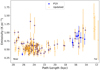 |
Fig. 1 Background emissivity (K pc−1) as a function of path length (kpc) from the considered HII region to the far boundary of the Galaxy. The P19 data are indicated in blue and the updated catalog data are shown in smaller orange dots. The error bars include propagation of the brightness temperature error and the distance error. The x-axis is reversed with respect to path length; short path lengths are on the right and long path lengths on the left. |
4 Method
In this section, we discuss the different steps undertaken to simulate emissivities, and the comparison to the catalog. We use the HAMMURABI code (Waelkens et al. 2009) to simulate the emissivity in the direction of the different HII regions. For this effort we use three GMF models that we discuss briefly in Sect. 4.1, and in addition to that we use the GALPROP1 code (Strong et al. 2009) to simulate the CRE density in the Milky Way, as discussed in Sect. 4.2.
4.1 Galactic magnetic field models
In this work we simulated emissivities by using three different GMF models, and we compared these to the observed emissivities in the catalog. Table 1 contains the general components of the GMF models. The GMF models we use are presented in Planck Collaboration Int. XLII (2016) as the JF12b, Sun10b, and J13b models. In Planck Collaboration Int. XLII (2016) the parameters for these GMF models are adjusted to match the Planck data using a common CRE model. These models are based on the threemodels in Jansson & Farrar (2012a,b), Sun & Reich (2010), and Jaffe et al. (2013), respectively. More detailed information on the GMF model parameters and their determination can be found in Planck Collaboration Int. XLII (2016).
The parameter values for the models have been downloaded from the HAMMURABI sourceforge page2. Some changes were made to the parameter files because of the nature of the setup used in Planck Collaboration Int. XLII (2016), where the Galactic plane in the nearest 2 kpc to the Sun is simulated with higher resolution than the rest of the plane. More specifically we made use of the RG2 parameter files and have adapted them such that all parts of the plane (min_Radius = 0) were integrated.
Galactic magnetic field models.
4.2 Cosmic ray electron models
The GALPROP code (Strong et al. 2009) is developed for the propagation of relativistic charged particles and to simulate diffuse emission that is produced during that propagation. In this work we do not make use of the latter function, but only use GALPROP to calculate a CR density in the Milky Way. This happened in a self-consistent way using the magnetic field model that was employed to calculate the resulting synchrotron emissivity. The GALPROP code uses a configuration file (GALDEF), which specifies source distribution and boundary conditions for the different CR species, to solve the transport equation. The code includes processes such as convection and Galactic wind, diffusive reacceleration, energy loss, and radioactive decay. It is important to note that diffusion is treated isotropically in this code. For consistency with Planck Collaboration Int. XLII (2016) we used the GALDEF z10LMPDE, based on Orlando & Strong (2013). This specific model is the result of a significant body of work of the references therein to develop a model for the spatial and spectral distribution of CR leptons. This model has updated scale heights for the leptons and updated magnetic field parameters, and its spectrum is specifically adjusted to fit the Fermi direct measurements of electrons and positrons as well as diffuse gamma-ray emission. A further improvement gives a better fit to the distribution of synchrotron emission in Galactic longitude and latitude. Further details can be found in the papers mentioned above.
For completion we also discuss the results when using a different GALDEF, to wit, the 71xvarh7S model (Abdo et al. 2010), which is based on a different distribution of CR sources, particularly in the outer Galaxy. The GALDEF was run both in two-dimensional and three-dimensional mode. No significant difference between the runs was detected for any model. The three-dimensional runs are presented in this paper.
4.3 Modeling the emissivities behind the HII regions
We use HAMMURABI (Waelkens et al. 2009) to simulate the synchrotron intensities along specific lines of sight in the Milky Way. To simulate this tracer we need to provide HAMMURABI with a CR density and GMF models as discussed above.
For each HII region the synchrotron intensity was calculated for two parts of the LOS: one intensity integrated over the path from the observer to the HII region (TF) and the other integrated over the path between the Sun and the edge of the Milky Way (TT). Subtracting the former from the latter a value for the intensity integrated over the path between the HII region and the Milky way edge was determined, this is the background simulated measurement. With simple trigonometric calculations and the assumption of a distance from the Sun to the Galactic center of 8.5 kpc and a Galactic radius of 20 kpc, the length of the path between the HII region and the edge of the Milky Way was calculated. Dividing the synchrotron intensity by its companion path length, the synchrotron emissivity for a LOS was computed.
5 Results
In this section, we discuss the distribution of the catalog emissivities compared to the simulated emissivities for three different GMF models and two different CRE models.
Figure 2 shows the averaged emissivity as simulated with the different GMF models, plotted without any extra type of normalization. In P19 we applied an arbitrary scaling to these emissivities to match them with the data owing to an oversimplified CR distribution model. However, when using GALPROP to simulate a realistic CR density such a normalization is not needed.
5.1 Emissivities from observational catalog
First we discuss the catalog data, from which the trend of the data is clearly shown. At the longer path lengths of 28 kpc the data points start with a downward trend, from emissivities of 0.7 K pc−1 down to 0.5 K pc−1 at 26 kpc. This suggests an enhanced contribution of emissivity to HII regions with path lengths between 28 and 26 kpc.
The distribution between 26 and 22 kpc seems to rise and fall again, however we infer that this is a consequence of the sporadic sampling of HII regions for these bins and the fact that HII regions at different longitudes can have the same path lengths. The distribution in this path length region is consistent with a flat trend.
At path lengths below 20 kpc an upward trend starts and around path lengths of 12 kpc a peak of 1.2 K pc−1 is reached. This confirms the results of P19, where we conclude a diminished emissivity in the region around the Galactic center must exist, and/or a high emissivity contribution to the HII regions at the far side of the Galaxy at distances larger than a few kiloparsec from the Galactic center.
The error margin for the HII regions at the short path lengths is relatively large. The assumption of a 50% error for the far HII regions (those that were without a given error in literature) influences this. In addition we notice an increase in the relative error for larger distances, we surmise this is due to the growing uncertainty of the distance determination and the error on the brightness temperature with growing distance to the HII region.
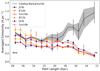 |
Fig. 2 Averaged background emissivity (K pc−1) as a function of the path length (kpc) from the considered HII region to the far boundary of the Galaxy. The catalog data are shown in black, with error margins in gray. This margin consists of the propagated measurement error for the data points in the bin. Also shown is the standard deviation, σ, in the observations as black error bars. The simulated values for two different CRE models are shown for the three different GMF models J13b, JF12b, and Sun10b. The solid line indicates the results for the z10LMPDE CRE model and the dashed line indicates the results for the 71Xvarh7S CRE model. All data – both simulated and catalog values – are averaged into bins with 1 kpc width. The standard deviation for the GMF models is calculated per bin and is plotted. |
5.2 Cosmic ray electron models
In the z10LMPDE CRE model (solid lines) a lower emissivity at shorter path lengths is clearly favored. For the most part, the models show the same large-scale trend. The longer path lengths down to approximately 18 kpc show a flat trend, whereafter the models show a downturn that signifies the lower emissivity contribution in the region behind the Galactic center. This is explained by both a lower GMF strength from the models and a lower CR density from GALPROP in this region of the Galaxy.
For the 71Xvarh7S CRE model (dashed lines) we similarly see clearly that simulated emissivities at longer path lengths are comparable to the catalog emissivities. The JF12b model again shows a deviation from the other models for the longest path lengths, but moving to shorter path lengths it rejoins the other models around 24 kpc. Thereafter the models show a downturn similar to that of the solid lines to finish at a path length of 12 kpc with an emissivity that is too low to be comparable to the catalog emissivities. Again this is due to the lower GMF strength and the CRE density in this region. We include this older model (superseded by z10LMPDE) simply to show that this discrepancy remains for all GMF models even when a different CR source and propagation model is used. We will explore the impact of a larger variety of viable CR models in future work.
Different realizations of the turbulent magnetic field allow for minor variations in the emissivity that is simulated. We investigated these minor variations by running several different realizations and calculating the difference in the output caused by each, and we find an estimated Galactic variance of 3 × 10⁻⁴ K pc−1. Such a small influence of the turbulent field is expected since it is on scales much smaller than what we probe. These fluctuations along the different LOSs are averaged out. A more extensive discussion on the Galactic variance can be found in Planck Collaboration Int. XLII (2016).
In Fig. 3 background emissivities spanning the Galactic plane are plotted for the three different GMF models using the z10LMPDE CRE model. Only one realization of the turbulent magnetic field is shown in this figure. In this view the Sun is located at xy-coordinates (0,−8.5). As was already seen in Fig. 2, the emissivities simulated with the GMF models show a rapid decline in emissivity values with increasing Galactic radii. The structure of the GMF models is clearly visible; the spiral arms are apparent in all three figures and there is a slight asymmetry as a consequence of the pitch angle of the spiral arms.
5.3 Comparison
We want to consider several points in our comparison of the observational and simulation results. Firstly, it shows us that the simulated emissivity values for the z10LMPDE CRE model are only a factor of 2 different in the mean from the observed values, although at longer path lengths the difference is slightly smaller and at short path lengths the difference is slightly larger than this factor of 2. And for the 71Xvarh7S the emissivities at long path lengths are comparable to the catalog values within the error. This is bothsurprising and reassuring considering the uncertainty in the accuracy of both the CRE density and the GMF models. A possible explanation for the factor of 2 could be found in the inaccuracy of the CRE spectrum at the energies that cause the low-frequency synchrotron emission due to the solar modulation. In Fig. 2 of Orlando (2018) it can specifically be seen that at 74 MHz the models are not constrained and could potentially cause the discrepancy. Secondly, the GMF models themselves show results that are comparable to each other. We consider this reasonable in light of the GMF parameter fit done in Planck Collaboration Int. XLII (2016). Thirdly, the trends in the observations and simulations are partially compatible. In the path length range from 28 to 18 kpc the relative flat distribution is reasonably well matched, but beyond 18 kpc the observational trend rises steeply upward, leaving the simulated trend behind.
6 Discussion
In this section we discuss different explanations for two general scenarios concerning the upturn in observational emissivity at short path lengths:
- 1.
The upturn is real.
- 2.
The upturn is not real.
If the upturn is real the models are missing an essential piece of information. If it is not real it is an artifact of wrongly determined HII region emissivities, which can have several sources. Below we discuss several arguments that favor either scenario.
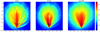 |
Fig. 3 Simulated background emissivities (K pc−1) in color scale with accompanying color bar, calculated for an evenly spaced grid of HII regions in the Galactic plane. The axes are in kiloparsec. The Sun is located at (0,−8.5). Overplotted on all models are the observed background emissivities as colored circles. From left to right: three different GMF models. |
6.1 The upturn is real
If the upward trend at short path lengths is real, this shows that the models underestimate the synchrotron emissivity in the far outer region and/or overestimate the emissivity in the inner region of the Milky Way. This does not subvert the current models nor the tracers used to constrain these models. The discrepancy with current GMF models can simply be explained by the fact that this tracer probes different regions of the Milky Way than other tracers (i.e., the far Galaxy behind the Galactic center). Therefore this discrepancy indicates the need for an extra component in either the CRE density or GMF models; this component results in an enhancement of emissivity in the outer region or a paucity of emissivity in the inner region.
If we consider any change in the emissivity in one region, we have to reflect on the effect it has on the measurements. Any change affects the background measurements for an HII region whose LOS intersects with it. Nevertheless the change in emissivity does not translate into the same change for all such HII regions. Any enhancement in the outer Galaxy changes the emissivities for HII regions with shorter path lengths relatively more than for regions with longer path lengths. This is explained by the higher fraction of their path length that runs through this enhanced region. In this solution it is plausible that the emissivity keeps increasing with decreasing path length if the fraction of enhanced emission keeps increasing with decreasing path length. This could allow for the determination of a lower limit for the distance to this enhanced emission because it has to start behind the HII region that is the farthest away, otherwise the upward trend would have stopped. For our observational data this means the enhanced region would have to start beyond a distance of 16 kpc. This statement is only valid for the longitudinal range that is probed by our catalog. Any broader statements encompassing all longitudes will have to wait for future expansion of the catalog.
An enhanced emissivity could be the result of a higher CRE density or higher magnetic field strength (see Eq. (1)), but could also be the result of a more intermittent magnetic field. As emissivity depends on B , a more clumped magnetic field emits more synchrotron emission than a uniform magnetic field of the same average strength. Therefore, our data might be explained by an increasingly intermittent magnetic field in the outer Galaxy. Intermittent magnetic fields are indeed expected (Seta et al. 2018). However, the intermittency would have to be stronger in the outer Galaxy than in the inner region. We are not aware of any observational or theoretical evidence for this. In addition, enhanced emissivity may also occur if the CRE density and magnetic field are positively correlated, as discussed in Beck et al. (2003). For this correlation to have any effect on the observations it has to be stronger in the outer regions of the Galaxy, similar to the intermittency. For this alternative, we are not aware of observational or theoretical evidence either.
Because we used background emissivity measurements any paucity in the inner region does not affect emissivities of HII regions that are beyond this inner region. In P19 we briefly discuss this region of diminished emissivity in the Galactic center region and put forward that it may be due to outflows and x-shaped magnetic fields in this area. Outflows are also described in Carretti et al. (2013), and even if the size of the region they consider is an order of magnitude smaller than ours we still consider this option a possibility.
6.1.1 Toy models: inner underdensity
In an effort to substantiate our hypotheses of an outer region with an enhanced emissivity contribution and an inner region with a diminished emissivity contribution we created four simple toy models that exemplify this. To implement a toy emissivity model, we hold the CRE component constant over the Milky Way and vary the GMF strength for three models and the pitch angle for one. For the purposes of these simple toy models, varying the GMF strength alone has the same effect on the synchrotron emission as varying the CRE density. All the details of the different models can be found together in Table 2. For all models, the outer 1 kpc is devoid of emissivity. This was chosen for numerical reasons near the boundary.
It is important to mention that models 1, 3, and 4 have a spiral structure due to the non-zero pitch angle. Model 2 however has a circular orientation of the magnetic field lines owing to its pitch angle of zero degrees. The inner region for all the models is a circular region with a radius of 8 kpc for models 1, 2, and 4, and a radius of 3 kpc for model 3. Models 1, 2, and 3 have an inner circular region devoid of magnetic field strength, whereas model 4 has half that of the outer region.
Owing to the arbitrary values of the magnetic field and the constant CRE density model, these toy models need to be normalized to the catalog data before we can start the comparison. We do this by employing a least-squares fit of the models to the catalog data. The result is shown in Fig. 4.
The relative ratios of the models disappear as a result of normalization. Therefore, we confine ourselves to general statements about trends and features.
The most remarkable feature of the toy models is the upward trend, which is not an artifact of normalization. Even though the constant CRE density and the limited magnetic field components used combine into a physically unlikely scenario, the contribution it provides to the shortest path length shows a striking resemblance to the observational trend. This leads us to our most important conclusion, that either a diminished emissivity in the inner Galactic region or an enhanced emissivity in the outer region – or likely a combination of both – can emulate the steepness of the observational trend at the shortening path lengths.
We can further discuss the different models by steepness of trend. Models 1 and 2 show the steepest of the trends and the emissivity picked up for the longer path lengths is lowest. This makes sense because these path lengths, at least partially, run through the “empty” region in the center and no emissivity is contributed in this part of the path length. The shorter path lengths are influenced least by the central region, which is a general remark for all four models. Model 4 is less steep than models 1 and 2. Its central region has an emissivity contribution, so the longer path lengths pickup more emissivity and this contributes to a flatter distribution. With the smallest radius of the inner region, model 3 has the flattest distribution. In this case, relatively more emissivity is picked up on the longer path lengths. We can conclude that the size of the inner region is correlated with the flattening of the distribution,and a smaller inner region (model 3) likely does not show the steepness needed to explain the trend in the observations.
Finally, the influence of a pitch angle is clear: for model 2 (pitch angle of zero degrees) the emissivity distribution is much smoother and does not show the dips at path lengths of 15 kpc and 22 kpc. This feature is also seen in the observational distribution. We conclude that for our uneven sampling a non-zero pitch angle is a prerequisite for any GMF model.
The impact of the pitch angle is much clearer in Fig. 5. This can be seen in the results for model 2, which shows a symmetric emissivity distribution, where the rest of these models show a distinct asymmetry. It is this asymmetry that is unevenly sampled by our HII catalog that leads to the peaks and troughs in the curves in Fig. 4
The toy models show other clear and understandable internal differences. Model 1 in Fig. 5 shows strong emissivities in roughly the anti-center direction and in the first quarter beyond the inner region of 8 kpc that has no emissivity contribution. In this inner region the emissivity declines for HII regions that are closer to the observer because of the increasing ratio of empty space over the path length. Model 3 has a smaller inner region, as a consequence of this we see in Fig. 5 that more background emissivity is picked up for the HII regions in this center area. This is explained by a larger region in which synchrotron emission can be produced. Model 4 has an increased magnetic field strength in the inner 8 kpc, which can be clearly seen by the increased emissivity in this region. However, in our toy models a higher inner magnetic field strength causes a smaller increase in the emissivity in this region than in a model that has a smaller inner empty region.
Toy models with an underdensity in the inner Galaxy.
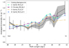 |
Fig. 4 Background emissivity (K pc−1) as a function of path length (kpc) from the considered HII region to the far boundary of the Galaxy. The catalog data are shown in black and the error margin in gray; the four different toy models are shown as follows: model 1 (green triangles), model 2 (purple dots), model 3 (yellow stars), and model 4 (blue squares). |
6.1.2 Toy models: annuli
To constrain properties of the enhanced emissivity in the outer region of the Milky Way we use an additional set of toy models. The parameters for these models are described in Table 3 and the results are plotted in Fig. 6. These models are annuli with different inner and outer radii and are all centered on the Galactic center. Model 5 has an inner radius of 6 kpc and an outer radius of 10 kpc. Models 6 through 8 all have an inner radius of 3 kpc and increasing outer radii of 5, 7, and 10 kpc. For all these models the area that is covered by the annulus has a magnetic field strength of 1.0 μG and the area that is not covered by the annulus a magnetic field strength of zero. All models have a pitch angle of −12.0 degrees. Like for the other set of toy models, the CRE component is kept constant over the entire Milky Way, and a normalization of these toy models was performed.
Depending on the width and location of the annulus many or few HII regions pick up emissivity. It is clear at the right-hand side of Fig. 6 that the absence of emissivity in the outer region of the Galaxy impacts the HII regions with short path lengths. All the models show a decline or even absence of emissivity there. This cannot be reconciled with the upward trend of the observations. The impact of the size of the annulus is also clear, specifically for models 6–8, which show an increasingly flattening trend with increasing annulus size. However the absence of emissivity behind the farthest HII regions will never allow these models to display a trend that is comparable to the observations. From this we are forced to conclude that any model used to describe the observations has a need for emissivity beyond a 10 kpc Galactic radius in the far outer Galaxy.
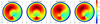 |
Fig. 5 Simulated background emissivities calculated for an evenly spaced grid of HII regions in the Galactic plane. The axes are in kiloparsec; the Sun is located at (0,−8.5). From left to right: toy model 1, toy model 2, toy model 3, and toy model 4. For clarity the radii for the inner region are plotted in black. No normalization of the values has been performed. |
Toy models with an underdensity in the inner and outer Galaxy.
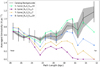 |
Fig. 6 Background emissivity (K pc−1) as a function of path length (kpc) from the considered HII region to the far boundary of the Galaxy. The P19 data are shown in black and the error margin in gray. The four different toy models are shown: model 5 (green triangles), model 6 (purple dots), model 7 (yellow stars), and model 8 (blue squares). |
6.2 The upturn is not real
If the upward trend at short path lengths is not real, then either the radius of the Milky Way is wrongly chosen or there is a problem with the distance determination for HII regions. This section discusses these options in detail.
To calculate the path lengths for the background emissivities, a radius for the Galaxy has to be assumed. In previous work and this work we assume that this radius is 20 kpc. Assuming a larger radius adjusts the emissivity values in the catalog in a downward fashion, although the trend remains the same. A smaller radius drives the emissivity values up and also does not change the trend, additionally it unnecessarily confines the region within which synchrotron emission could be produced. Considering the incompatible trends of the observations and the models, we looked into changing this variable to an arbitrary larger value of 30 kpc. We found that this procedure does not change the trend of our observations.
The determination of kinematic distances of HII regions has the inherent issue of ambiguity: the region is either located at the near or far distance solution. As discussed in Sect. 3.1, observations of other tracers can break this degeneracy. However, if we assume that this method does not always work, there might be HII regions that are currently categorized in the far distance that are at the near distance. In our sample, a by-eye investigation reveals that roughly nine HII regions withpath lengths smaller than 20 kpc would have to move to counteract the upward trend. This would diminish the support for the rising trend on the right-hand side of Fig. 1 and would bring the observed trend closer to the models. Taking this line of reasoning one step further, all but two HII regions with path lengths shorter than 20 kpc would have to move to make the catalog data compatible with the simulated emissivities in Fig. 2. Unfortunately, this leaves most of the short path length regime unprobed, and no informative comparison can be made between the catalog and simulated emissivities. In addition, for some of these HII regions the distances were determined accurately with a different method, therefore this upward trend will not disappear.
Although it seems unlikely that far distances to all HII regions in our catalog are wrongly determined, we need to take into account a bias that may increase its probability. As stated in N06, the detection of these HII regions is not due to their own emission, but through the emission that is being blocked by them. HII regions that are blocking a column of lower synchrotron emissivity have a smaller chance of being detected in this way. This might explain why, at large distances from the observer, the only regions detected have emissivity values that appear to be enhanced. We note that this detection bias does not make the existing data at short path lengths disappear. Furthermore, accuracy of HII region distance determination is beyond the scope of this paper.
7 Conclusions
Summarizing our main conclusions, we state that our observations imply either that there is a problem with the distance determination of part of the distant HII regions, or that there is a change in the emissivity contribution in either the inner region (paucity) or the outer region (enhancement) of the Galaxy.
Assuming that the latter options are more likely, a region with a diminished emissivity contribution is likely located in the inner 8 kpc. This paucity can be caused by an outflow of CREs and/or a lack of perpendicular (to the LOS) magnetic field lines in this region. Conversely, a region for an emissivity enhancement has to be at least 16 kpc away from the sun in the Galactic center direction. This region has to spread out over a longitude range that is probed by our catalog (–43° < ℓ < 25°). The enhancement of synchrotron emissivity can be caused by (1) extra CREs, perhaps a single isolated source; (2) higher magnetic field strength; (3) intermittency of the magnetic field; and (4) positive correlation between CRE density and the GMF in the region behind the Galactic center.
Acknowledgements
I.M.P. would like to acknowledge funding from the Netherlands Research School for Astronomy (NOVA). Carmelo Evoli, Anvar Shukurov and Elena Orlando are thanked for fruitful discussions on different parts of this work. M.H. acknowledges funding from the European Research Council (ERC) under the European Union’s Horizon 2020 research and innovation programme (grant agreement No 772663). This research made extensive use of NumPy (van der Walt et al. 2011); IPython (Perez & Granger 2007) and matplotlib (Hunter 2007). The authors would like to thank the ADS abstract service. The authors would like to thank the referee for suggestions that have improved this paper.
Appendix A Additional table
Complete and updated catalog of HII regions detected in absorption.
References
- Abdo, A. A., Ackermann, M., Ajello, M., et al. 2010, ApJ, 710, 133 [NASA ADS] [CrossRef] [Google Scholar]
- Anderson, L. D., Bania, T. M., Balser, D. S., et al. 2014, ApJS, 212, 1 [NASA ADS] [CrossRef] [Google Scholar]
- Anderson, L. D., Wenger, T. V., Armentrout, W. P., Balser, D. S., & Bania, T. M. 2019, ApJ, 871, 145 [NASA ADS] [CrossRef] [Google Scholar]
- Azcárate, I. I. A. d. R., Cersósimo, J. I. A. d. R., & Colomb, F. I. A. d. R. 1990, Rev. Mex. Astron. Astrofis., 20, 23 [NASA ADS] [Google Scholar]
- Balser, D. S., Wenger, T. V., Anderson, L. D., & Bania, T. M. 2015, ApJ., 806, 199 [NASA ADS] [CrossRef] [Google Scholar]
- Beck, R., Shukurov, A., Sokoloff, D., & Wielebinski, R. 2003, A&A, 411, 99 [NASA ADS] [CrossRef] [EDP Sciences] [Google Scholar]
- Carretti, E., Crocker, R. M., Staveley-Smith, L., et al. 2013, Nature, 493, 66 [NASA ADS] [CrossRef] [PubMed] [Google Scholar]
- Fauvet, L., Macías-Pérez, J. F., Aumont, J., et al. 2011, A&A, 526, A145 [NASA ADS] [CrossRef] [EDP Sciences] [Google Scholar]
- Ferrière, K. M. 2001, Rev. Mod. Phys., 73, 1031 [NASA ADS] [CrossRef] [Google Scholar]
- Hall, J. S. 1949, Science, 109, 166 [NASA ADS] [CrossRef] [Google Scholar]
- Han, J. L. 2017, ARA&A, 55, 111 [NASA ADS] [CrossRef] [Google Scholar]
- Haverkorn, M. 2015, Astrophys. Space Sci. Lib., 407, 483 [NASA ADS] [CrossRef] [Google Scholar]
- Heiles, C., & Haverkorn, M. 2012, Space Sci. Rev., 166, 293 [NASA ADS] [CrossRef] [EDP Sciences] [Google Scholar]
- Hiltner, W. A. 1949a, ApJ, 109, 471 [NASA ADS] [CrossRef] [Google Scholar]
- Hiltner, W. A. 1949b, Science, 109, 165 [NASA ADS] [CrossRef] [Google Scholar]
- Hindson, L., Johnston-Hollitt, M., Hurley-Walker, N., et al. 2016, PASA, 33, e020 [NASA ADS] [CrossRef] [Google Scholar]
- Hunter, J. D. 2007, Comput. Sci. Eng., 9, 90 [NASA ADS] [CrossRef] [Google Scholar]
- Jaffe, T. R. 2019, Galaxies, 7, 52 [NASA ADS] [CrossRef] [Google Scholar]
- Jaffe, T. R., Ferrière, K. M., Banday, A. J., et al. 2013, MNRAS, 431, 683 [NASA ADS] [CrossRef] [Google Scholar]
- Jansson, R., & Farrar, G. R. 2012a, ApJ, 757, 14 [NASA ADS] [CrossRef] [Google Scholar]
- Jansson, R., & Farrar, G. R. 2012b, ApJ, 761, L11 [NASA ADS] [CrossRef] [Google Scholar]
- Jones, B., & Finlay, E. 1974, Aust. J. Phys., 27, 687 [NASA ADS] [CrossRef] [Google Scholar]
- Kassim, N. E. 1990, Lect. Notes Phys., 362, 144 [NASA ADS] [CrossRef] [Google Scholar]
- Nord, M. E., Henning, P. A., Rand, R. J., Lazio, T. J. W., & Kassim, N. E. 2006, AJ, 132, 242 [NASA ADS] [CrossRef] [Google Scholar]
- Noutsos, A. 2012, Space Sci. Rev., 166, 307 [NASA ADS] [CrossRef] [Google Scholar]
- Odegard, N. 1986, ApJ, 301, 813 [NASA ADS] [CrossRef] [Google Scholar]
- Orlando, E. 2018, MNRAS, 2742, 2724 [NASA ADS] [CrossRef] [Google Scholar]
- Orlando, E., & Strong, A. 2013, MNRAS, 436, 2127 [NASA ADS] [CrossRef] [Google Scholar]
- Page, L., Hinshaw, G., Komatsu, E., et al. 2007, ApJS, 170, 335 [NASA ADS] [CrossRef] [Google Scholar]
- Paladini, R., Burigana, C., Davies, R. D., et al. 2003, A&A, 397, 213 [NASA ADS] [CrossRef] [EDP Sciences] [Google Scholar]
- Perez, F., & Granger, B. E. 2007, Comput. Sci. Eng., 9, 21 [Google Scholar]
- Planck Collaboration XXV. 2016, A&A, 594, A25 [NASA ADS] [CrossRef] [EDP Sciences] [Google Scholar]
- Planck Collaboration Int. XLII. 2016, A&A, 596, A103 [NASA ADS] [CrossRef] [EDP Sciences] [Google Scholar]
- Polderman, I. M., Haverkorn, M., Jaffe, T. R., & Alves, M. I. R. 2019, A&A, 621, A127 [NASA ADS] [CrossRef] [EDP Sciences] [Google Scholar]
- Quireza, C., Rood, R. T., Balser, D. S., & Bania, T. M. 2006, ApJS, 165, 338 [NASA ADS] [CrossRef] [Google Scholar]
- Reid, M. J., Menten, K. M., Brunthaler, A., et al. 2014, ApJ, 783, 130 [Google Scholar]
- Roger, R. S., Costain, C. H., Landecker, T. L., & Swerdlyk, C. M. 1999, A&A, 19, 7 [Google Scholar]
- Seta, A., Shukurov, A., Wood, T. S., Bushby, P. J., & Snodin, A. P. 2018, MNRAS, 473, 4544 [NASA ADS] [CrossRef] [Google Scholar]
- Shukurov, A., Rodrigues, L. F. S., Bushby, P. J., Hollins, J., & Rachen, J. P. 2019, A&A, 623, A113 [NASA ADS] [CrossRef] [EDP Sciences] [Google Scholar]
- Strong, A. W., Moskalenko, I. V., Porter, T. A., et al. 2009, ArXiv e-prints [arXiv:0907.0559] [Google Scholar]
- Su, H., Hurley-Walker, N., Jackson, C. A., et al. 2016, MNRAS, 13, 1 [Google Scholar]
- Su, H., Macquart, J. P., Hurley-Walker, N., et al. 2018, MNRAS, 479, 4041 [NASA ADS] [CrossRef] [Google Scholar]
- Sun, X. H. & Reich, W. 2010, Res. Astron. Astrophys., 10, 1287 [NASA ADS] [CrossRef] [Google Scholar]
- Tinyakov, P. G., & Tkachev, I. I. 2002, Astropart. Phys., 18, 165 [NASA ADS] [CrossRef] [Google Scholar]
- van der Walt, S., Colbert, S. C., & Varoquaux, G. 2011, Comput. Sci. Eng., 13, 22 [Google Scholar]
- Van Eck, C. L., Brown, J. C., Stil, J. M., et al. 2011, ApJ, 728, 97 [NASA ADS] [CrossRef] [Google Scholar]
- Waelkens, A., Jaffe, T., Reinecke, M., Kitaura, F. S., & Enßlin, T. A. 2009, A&A, 495, 697 [NASA ADS] [CrossRef] [EDP Sciences] [Google Scholar]
- Wielebinski, R., & Beck, R., eds. 2005, Cosmic Magnetic Field, Lect. Notes Phys. (Berlin: Springer Verlag), 664 [Google Scholar]
All Tables
All Figures
|
Fig. 1 Background emissivity (K pc−1) as a function of path length (kpc) from the considered HII region to the far boundary of the Galaxy. The P19 data are indicated in blue and the updated catalog data are shown in smaller orange dots. The error bars include propagation of the brightness temperature error and the distance error. The x-axis is reversed with respect to path length; short path lengths are on the right and long path lengths on the left. |
| In the text | |
|
Fig. 2 Averaged background emissivity (K pc−1) as a function of the path length (kpc) from the considered HII region to the far boundary of the Galaxy. The catalog data are shown in black, with error margins in gray. This margin consists of the propagated measurement error for the data points in the bin. Also shown is the standard deviation, σ, in the observations as black error bars. The simulated values for two different CRE models are shown for the three different GMF models J13b, JF12b, and Sun10b. The solid line indicates the results for the z10LMPDE CRE model and the dashed line indicates the results for the 71Xvarh7S CRE model. All data – both simulated and catalog values – are averaged into bins with 1 kpc width. The standard deviation for the GMF models is calculated per bin and is plotted. |
| In the text | |
|
Fig. 3 Simulated background emissivities (K pc−1) in color scale with accompanying color bar, calculated for an evenly spaced grid of HII regions in the Galactic plane. The axes are in kiloparsec. The Sun is located at (0,−8.5). Overplotted on all models are the observed background emissivities as colored circles. From left to right: three different GMF models. |
| In the text | |
|
Fig. 4 Background emissivity (K pc−1) as a function of path length (kpc) from the considered HII region to the far boundary of the Galaxy. The catalog data are shown in black and the error margin in gray; the four different toy models are shown as follows: model 1 (green triangles), model 2 (purple dots), model 3 (yellow stars), and model 4 (blue squares). |
| In the text | |
|
Fig. 5 Simulated background emissivities calculated for an evenly spaced grid of HII regions in the Galactic plane. The axes are in kiloparsec; the Sun is located at (0,−8.5). From left to right: toy model 1, toy model 2, toy model 3, and toy model 4. For clarity the radii for the inner region are plotted in black. No normalization of the values has been performed. |
| In the text | |
|
Fig. 6 Background emissivity (K pc−1) as a function of path length (kpc) from the considered HII region to the far boundary of the Galaxy. The P19 data are shown in black and the error margin in gray. The four different toy models are shown: model 5 (green triangles), model 6 (purple dots), model 7 (yellow stars), and model 8 (blue squares). |
| In the text | |
Current usage metrics show cumulative count of Article Views (full-text article views including HTML views, PDF and ePub downloads, according to the available data) and Abstracts Views on Vision4Press platform.
Data correspond to usage on the plateform after 2015. The current usage metrics is available 48-96 hours after online publication and is updated daily on week days.
Initial download of the metrics may take a while.