© ESO 2020

1. Introduction

Radio pulsars are known for their stable rotational period. Nevertheless, several pulsars exhibit sudden and sporadic spin-up events of small amplitude, known as glitches (Espinoza et al. 2011). Since the pioneering work of Baym et al. (1969), several models have been proposed to describe glitches by formally dividing the spinning neutron star into two parts: a normal component, corotating with the observed beamed radiation of magnetospheric origin, and a superfluid neutron component (Haskell & Melatos 2015). A difference of angular velocity may develop between the two components (constituting a reservoir of angular momentum) thanks to the pinning of the superfluid vortices to impurities of the crustal lattice (Anderson & Itoh 1975) or to the quantised flux tubes of magnetic field permeating the outer core (Gügercinoğlu & Alpar 2014). Following this paradigm, several models were employed to study glitching pulsars, yielding indirect constraints on the neutron star structural properties through observations (Datta & Alpar 1993; Link et al. 1999; Andersson et al. 2012; Chamel 2013; Newton et al. 2015; Ho et al. 2015; Pizzochero et al. 2017; Montoli et al. 2020).

The possibility to test our understanding of the glitch mechanism is hindered by the difficulty of observing glitches in the act. In fact, glitch rises are generally not resolved, due to intrinsic noise in the time of arrival of single pulsations. Moreover, in spite of the fact that the Vela pulsar has been monitored for fifty years, only in a couple of notable events has it been possible to put an upper limit of 40 s on the timescale of the glitch spin-up (Dodson et al. 2002, 2007). Only recently, with the observation of a glitch on 12 December 2016, did it become possible to measure the time of arrival of single pulses during the glitch with unprecedented precision, and thus to obtain some information on the first seconds after the event (Palfreyman et al. 2018). In particular, a new strong upper limit of 12.6 s on the timescale of the glitch spin-up has been determined by Ashton et al. (2019). This kind of observation opens a new window for theoretical speculations. In fact, complex behaviour during the spin-up and the first minute of the post-glitch relaxation has been predicted in simulations based on hydrodynamical models of the neutron star internal structure, when more than just two rigid components are considered (Haskell et al. 2012; Haskell & Antonopoulou 2014; Antonelli & Pizzochero 2017; Graber et al. 2018): when the superfluid component is allowed to sustain non-uniform rotation, different regions may experience different friction, and hence recouple to the observable normal component on different timescales, giving different glitch shapes.

In particular, depending on the strength of the couplings and on the initial conditions for the relative motion between the various components, a glitch overshoot a transient interval in which the observable component spins at a higher rate than the post-glitch equilibrium value, obtained by emptying the whole angular momentum stored into the superfluid reservoir (Antonelli & Pizzochero 2017) is observed in such models.

Two recent studies have already used the data from the 2016 glitch: in Graber et al. (2018), the drag between the charged crust and the crustal and core superfluids has been constrained; in Ashton et al. (2019), different phenomenological models have been compared to the timing results, obtaining the best current limits on the glitch rise timescale. Both studies also confirmed the presence of an overshoot.

In this article, we first give a simple quantitative result for the onset of a glitch overshoot, by employing a three-rigid-component model for the glitch dynamics (which is the minimal model capable of reproducing an overshoot). We then use the model to fit the 2016 glitch of the Vela pulsar. The advantage of the present treatment is that it provides an analytical form for the timing residuals, which is directly related to physical parameters of the neutron star. Indeed, in addition to determining the rise and decay timescales of the overshoot, the fit results make it possible to derive some physical properties of the three components, such as the moment of inertia fractions and the drag parameters between the two superfluid components and the normal one.

2. Three-component model

Generalising the approach of Baym et al. (1969), the pulsar is described by means of three rigidly rotating components. We consider two neutron superfluid components (labelled with 1, 2 subscripts), that exchange angular momentum with a normal component p on timescales τ_1, 2. The p-component is interpreted as all the charged particles coupled to the observable magnetosphere on timescales shorter than τ₁ and τ₂, while we do not need to specify what the two superfluid components are: in fact, the equations we are going to write are completely general, as they derive from conservation of angular momentum and the only assumption of rigid rotation of the three components. Physically, however, they could represent the P-wave superfluid in the core, and the S-wave one the crust, as the physical conditions of these regions are completely different. We thus employ a set of three equations, one for the conservation of angular momentum, and two representing the interaction between the normal component and each of the two superfluid components:

$$\begin{array}{c}\hfill \begin{array}{cc}\hfill {\dot{\mathrm{\Omega }}}_p& =-\frac{1}{x_p}(x_1{\dot{\mathrm{\Omega }}}_1+x_2{\dot{\mathrm{\Omega }}}_2+|{\dot{\mathrm{\Omega }}}_{\infty }|)\hfill \\ \hfill {\dot{\mathrm{\Omega }}}_1& =-x_p\frac{{\mathrm{\Omega }}_1-{\mathrm{\Omega }}_p}{{\tau }_1}=-x_p\frac{{\mathrm{\Omega }}_{1p}}{{\tau }_1}\hfill \\ \hfill {\dot{\mathrm{\Omega }}}_2& =-x_p\frac{{\mathrm{\Omega }}_2-{\mathrm{\Omega }}_p}{{\tau }_2}=-x_p\frac{{\mathrm{\Omega }}_{1p}}{{\tau }_1},\hfill \end{array}\end{array}$$(1)

where Ω_ip = Ω_i − Ω_p (i = 1,  2) are the lags, and where x_i = I_i/I (i = 1,  2,  p) are the ratios of the partial moment of inertia I_i of the i-component with respect to the total one I = I₁ + I₂ + I_p, so that x₁ + x₂ + x_p = 1. The quantity $|{\dot{\mathrm{\Omega }}}_{\infty }|$ sets the intensity of the external braking torque (for Vela ${\dot{\mathrm{\Omega }}}_{\infty }\approx -9.78\times {10}^{-11}$ rad s⁻², but its precise value is unimportant in the following analysis). Equation (1) is valid without superfluid entrainment: this is discussed in a dedicated section.

We note that a three-component model was also introduced in Graber et al. (2018), but with a differential rotation associated to the reservoir: this was necessary to study the density-dependent drag parameters, but it requires a numerical integration of the dynamical equations. The model in Eq. (1), to which the equations in Graber et al. (2018) reduce when imposing rigid rotation and constant drag, is the simplest analytical treatment that can reproduce an overshoot, making it possible to directly derive the average properties of the superfluid components (fractional moment of inertia and average drag).

For a real pulsar, we expect the two timescales τ_1, 2 to be complicated functions of the instantaneous angular velocity lags Ω_ip = Ω_i − Ω_p and also to depend on the past history of the vortex configuration and internal stresses. In a model with rigid components, these timescales define the strength of the vortex-mediated mutual friction, which is responsible for the angular momentum exchange, suitably averaged over the region of interest. To better compare with Graber et al. (2018), the timescales τ_i can be connected to the large-scale hydrodynamic mutual friction coefficients ℬ_i. In turn, these are related to the dimensionless drag parameters ℛ_i (which are the results of theoretical calculations) by the relation ${\mathcal{B}}_i={\mathcal{R}}_i/(1+{\mathcal{R}}_i^2)$, see, for example, Andersson et al. (2006). The dynamical equations for rigidly rotating superfluids in the presence of mutual friction are (see e.g. Haskell & Melatos 2015):

$$\begin{array}{c}\hfill {\dot{\mathrm{\Omega }}}_i=-2{\mathrm{\Omega }}_i{\mathcal{B}}_i({\mathrm{\Omega }}_i-{\mathrm{\Omega }}_p)\simeq -2{\mathrm{\Omega }}_p(0){\mathcal{B}}_i({\mathrm{\Omega }}_i-{\mathrm{\Omega }}_p)(i=1,2),\end{array}$$(2)

where we approximated Ω₁ = Ω₂ = Ω_p(0) in the prefactor, since the lags between the superfluids and the normal component are always orders of magnitude smaller than the angular velocity of the normal component. Comparing Eqs. (1) and (2), we can write the (approximate) relation:

$$\begin{array}{c}\hfill {\mathcal{B}}_i=\frac{x_p}{2{\mathrm{\Omega }}_p(0){\tau }_i}(i=1,2).\end{array}$$(3)

In the following, we take a nominal value Ω_p(0) = 70.29 rad s⁻¹ (Dodson et al. 2002).

How to construct realistic models of vortex-mediated mutual friction (i.e. understanding the many-vortex dynamics in neutron stars in the presence of pinning sites) is one of the current challenges of glitch theory. In the present phenomenological description, we assume that, at the glitch time, τ_1, 2 undergo a transition from large “pre-trigger” values to much smaller “post-trigger” values: the nature of the trigger is undetermined, but, according to this simple picture, the vortices change their state of motion, increasing their creep rate, and thus mimicking the onset of a vortex avalanche (Alpar et al. 1984). In fact, if the vortices of the i-component are pinned, or their motion is severely hindered, the timescale τ_i diverges, so that the corresponding Ω_i remains constant regardless of the state of motion of the other components. Therefore, pinning implies the decoupling of that component from the rest of the system, while a sudden recoupling of such a component results in an exchange of angular momentum from the superfluid to the crust, leading to a glitch.

We now study the solutions of the system (1). Since the main goal of the present analysis is to provide the simplest criteria for overshooting glitches, we take τ₁ and τ₂ as constants for t >  0, thus neglecting the repinning process (which may be, nonetheless, important for a complete description of the inter-glitch dynamics): this approximation should hold at least for the overshoot phase.

Firstly, it is useful to rewrite the problem using the lags Ω_ip as variables instead of Ω₁ and Ω₂. This way, the two equations for ${\dot{\mathrm{\Omega }}}_{\mathit{ip}}$ do not depend on Ω_p, and it is possible to solve them independently from the equation for ${\dot{\mathrm{\Omega }}}_p$. To set the unknown initial conditions ${\mathrm{\Omega }}_{ip}^0$, we rely on a physical assumption: we impose component 1 as a “passive” one that does not change its creep rate (i.e. τ₁ is always constant and ${\mathrm{\Omega }}_{1p}^0={\tau }_1|{\dot{\mathrm{\Omega }}}_{\infty }|/x_p$), while component 2 (acting as the reservoir) has a lag ${\mathrm{\Omega }}_{2p}^0=\omega (0)+{\tau }_2|{\dot{\mathrm{\Omega }}}_{\infty }|/x_p$. The positive quantity ω(0) is the excess lag with respect to the asymptotic post-glitch steady-state lag, which has been accumulated before the triggering event.

The angular velocity of the normal component for t >  0 can now be written as ${\mathrm{\Omega }}_p(t)={\mathrm{\Omega }}_p^0+{\dot{\mathrm{\Omega }}}_{\infty }t+\mathrm{\Delta }{\mathrm{\Omega }}_p(t)$, where the difference with respect to the steady-state, $\mathrm{\Delta }{\mathrm{\Omega }}_p(t)={\mathrm{\Omega }}_p(t)-{\mathrm{\Omega }}_p^0-{\dot{\mathrm{\Omega }}}_{\infty }t$, is given by

$$\begin{array}{c}\hfill \mathrm{\Delta }{\mathrm{\Omega }}_p(t)=\mathrm{\Delta }{\mathrm{\Omega }}_p^{\infty }-ϵ\frac{Q+R}{{\tau }_{+}}{e}^{-t/{\tau }_{-}}+ϵ\frac{Q-R}{{\tau }_{-}}{e}^{-t/{\tau }_{+}},\end{array}$$(4)

where $\mathrm{\Delta }{\mathrm{\Omega }}_p^{\infty }=x_2\omega (0)$. In the above expression, the following constants have been defined:

$$\begin{array}{cc}& Q=1-x_1-\beta (1-2x_1-x_2)\hfill \end{array}$$(5)

$$\begin{array}{cc}& R=\sqrt{{[1-x_1+\beta (1-x_2)]}^2-4\beta (1-x_1-x_2)}\hfill \end{array}$$(6)

$$\begin{array}{cc}& ϵ=\frac{x_2{\tau }_1}{2(1-x_1-x_2)R}\omega (0)\hfill \end{array}$$(7)

$$\begin{array}{cc}& {\tau }_{\pm }=\frac{2\beta {\tau }_1}{1-x_1+\beta (1-x_2)\mp R},\hfill \end{array}$$(8)

where β = τ₂/τ₁ is the ratio between the two timescales and τ₊ >  τ₋ >  0.

We note that our solution, Eq. (4), has the same form of one of the phenomenological models studied in Ashton et al. (2019). Here, we make the further step of connecting the coefficients of the two exponentials and the timescales τ₋ and τ₊ to physical parameters of the neutron star, that can thus be inferred after comparison with the data.

It is interesting to point out some properties of the expression in (4). Firstly, we have $\mathrm{\Delta }{\mathrm{\Omega }}_p\to \mathrm{\Delta }{\mathrm{\Omega }}_p^{\infty }$ for t → ∞, which is the glitch amplitude measured at t ≫ τ₊. The glitch amplitude, however, can overcome this asymptotic value at earlier times: the presence of such an overshoot is revealed by the existence of a maximum in ΔΩ_p(t), occurring at time

$$\begin{array}{c}\hfill t_{\max }=\frac{{\tau }_1\beta }{R}ln\left(\frac{Q+R}{Q-R}\right).\end{array}$$(9)

The maximum exists only if the argument of the logarithm is positive, which implies β <  1. In other words, the condition for an overshoot is that the post-glitch timescale τ₂ associated to the “active” component (that in the pre-glitch state was only loosely coupled to the rest of the star) must be smaller than the timescale τ₁ of the “passive” component (that does not change its coupling). From the physical point of view, the overshoot occurs if the “active” superfluid region that stores the angular momentum for the glitch can transfer its excess of angular momentum to the normal component faster than the typical timescale the “passive” superfluid component reacts with. This behaviour can already be seen in Fig. 3 of Graber et al. (2018), and was explicitly noted in Ashton et al. (2019). We confirm this here, by giving it a mathematical foundation.

Following Graber et al. (2018), we now study the time dependence of the time residuals r(t) with respect to the timing model of a uniformly decelerating pulsar:

$$\begin{array}{c}\hfill r(t)=r_0-\frac{1}{{\mathrm{\Omega }}_p(0)}{\displaystyle {\int }_0^t}\mathrm{\Delta }{\mathrm{\Omega }}_p(t^{\prime })\mathrm{d}{\displaystyle t\prime },\end{array}$$(10)

where a constant residual r₀ has been added to account for an offset due to magnetospheric changes. It is easy to see how the condition for the overshoot is translated in terms of the residuals: the glitch presents an overshoot if r(t) is first concave downwards, then upwards, with a flex point at t = t_max. Conversely, a non-overshooting glitch is always concave downwards. In Fig. 1, we show the behaviour of both the angular velocity with respect to the steady state and of the residuals, for β = 0.1 <  1 (overshoot) and for β = 1.1 >  1 (no overshoot).

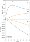Fig. 1. Representation of a glitch with (β = 0.1) and without (β = 1.1) overshoot. The remaining parameters are taken from Table 1. Upper panel: angular velocity with respect to the steady state, ΔΩp(t), lower panel: (shifted) residuals, r(t) − r0. The flex in the residuals for the glitch with overshoot is marked by the intersection with the vertical line at t = tmax.

Looking at the averaged data for the 2016 Vela glitch shown in Fig. 5 of Graber et al. (2018), we deduce that that glitch presents an overshoot, as it shows a positive concavity before reaching steady-state. The first instants of negative concavity are lost, probably due to the extremely fast acceleration of the star and to the magnetospheric change in the pulsar magnetic field (Palfreyman et al. 2018), although a flex can be detected (with difficulty, due to the scale of the figure) in the solid line a few seconds after the beginning of the glitch. The overshoot was also recently confirmed by Ashton et al. (2019).

3. Fit to the 2016 Vela glitch

We now fit expression (10) (which contains seven independent parameters) to the data of the residuals made available by Palfreyman et al. (2018) using a least-squares method. However, some precautions have to be taken. Firstly, although the glitch time t_gl and amplitude $\mathrm{\Delta }{\mathrm{\Omega }}_p^{\infty }$ were already estimated by Palfreyman et al. (2018), here we take them as free parameters, thus allowing for a check of our results. Secondly, as noticed by Palfreyman et al. (2018), soon after a null (missing) pulse at time t₀, a sudden and persistent increase of the timing residuals has been detected in the time interval between t₁ = t₀ + 1.8 s and t₂ = t₀ + 4.4 s (cf. Fig. 2 for the relative positions of these times). This behaviour may correspond to a slow down of the star just before the glitch (Ashton et al. 2019) or to a magnetospheric change in the star (Palfreyman et al. 2018). As we are not able to model this kind of phenomena with the current equations, we simply consider the resulting positive offset in the timing residuals r₀ as a variable for our fit. For the same reason, we have to neglect some of the data after the occurrence of the glitch. During the interval Δt_m = t₂ − t₁, the emitting magnetosphere indeed decoupled from (is not corotating with) the rapidly accelerating crust: the persistent positive offset in the mean of the timing residuals and their associated low variance observed by Palfreyman et al. (2018) during Δt_m cannot describe the overshooting normal component, which instead would correspond to decreasing residuals. Therefore, the data around the interval Δt_m do not describe the crust rotation and should be excluded from the fit.

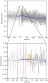Fig. 2. Timing residuals around the time of the glitch, as obtained in Palfreyman et al. (2018). Superimposed in blue, we plot our best fit for the residuals (Eq. (10) with the parameters of Table 1). In the zoomed-in part, we indicate the times t0, t1, t2 defined in Palfreyman et al. (2018) and our result for tmax (cf. Fig. 4). The glitch begins right after t1. Data points are connected by a line for clarity: in light grey those always omitted from the fit, in dark grey those always included, in orange the region corresponding to the interval of tcut over which we evaluate the parameters of the model, as explained in the text (cf. Fig. 3).

In order to decide how much data to neglect, we proceeded as follows: defining t_cut as the time before which the data are neglected, we performed the fit varying t_cut between t₂ − 1 s and t₂ + 4 s by steps of 0.1 s (the frequency of the Vela being about 11 Hz, this amounts to eliminating one data point at each successive fit). The fitted parameters can then be plotted as a function of t_cut: in Fig. 3, this is shown for $\mathrm{\Delta }{\mathrm{\Omega }}_p^{\infty }$ (the best determined parameter in our model, due to the extension of the data well after relaxation has completed). The fitted $\mathrm{\Delta }{\mathrm{\Omega }}_p^{\infty }$ first decreases until t_cut = t₂ + 0.5 s, then stabilises until t_cut = t₂ + 2 s, then decreases to stabilise at a slightly smaller value until t_cut = t₂ + 3 s. Short after that, the fitting of the data with expression (10), containing two exponentials, does not converge anymore, probably because too much data has been omitted to resolve the short time component and determine its parameters. The variations of $\mathrm{\Delta }{\mathrm{\Omega }}_p^{\infty }$ even during the stable phases shows the sensitivity of our fit to the choice of data range: even removal of one data point affects the result, which reflects the inherent noise in the timing residual data. We then decided to take, as final result for each parameter, the mean and standard deviations calculated from the values it assumes when t_cut varies in the interval [t₂ + 0.5 s, t₂ + 2 s]. We also checked that taking the mean and standard deviations in the longer interval [t₂ + 0.5 s, t₂ + 3 s] yields mean values within the previous errors and larger standard deviations (as obvious from the figure for $\mathrm{\Delta }{\mathrm{\Omega }}_p^{\infty }$). However, we prefer to adopt the smaller interval (for which the data points are marked in orange in Fig. 2), which eliminates less information about the short time component.

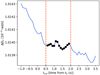Fig. 3. Results of the fit for the parameter $\mathrm{\Delta }{\mathrm{\Omega }}_p^{\infty }$ as a function of tcut, the time (measured with respect to t2) before which we neglect the data. We vary tcut by steps of 0.1 s, and connect the results by a line for clarity. Vertical lines define the region we chose to evaluate $\mathrm{\Delta }{\mathrm{\Omega }}_p^{\infty }$; the mean and standard deviations reported in Table 1 are taken for the values of $\mathrm{\Delta }{\mathrm{\Omega }}_p^{\infty }$ marked by black dots.

Although not compelling, the fact that $\mathrm{\Delta }{\mathrm{\Omega }}_p^{\infty }$ stabilises only five pulsar revolutions after t₂ seems to indicate that shortly after Δt_m, the magnetosphere recouples with the normal component. To our knowledge, no theoretical work on the decoupling and recoupling of the magnetosphere following a glitch has been performed, so that the timescale of order Δt_m = 2.6 s for the duration of this process remains, at present, only speculative. Incidentally, the recent work by Bransgrove et al. (2020) studies the response of the magnetosphere to a quake in the crust, arguing that this is the cause of the null pulse at t₀ and speculating that the quake may be the trigger of the glitch.

The data points were taken from Palfreyman et al. (2018) and they cover 72 min across the glitch: a part of them is shown in Fig. 2. The results for the seven independent parameters of Eq. (10) are reported in Table 1; in its lower part, we also show some dependent quantities, which can be derived from the equations in the previous section. The glitch, ΔΩ_p(t), and its (shifted) residuals, r(t) − r₀, corresponding to the parameters in the table are shown in Fig. 4, while the curve for the residuals r(t) is also superimposed to the data in Fig. 2.

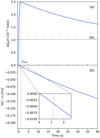Fig. 4. Upper panel: angular velocity with respect to the steady state, ΔΩp(t); lower panel: (shifted) residuals, r(t) − r0, corresponding to the values of the fitted parameters in Table 1. The flex in the residuals is marked by the intersection with the vertical line at tmax (see the zoom), and the time is measured from the beginning of the glitch.

The results of Table 1 yield some interesting considerations. First of all, the glitch size $\mathrm{\Delta }{\mathrm{\Omega }}_p^{\infty }$ is the same as what was obtained in Palfreyman et al. (2018) ($\mathrm{\Delta }{\mathrm{\Omega }}_p^{\infty }=1.006\cdot {10}^{-4}\text{rad}{\text{s}}^{-1}$) once their long-term (τ_d = 0.96 day) decay term ΔΩ_d = 0.008 × 10⁻⁴ rad s⁻¹ had been added (absent in our model, since the data we use extend to about 34 min after the glitch time).

Moreover, we find a decay timescale τ₊ = 43.3 ± 2.1 s, close to the shortest timescales measured in the 2000 and 2004 Vela glitches (Dodson et al. 2002, 2007) and within the errors of the value obtained in Ashton et al. (2019). The rise time τ₋ = 0.20 ± 0.14 s is over two orders of magnitude shorter than τ₊; it has quite large errors, reflecting the difficulty to resolve the short time behaviour, but it is well within the upper limit of 12.6 s determined by Ashton et al. (2019).

The mutual friction parameters B can be directly compared to the constraints given by Graber et al. (2018), namely 3 × 10⁻⁵ < ℬ_core < 10⁻⁴ for the drag between the core superfluid and the normal component, and ℬ_cr >  10⁻³ for that between the crustal superfluid and the normal component. These values possibly correspond to electron scattering off magnetised vortices in the core and kelvon scattering in the crust, the latter parameter being poorly predicted by theory, with differences of more than one order of magnitude at higher densities between different calculations (Graber et al. 2018).

If we interpret the two superfluid components of our model as the core (i = 1) and the crustal reservoir (i = 2), then the value ℬ₁ = (6.6 ± 0.6)×10⁻⁵ lies right in the constrained interval for ℬ_core; the parameter ℬ₂ is affected by a large error (reflecting the large uncertainty of all short time parameters, as seen in Table 1) but it also satisfies the lower limit on ℬ_cr. Since to date calculations of the drag coefficients ℛ_i have been uncertain, the present model provides a simple technique to extract average values of these parameters from glitch observations, which may help clarifying the theoretical issues concerning the microphysics involved in the dissipative channels at work during a glitch.

Regarding the time when the glitch begins, t_gl, our value is before what estimated in Palfreyman et al. (2018), but within their error bars. We find t_gl ≈ t₁, which supports the idea that the magnetosphere decoupling is associated to the onset of the glitch.

Finally, we discuss the fractional moments of inertia. In Fig. 5, we display the partial fraction of neutrons for shells starting from the surface and going deeper into the star, using a unified nucleonic equation of state (SLy4, Douchin & Haensel 2001) and for different values of the stellar mass. We see that the value x₂ ≈ 8% implies that the reservoir cannot be limited to the crust (which contains at most 4% of the neutron fraction for the lightest neutron star), but extends into the outer core to densities below nuclear saturation. For a standard 1.4 M_⊙ star, the intersection of the curve with the solid horizontal line representing x₂ in Fig. 5 shows that the reservoir extends to about 0.75n₀ (with n₀ = 0.168 fm⁻³ the nuclear saturation density); this is compatible with some calculations of S-wave pairing gaps (Ho et al. 2015; Montoli et al. 2020).

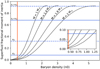Fig. 5. Moment of inertia fraction of neutrons enclosed in a spherical shell extending from the radius at which the neutron drip starts to the radius corresponding to a certain baryon number density. Baryon density corresponding to the internal boundary of the shell is given in units of n0 (nuclear saturation). Vertical line marks the core-crust transition at 0.45n0. Horizontal line represent x2 and x1 + x2 = 1 − xp without (solid lines: $m_1^{\ast }=m_2^{\ast }=1$) and with strong entrainment in the crust (dashed lines: $m_1^{\ast }=1,m_2^{\ast }=4$). We used the SLy4 equation of state and four reference masses: 1, 1.4, 1.8, and 2 M⊙. The inset is a zoomed-in image of the outermost regions of the core.

We also see that x₁ + x₂ ≈ 68%, implies that the moment of inertia fraction associated to normal matter is x_p ≈ 32%. This is much more than the value predicted by equations of state without an inner core (between 5% and 10%, as shown for SLy4 by the endpoints of the curves in Fig. 5, which give the total neutron fraction of the star, x_n, the remaining 1 − x_n then being the proton fraction). Therefore, our results suggest the presence of an inner core of matter strongly coupled to the charged component. For each mass in Fig. 5, the intersection of the curve with the solid horizontal line corresponding to x₁ + x₂ identifies the transition density to the innermost region that is rigidly coupled to the normal component. For a standard 1.4 M_⊙ star, such a core would start around 2n₀. This is compatible with microscopic calculations, which predict the appearance of an inner core of non-nucleonic matter (hyperons, meson condensates, quarks) at densities in the range 2n₀ − 3n₀. Other possibilities, however, can be proposed, such as strong coupling of the neutron superfluid to the proton superconductor in the inner core, due to the (still poorly known) vortex-fluxoid interaction.

4. Accounting for entrainment

In this section, we introduce entrainment, namely the non-dissipative coupling between the superfluid and the normal component (see e.g. Haskell & Sedrakian 2018; Chamel 2017). This can be represented by a dimensionless effective mass m^* of the free neutrons. The superfluid angular momentum for rigid rotation is given by a mixing between the superfluid and normal component J_n = I_n(m^*Ω_n + (1 − m^*)Ω_p), see for example, Andersson & Comer (2001) and Chamel & Carter (2006), and the dynamical Eqs. (1) become:

$$\begin{array}{c}\hfill \begin{array}{cc}& {\dot{\mathrm{\Omega }}}_p=-\frac{1}{x_p}(x_1{\dot{\mathrm{\Omega }}}_1+x_2{\dot{\mathrm{\Omega }}}_2+|{\dot{\mathrm{\Omega }}}_{\infty }|)\hfill \\ \hfill & m_1^{\ast }{\dot{\mathrm{\Omega }}}_1+(1-m_1^{\ast }){\dot{\mathrm{\Omega }}}_p=-x_p\frac{{\mathrm{\Omega }}_{1p}}{{\tau }_1}\hfill \\ \hfill & m_2^{\ast }{\dot{\mathrm{\Omega }}}_2+(1-m_2^{\ast }){\dot{\mathrm{\Omega }}}_p=-x_p\frac{{\mathrm{\Omega }}_{2p}}{{\tau }_2},\hfill \end{array}\end{array}$$(11)

where $m_{1,2}^{*}$ are the (averaged) effective masses for entrainment for the two superfluid components. The RHS of the equations for the superfluid in (11) are not effected by entrainment: this approximation holds under the same conditions valid for Eqs. (2) and (3), namely that the lags between the superfluids and the normal component are much smaller than the angular velocity of the normal component (cf. Eq. (52) for the vorticity density in Sidery et al. (2010), which reduces to 2Ω_i ≃ 2Ω_p(0) (i = 1, 2) when Ω_ip ≪ Ω_p(0)). Under such conditions, the (approximate) relation (3) still holds also in the presence of entrainment.

To solve the system (11), we introduced an auxiliary angular velocity, Ω_v, directly related to the vortex density by the Feynman-Onsager relation, and we properly rescaled the moments of inertia and the mutual friction coefficient with the effective mass. This way, the rescaled dynamical equations in the v-formalism are identical to those in the n-formalism without entrainment (Antonelli & Pizzochero 2017). In the case of our model with three rigid components, the Ω_vi are given by

$$\begin{array}{c}\hfill {\mathrm{\Omega }}_{\mathit{vi}}=m_i^{\ast }{\mathrm{\Omega }}_i+(1-m_i^{\ast }){\mathrm{\Omega }}_p(i=1,2),\end{array}$$(12)

which implies:

$$\begin{array}{c}\hfill {\stackrel{\sim }{\mathrm{\Omega }}}_{\mathit{ip}}={\mathrm{\Omega }}_{\mathit{vi}}-{\mathrm{\Omega }}_p=m_i^{\ast }{\mathrm{\Omega }}_{\mathit{ip}}(i=1,2).\end{array}$$(13)

The rescaled (tilded) variables are defined by:

$$\begin{array}{cc}& {\stackrel{\sim }{x}}_i=\frac{x_i}{m_i^{\ast }}(i=1,2)\hfill \end{array}$$(14)

$$\begin{array}{cc}& {\stackrel{\sim }{x}}_p=1-{\stackrel{\sim }{x}}_1-{\stackrel{\sim }{x}}_2=x_p-(1-m_1^{\ast }){\stackrel{\sim }{x}}_1-(1-m_2^{\ast }){\stackrel{\sim }{x}}_2\hfill \end{array}$$(15)

$$\begin{array}{cc}& {\stackrel{\sim }{\mathcal{B}}}_i=\frac{{\mathcal{B}}_i}{m_i^{\ast }}(i=1,2)\hfill \end{array}$$(16)

$$\begin{array}{cc}& {\stackrel{\sim }{\tau }}_i=\frac{{\tau }_i{m}_i^{\ast }{\stackrel{\sim }{x}}_p}{x_p}=\frac{{\stackrel{\sim }{x}}_p}{2{\mathrm{\Omega }}_p(0){\stackrel{\sim }{\mathcal{B}}}_i}(i=1,2),\hfill \end{array}$$(17)

where we used Eq. (3). By direct substitutions of Eqs. (12)–(17) in the system of Eqs. (11) and after some calculations, we finally obtain:

$$\begin{array}{c}\hfill \begin{array}{cc}& {\dot{\mathrm{\Omega }}}_p=-\frac{1}{{\stackrel{\sim }{x}}_p}({\stackrel{\sim }{x}}_1{\dot{\mathrm{\Omega }}}_{v1}+{\stackrel{\sim }{x}}_2{\dot{\mathrm{\Omega }}}_{v2}+|{\dot{\mathrm{\Omega }}}_{\infty }|)\hfill \\ \hfill & {\dot{\mathrm{\Omega }}}_{v1}=-{\stackrel{\sim }{x}}_p\frac{{\stackrel{\sim }{\mathrm{\Omega }}}_{1p}}{{\stackrel{\sim }{\tau }}_1}\hfill \\ \hfill & {\dot{\mathrm{\Omega }}}_{v2}=-{\stackrel{\sim }{x}}_p\frac{{\stackrel{\sim }{\mathrm{\Omega }}}_{2p}}{{\stackrel{\sim }{\tau }}_1},\hfill \end{array}\end{array}$$(18)

which is identical to the system of Eq. (1), but for the tilded variables.

It follows that, in the presence of entrainment, the timing solutions are still represented by Eqs. (4) and (10) for the glitch and its residuals, but with tilded parameters instead of untilded ones. Therefore, we do not need to repeat the fit: all the results reported in Table 1 are still valid, but they now represent the rescaled quantities. We can then go back to the physical variables using the previous relations: of course, the “observable” parameters (rise and decay timescale of the overshoot, amplitudes of the exponentials, $\mathrm{\Delta }{\mathrm{\Omega }}_p^{\infty }$, t_gl and r₀) remain the same, while only the “internal” parameters (fractional moment of inertia and mutual friction coefficients) must be rescaled. For example, we consider the case of no entrainment in the core component and strong entrainment in the reservoir; this is justified by some theoretical calculations, which suggest an effective mass slightly smaller than one in the core (Chamel & Haensel 2006), and quite large in the crust (Chamel 2012). In particular, we take $m_1^{*}=1$ and $m_2^{*}=4$, the latter being close to the average value of 4.3–4.3 (Andersson et al. 2012; Chamel 2013), but other values could be tested: to date, the issue of strong entrainment in the crust is still open to debate (Chamel 2012; Martin & Urban 2016; Watanabe & Pethick 2017; Sauls et al. 2020).

In Table 2, we report the physical quantities whose values are changed because of entrainment, namely the fractional moments of inertia and the mutual friction coefficients; with entrainment being confined to the crust (i = 2), only the values of the reservoir are affected, namely ${\mathcal{B}}_2=m_2^{\ast }{\stackrel{\sim }{\mathcal{B}}}_2$ and $x_2=m_2^{\ast }{\stackrel{\sim }{x}}_2$. In particular, the value of ℬ₂ = (1.1 ± 0.9)×10⁻¹ is four times larger than before and still satisfies the constraint of Graber et al. (2018); due to the mentioned uncertainty of theoretical calculations, no strong conclusion can be drawn at this stage. As for the fractional moments of inertia, the normal component now results x_p ≈ 8%, in agreement with standard neutron star models without an exotic inner core (indeed, in Fig. 5, the dashed horizontal line corresponding to x₁ + x₂ = 1 − x_p is very close to the endpoints of the curves for the neutron fraction). On the other hand, now the reservoir is x₂ ≈ 32%, a very large fraction extending into the outer core up to densities above nuclear saturation. For a standard 1.4 M_⊙ star, the intersection of the curve with the dashed horizontal line representing x₂ in Fig. 5 shows that the reservoir extends to about 1.25n₀. This suggests strong non-crustal pinning, possibly with the pasta phase and/or the magnetic fluxoids in the superconducting core, but other mechanisms could be envisaged.

5. Conclusions

We have presented the explicit, analytical timing solution for the minimal three-component model, which confirms the presence of an overshoot when the coupling timescales of the angular momentum reservoir are shorter than those of the superfluid core.

The fit of the 2016 Vela glitch with this model has provided several interesting physical quantities, like the rise and decay timescales of the overshoot, the time and amplitude of the glitch, and the fractional moments of inertia of the different components. We have compared our results with existing constraints derived from the 2016 Vela glitch, and found agreement with them.

We have studied the cases with and without strong entrainment in the crustal reservoir: in the former scenario, we find evidence of an inner core strongly coupled to the observable normal component and a reservoir extending beyond the crust up to densities below nuclear saturation; in the latter scenario, the normal component has standard values of fractional moment of inertia, but the reservoir extends deeper into the outer core, up to densities above nuclear saturation.

The explicit mathematical form of our model makes it possible to extract physical parameters of the neutron star directly from well-resolved (pulse to pulse) glitch observations in a reasonably simple way. This may help to clarify some presently open issues, like entrainment in the crust, mutual friction parameters, pinning in the pasta phase, and vortex-fluxoids interaction (Sourie & Chamel 2020).

It would also be interesting to study the possibility of both components being “active” (two distinct reservoirs of angular momentum), as well as to incorporate general relativistic corrections to the moments of inertia (Andersson & Comer 2001; Antonelli et al. 2018) and to the timescales (Sourie et al. 2017; Gavassino et al. 2020): we plan to address these issues in future work.

Acknowledgments

Partial support comes from PHAROS, COST Action CA16214 and INFN. Marco Antonelli acknowledges support from the Polish National Science Centre grant SONATA BIS 2015/18/E/ST9/00577 (PI: B. Haskell). We thank the anonymous referee and Brynmor Haskell for important suggestions which have improved our work.

References

All Tables

All Figures

	Fig. 1. Representation of a glitch with (β = 0.1) and without (β = 1.1) overshoot. The remaining parameters are taken from Table 1. Upper panel: angular velocity with respect to the steady state, ΔΩp(t), lower panel: (shifted) residuals, r(t) − r0. The flex in the residuals for the glitch with overshoot is marked by the intersection with the vertical line at t = tmax.
In the text

Fig. 2. Timing residuals around the time of the glitch, as obtained in Palfreyman et al. (2018). Superimposed in blue, we plot our best fit for the residuals (Eq. (10) with the parameters of Table 1). In the zoomed-in part, we indicate the times t0, t1, t2 defined in Palfreyman et al. (2018) and our result for tmax (cf. Fig. 4). The glitch begins right after t1. Data points are connected by a line for clarity: in light grey those always omitted from the fit, in dark grey those always included, in orange the region corresponding to the interval of tcut over which we evaluate the parameters of the model, as explained in the text (cf. Fig. 3).

In the text

Fig. 3. Results of the fit for the parameter $\mathrm{\Delta }{\mathrm{\Omega }}_p^{\infty }$ as a function of tcut, the time (measured with respect to t2) before which we neglect the data. We vary tcut by steps of 0.1 s, and connect the results by a line for clarity. Vertical lines define the region we chose to evaluate $\mathrm{\Delta }{\mathrm{\Omega }}_p^{\infty }$; the mean and standard deviations reported in Table 1 are taken for the values of $\mathrm{\Delta }{\mathrm{\Omega }}_p^{\infty }$ marked by black dots.

In the text

	Fig. 4. Upper panel: angular velocity with respect to the steady state, ΔΩp(t); lower panel: (shifted) residuals, r(t) − r0, corresponding to the values of the fitted parameters in Table 1. The flex in the residuals is marked by the intersection with the vertical line at tmax (see the zoom), and the time is measured from the beginning of the glitch.
In the text

Fig. 5. Moment of inertia fraction of neutrons enclosed in a spherical shell extending from the radius at which the neutron drip starts to the radius corresponding to a certain baryon number density. Baryon density corresponding to the internal boundary of the shell is given in units of n0 (nuclear saturation). Vertical line marks the core-crust transition at 0.45n0. Horizontal line represent x2 and x1 + x2 = 1 − xp without (solid lines: $m_1^{\ast }=m_2^{\ast }=1$) and with strong entrainment in the crust (dashed lines: $m_1^{\ast }=1,m_2^{\ast }=4$). We used the SLy4 equation of state and four reference masses: 1, 1.4, 1.8, and 2 M⊙. The inset is a zoomed-in image of the outermost regions of the core.

In the text

References

- Alpar, M. A., Pines, D., Anderson, P. W., & Shaham, J. 1984, ApJ, 276, 325 [NASA ADS] [CrossRef] [Google Scholar]
- Anderson, P. W., & Itoh, N. 1975, Nature, 256, 25 [NASA ADS] [CrossRef] [Google Scholar]
- Andersson, N., & Comer, G. L. 2001, CQG, 18, 969 [NASA ADS] [CrossRef] [Google Scholar]
- Andersson, N., Sidery, T., & Comer, G. L. 2006, MNRAS, 368, 162 [NASA ADS] [CrossRef] [Google Scholar]
- Andersson, N., Glampedakis, K., Ho, W. C. G., & Espinoza, C. M. 2012, Phys. Rev. Lett., 109, 241103 [NASA ADS] [CrossRef] [PubMed] [Google Scholar]
- Antonelli, M., & Pizzochero, P. M. 2017, MNRAS, 464, 721 [NASA ADS] [CrossRef] [Google Scholar]
- Antonelli, M., Montoli, A., & Pizzochero, P. M. 2018, MNRAS, 475, 5403 [NASA ADS] [CrossRef] [Google Scholar]
- Ashton, G., Lasky, P. D., Graber, V., & Palfreyman, J. 2019, Nat. Astron, 417 [Google Scholar]
- Baym, G., Pethick, C., Pines, D., & Ruderman, M. 1969, Nature, 224, 872 [NASA ADS] [CrossRef] [Google Scholar]
- Bransgrove, A., Beloborodov, A. M., & Levin, Y. 2020, ApJ, submitted [arXiv:2001.08658] [Google Scholar]
- Chamel, N. 2012, Phys. Rev. C, 85, 035801 [NASA ADS] [CrossRef] [Google Scholar]
- Chamel, N. 2013, Phys. Rev. Lett., 110, 011101 [NASA ADS] [CrossRef] [PubMed] [Google Scholar]
- Chamel, N. 2017, J. Low Temp. Phys., 189, 328 [NASA ADS] [CrossRef] [Google Scholar]
- Chamel, N., & Carter, B. 2006, MNRAS, 368, 796 [NASA ADS] [CrossRef] [Google Scholar]
- Chamel, N., & Haensel, P. 2006, Phys. Rev. C, 73, 045802 [NASA ADS] [CrossRef] [Google Scholar]
- Datta, B., & Alpar, M. A. 1993, A&A, 275, 210 [NASA ADS] [Google Scholar]
- Dodson, R., Lewis, D., & McCulloch, P. 2007, Ap&SS, 308, 585 [NASA ADS] [CrossRef] [Google Scholar]
- Dodson, R. G., McCulloch, P. M., & Lewis, D. R. 2002, ApJ, 564, L85 [NASA ADS] [CrossRef] [Google Scholar]
- Douchin, F., & Haensel, P. 2001, A&A, 380, 151 [NASA ADS] [CrossRef] [EDP Sciences] [Google Scholar]
- Espinoza, C. M., Lyne, A. G., Stappers, B. W., & Kramer, M. 2011, MNRAS, 414, 1679 [NASA ADS] [CrossRef] [Google Scholar]
- Gavassino, L., Antonelli, M., Pizzochero, P., & Haskell, B. 2020, MNRAS, in press, [arXiv:2001.08951] [Google Scholar]
- Graber, V., Cumming, A., & Andersson, N. 2018, ApJ, 865, 23 [NASA ADS] [CrossRef] [Google Scholar]
- Gügercinoğlu, E., & Alpar, M. A. 2014, ApJ, 788, L11 [NASA ADS] [CrossRef] [Google Scholar]
- Haskell, B., & Antonopoulou, D. 2014, MNRAS, 438, L16 [NASA ADS] [CrossRef] [Google Scholar]
- Haskell, B., & Melatos, A. 2015, Int. J. Mod. Phys. D, 24, 1530008 [NASA ADS] [CrossRef] [Google Scholar]
- Haskell, B., & Sedrakian, A. 2018, The Physics and Astrophysics of Neutron Stars (Switzerland AG: Springer Nature) Astrophys. Space Sci. Libr., 457, 401 [NASA ADS] [CrossRef] [Google Scholar]
- Haskell, B., Pizzochero, P. M., & Sidery, T. 2012, MNRAS, 420, 658 [NASA ADS] [CrossRef] [Google Scholar]
- Ho, W. C. G., Espinoza, C. M., Antonopoulou, D., & Andersson, N. 2015, Sci. Adv., 1, e1500578 [NASA ADS] [CrossRef] [Google Scholar]
- Link, B., Epstein, R. I., & Lattimer, J. M. 1999, Phys. Rev. Lett., 83, 3362 [NASA ADS] [CrossRef] [Google Scholar]
- Martin, N., & Urban, M. 2016, Phys. Rev. C, 94, 065801 [NASA ADS] [CrossRef] [Google Scholar]
- Montoli, A., Antonelli, M., & Pizzochero, P. M. 2020, MNRAS, 492, 4837 [NASA ADS] [CrossRef] [Google Scholar]
- Newton, W. G., Berger, S., & Haskell, B. 2015, MNRAS, 454, 4400 [NASA ADS] [CrossRef] [Google Scholar]
- Palfreyman, J., Dickey, J. M., Hotan, A., Ellingsen, S., & van Straten, W. 2018, Nature, 556, 219 [NASA ADS] [CrossRef] [Google Scholar]
- Pizzochero, P. M., Antonelli, M., Haskell, B., & Seveso, S. 2017, Nat. Astron., 1, 0134 [NASA ADS] [CrossRef] [Google Scholar]
- Sauls, J. A., Chamel, N., & Alpar, M. A. 2020, ArXiv e-prints [arXiv:2001.09959] [Google Scholar]
- Sidery, T., Passamonti, A., & Andersson, N. 2010, MNRAS, 405, 1061 [NASA ADS] [Google Scholar]
- Sourie, A., & Chamel, N. 2020, MNRAS, 493, L98 [NASA ADS] [CrossRef] [Google Scholar]
- Sourie, A., Chamel, N., Novak, J., & Oertel, M. 2017, MNRAS, 464, 4641 [NASA ADS] [CrossRef] [Google Scholar]
- Watanabe, G., & Pethick, C. J. 2017, Phys. Rev. Lett., 119, 062701 [NASA ADS] [CrossRef] [Google Scholar]
All Tables
Fractional moments of inertia and drag parameters obtained in the presence of strong entrainment in the reservoir ( and ).