| Issue |
A&A
Volume 636, April 2020
|
|
|---|---|---|
| Article Number | A45 | |
| Number of page(s) | 11 | |
| Section | Planets and planetary systems | |
| DOI | https://doi.org/10.1051/0004-6361/201936802 | |
| Published online | 15 April 2020 | |
A degree-100 lunar gravity model from the Chang’e 5T1 mission★
1
State Key Laboratory of Information Engineering in Surveying, Mapping and Remote Sensing, Wuhan University,
129 Luoyu Road,
430079 Wuhan, PR China
e-mail: This email address is being protected from spambots. You need JavaScript enabled to view it.
2
Observatoire de la Côte d’Azur, Geoazur, CNRS UMR7329,
Valbonne, France
e-mail: This email address is being protected from spambots. You need JavaScript enabled to view it.
3
Chinese Antarctic Center of Surveying and Mapping, Wuhan University,
129 Luoyu Road,
430079
Wuhan,
PR China
4
National Key Laboratory of Science and Technology on Aerospace Flight Dynamics, Beijing Aerospace Flight and Control Center,
100094 Beijing, PR China
5
Space Science Institute, Macau University of Science and Technology,
Avenida Wailong Taipa,
999078
Macau, PR China
6
Observatoire géodésique de Tahiti, University of French Polynesia,
98702 Faa’a,
BP 6570 Tahiti,
French Polynesia, France
Received:
28
September
2019
Accepted:
4
March
2020
Abstract
Context. Chinese lunar missions have grown in number over the last ten years, with an increasing focus on radio science investigations. In previous work, we estimated two lunar gravity field models, CEGM01 and CEGM02. The recently lunar mission, Chang’e 5T1, which had an orbital inclination between 18 and 68 degrees, and collected orbital tracking data continually for two years, made an improved gravity field model possible.
Aims. Our aim was to estimate a new lunar gravity field model up to degree and order 100, CEGM03, and a new tidal Love number based on the Chang’e 5T1 tracking data combined with the historical tracking data used in the solution of CEGM02. The new model makes use of tracking data with this particular inclination, which has not been used in previous gravity field modeling.
Methods. The solution for this new model was based on our in-house software, LUGREAS. The gravity spectrum power, post-fit residuals after precision orbit determination (POD), lunar surface gravity anomalies, correlations between parameters, admittance and coherence with topography model, and accuracy of POD were analyzed to validate the new CEGM03 model.
Results. We analyzed the tracking data of the Chang’e 5T1 mission and estimated the CEGM03 lunar gravity field model. We found that the two-way Doppler measurement accuracy reached 0.2 mm s−1 with 10 s integration time. The error spectrum shows that the formal error for CEGM03 was at least reduced by about 2 times below the harmonic degree of 20, when compared to the CEGM02 model. The admittance and correlation of gravity and topography was also improved when compared to the correlations for the CEGM02 model. The lunar potential Love number k2 was estimated to be 0.02430±0.0001 (ten times the formal error).
Conclusions. From the model analysis and comparison of the various models, we identified improvements in the CEGM03 model after introducing Chang’e 5T1 tracking data. Moreover, this study illustrates how the low and middle inclination orbits could contribute better accuracy for a low degree of lunar gravity field.
Key words: Moon / gravitation / planets and satellites: detection / methods: data analysis
Data and models are only available at the CDS via anonymous ftp to cdsarc.u-strasbg.fr (130.79.128.5) or via http://cdsarc.u-strasbg.fr/viz-bin/cat/J/A+A/636/A45
© ESO 2020
1 Introduction
The study of the lunar gravity field has developed rapidly over the last half century. The Luna 10 mission from the Soviet Union and Lunar Orbiter 1 mission from the United States launched in 1966 heralded the beginning of lunar gravimetric research (Akim 1967). Using the tracking data from Lunar Orbiter 2 in 5 missions in 1967, Lorell & Sjogren (1968) presented a preliminary gravity model that included a set of harmonic coefficients through degree 8 in the zonal and degree 4 in the tesserals. Combining these data with those from the Apollo 15 and 16 missions, Bills & Ferrari (1980) presented a lunar gravity field model with degree and order of 16. In the 1990s the Clementine and Lunar Prospector (LP) missions enhanced lunar gravity field recovery at a high-resolution degree and order. Based on the LP100J lunar gravity field model, Konopliv et al. (2001) calculated the LP165P lunar gravity field model with a degree and order of 165 by exploiting LP tracking data collected during the LP extended mission phase. Going into the 21st century, the Japanese SELenological and Engineering Explorer (SELENE) mission raised the study of the lunar gravity field and interior structure to a new level.
In the SELENE mission, the Rstar relay satellite provided direct Doppler shift measurements from the farside gravity field for the first time. Namiki et al. (2009) derived the SGM90d using the first three months of SELENE tracking data. By integrating the four-way Doppler measurement data from the SELENE mission collected over one year, Matsumoto et al. (2010) estimated a gravity field model with a degree and order of 100, SGM100h. Following the SELENE mission, NASA’s Gravity Recovery and Interior Laboratory (GRAIL) mission was launched in 2011. It was designed to accurately map the lunar gravity from low to very high wavelengths from a polar orbit (Zuber et al. 2012). Only using three months of primary mission phase data from GRAIL, Zuber et al. (2013) published a gravity field model, GL0420A, up to a degree and order of 420. Meanwhile, the Jet Propulsion Laboratory (JPL) and Goddard Space Flight Center (GSFC) developed the GL0660B model (Konopliv et al. 2013) and the GRGM660PRIM model (Lemoine et al. 2013) each with degree and order of 660. After adding the tracking data from GRAIL’s extended phase mission, JPL and GSFC published two additional gravity field models, GL0900D (Konopliv et al. 2014) and GRGM900C (Lemoine et al. 2014), up to a degree and order of 900. After that, two gravity field models with a degree and order of 1500 (Park et al. 2015) and 1200 (Goossens et al. 2016) were separately calculated by JPL and GSFC. Although the study of lunar gravity fields has risen to unprecedented heights, other research groups are still working on gravity field recovery from different views.
With the help of the orbit products (GNI1B) provided by the GRAIL Science Team, Arnold et al. (2015) released two lunar gravity field models up to degree 200, AIUB-GRL200A/B. Klinger et al. (2014) provided the Graz lunar gravity fieldmodels, GrazLGM200a, which relies on the official orbit data retrieved from GNI1B. Wirnsberger et al. (2019) presented the first completely independent Graz lunar gravity model compiled with no involvement of the GRAIL Science Team, denoted GrazLGM420b. They estimated this gravity field model based on an in-house software package, the Orbit Re-Construction Application. The Chinese lunar exploration program has been going for over 10 yr, beginning with the Chang’e 1 mission launched in 2007 (Wei et al. 2018). Regardless of the limited accuracy and coverage of tracking data from the Chang’e 1 mission, a lunar gravity field model, CEGM01, up to degree and order 50 was estimated using one year of tracking data (Yan et al. 2010). A new gravity field model CEGM02 with degree and order of 100 was developed (Yan et al. 2012) using the Chang’e 1 orbital tracking data in combinationwith orbital tracking data from SELENE, LO-I to LO-V, Apollo 15 and 16, Clementine, LP, and SMART-1 (hereafter historical spacecraft). These two solutions for the gravity field model were estimated using the GSFC GEODYN-II package (Pavlis et al. 2006). The details of their derivation are given in Table 1. Moreover, based on the GRAIL mission, many local solutions for lunar gravity fields have also been derived (Goossens et al. 2020, 2018, 2014).
As shown in Table 1, the GRGM series models have already reached an unprecedented level of accuracy and resolution with the inclusion of the GRAIL data set. Although the GRGM series models have very high resolution, there are still discrepancies in the low degree coefficients and long-wavelength components of the solutions developed by two space research centers (JPL and GSFC) (Yan et al. 2018). The fourth Chinese lunar probe, Chang’e 5T1, was launched on October 23, 2014, with the goal of testing the Earth atmosphere reentry technology. It is still orbiting the Moon at the time of writing. In this study, we present a new lunar long-wavelength gravity model, CEGM03, including tracking data from the Chang’e 5T1 mission and the historical tracking data used in the solution of CEGM02.
This Chang’e 5T1 mission collects long-period radio tracking data, unlike previous Chinese missions. During tracking by Chang’e 5T1, there were fewer maneuvers than during the Chang’e 1 mission. In addition, the inclination of Chang’e 5T1 is about 18–68°, which is very different from the polar orbits employed in previous lunar gravity field solutions. Another highlight of this work is that our new gravity field model was solved based on our in-house software, LUGREAS (Ye et al. 2016), which we thoroughly validated via the GEODYN-II software as a reference on precision orbit determination (POD). With the help of the Chang’e 5T1 tracking data, we also derived a solution for the k2 value.
A brief summary of this paper is as follows. In Sect. 2 we describe the Chang’e 5T1 mission, focusing on technical details and orbits. In Sect. 3 we present the methods and procedures used for the gravity modeling from the Chang’e 5T1 Doppler data. In Sect. 4 we assess the accuracy of CEGM03 in multiple ways. We summarize and make some concluding remarks in Sect. 5.
Classical gravity field models and their data sources.
2 Chang’e 5 tracking data
2.1 Description of orbits
The Chang’e 5 T1 spacecraft was launched at 18:00 UTC on October 23, 2014, from the Xichang Satellite Launch Center. The separation between the service module and the Earth return vehicle was executed on October 31, 2014. The service module carried out the Moon mission, as well as a series of extended experiments (see Fig. 1).
As illustrated in Fig. 1, the service module started its extended mission after separation, which included three orbital phases: high eccentric parking orbit, trans-lunar orbit, and a Lissajous trajectory in the vicinity of the Earth-Moon Lagrange point L2. The probe continued to orbit the Moon after concluding the extension mission. Figure 2 shows the state of the Chang’e 5T1 spacecraft in terms of mass (a), orbit inclination (b), and eccentricity (c), from October 2014 to December 2016; the tracking data were used to estimate a new lunar gravity field model after the extended mission. During the extension mission, the orbit of Chang’e 5T1 at middle inclination was a relatively stable orbit with an eccentricity of approximately 0.02, and it was close to circular like the orbit of the Chang’e 1 spacecraft. A combination of orbit inclinations and eccentricities like this has never been tried for a lunar gravity field modeling mission. In the next chapter, we present the radio tracking data set used to estimate our lunar gravity field model.
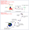 |
Fig. 1 Experimental mission orbits of the Chang’e 5 T1 spacecraft. |
2.2 Observation strategies and data set
To support the Chang’e 5T1 mission, the Chinese Deep Space Network (CDSN) and Chinese Very long baseline interferometry Network (CVN) have upgraded in performance and provided continuous tracking for the spacecraft, as shown in Fig. 3. We should mention that there are two antennas at the Kashi station (KS), named KS1 and KS2, for Chang’e 5T1. There is a small difference in coordinates between these two antennas.
During whole mission, S-band radio links were used to obtain tracking data. The closed-loop S-band round-trip signal was received and coherently transponded by phase-lock-loop. The tracking data used to estimate a new lunar gravity field period are plotted in Fig. 4.
During the tracking period shown in Fig. 4, when the Chang’e 5T1 spacecraft was in a routine orbit of the Moon, the Argentina station was not used for tracking. In 2015, four tracking stations, KS1, KS2, JMS, and QD, worked together. After May 2016, only the JMS and KS1 antennas were used to track the spacecraft. The effects of ionospheric and tropospheric corrections in the observation data were removed using co-located GPS observations and meteorological data. The sampling rate of two-way Doppler was one second, while filtered Doppler data at intervals of 10 s were used in the research discussed in this paper.
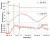 |
Fig. 2 Time evolution of the Chang’e 5 T1 spacecraft’s mass (a), orbit inclination (b), and eccentricity (c). The green shaded areas in this graph indicate the trajectory-correction maneuvers. At the beginning the maneuvers are frequentwith abrupt mass losses, after which the mass change slowly. The inclination oscillates between 18 and 68 degrees, which is different from the Chang’e 1 probe (from 87 to 91 degrees). The eccentricity evolution is small (below 0.05) in the orbiting period, and a stable orbit is maintained. |
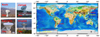 |
Fig. 3 Chinese stations: geographical distribution of CDSN and CVN sites. Red spots indicate Chinese radio tracking stations and yellow spots VLBI stations. In China the CDSN includes two stations at Qingdao (QD) with 18 m antennas, one at Kashi(KS) with a 35 m antenna, and one at Jiamusi (JMS) with a 66 m antenna; in Argentina there is one station with an antenna diameter of 35 m. Each site is indicated by a red point on the map. The CVN includes four stations, one each at Urumqi (25 m antenna), Kunming (40 m antenna), Beijing (50 m antenna), and Shanghai (65 m antenna). Background: https://ngdc.noaa.gov/mgg/image/color_etopo1_ice_low.jpg |
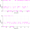 |
Fig. 4 Tracking time span from CDSN. Purple points indicate effective tracking time, and the blank spaces indicate no observations. |
3 Gravity field recovery
3.1 Dynamic modeling in POD
Dynamic orbit determination and gravity field recovery relies on the integration of the equation of motion in inertial space, and the equation for the motion dynamics of the Chang’e 5T1 spacecraft. We refer to Moyer (1971).
The lunar gravity potential V is given in a body fixed reference frame in terms of spherical harmonics expansion (Heiskanen & Moritz 1967; Hobson 1931), as
![Mathematical equation: \begin{equation*} \begin{split} V(r, \psi,\lambda)=&\frac{GM}{R}\sum_{n=0}^{N_{\textrm{max}}}\left(\frac{R}{r}\right)^{n+1} \sum_{m=0}^{N_{\textrm{max}}} \overline{P}_{nm} ({\textrm{sin}}\psi)\\[3pt] & (\overline{C}_{nm}{\textrm{cos}}(m\lambda)+\overline{S}_{nm}\textrm{sin}m\lambda)) \end{split},\end{equation*}](/articles/aa/full_html/2020/04/aa36802-19/aa36802-19-eq1.png) (1)
(1)
where r, ψ, and λ are the height, latitude, and longitude of the spacecraft; GM is the gravitational parameter of the Moon with the reference radius R of 1738 km;  is a latitude dependent function and indicates the normalized associated Legendre functions of degree n and order m; and
  and
and  are the corresponding spherical harmonics coefficients. In this study Nmax is the maximum spherical harmonic degree, which is 100.
The spacecraft is subject to acceleration induced by direct solar radiation pressure as well as small perturbative acceleration due to sunlight reflected from the lunar surface. In addition to the indirect radiation pressure, thermal infrared emission from the lunar surface should also be considered. In computing the albedo and emissivity, LUGREAS uses the Knocke second-degree zonal spherical harmonic representation of the lunar albedo and emissivity. Detailed information can be found in the GEODYN Systems Description (Pavlis et al. 2006). We introduced empirical parameters with a priori assigned stochastic properties to account for mismodeled or unmodeled non-gravitational accelerations. The empirical accelerations are estimated per arc with a priori amplitudes of 10−9 m s−2.
3.2 Computing environment
A flowchart with details for all LUGREAS modules is shown in Fig. 5. The prediction and batch modules are the core processing parts of this software. The prediction part focuses on force model building, an integrator configuration, and related parameter initializations, while the batch part carries out matrix allocation, storage, calculation of observation residuals, and inversion of normal equations.
The numeric integrator combines dynamic and variational equations, as illustrated in the flowchart shown in Fig. 5. The solution parameters can be divided into global and arc-related parameters. The global parameters include lunar gravity field model coefficients and k2 values. The arc parameters include empirical accelerations, S-band measurement bias, and initial orbital elements. These parameters are estimated using weighted least-squares batch processing. During the derivation of arc parameters, the LUGREAS generates a normal matrix of global parameters. Each normal matrix for every arc is stacked to estimate the global parameters (Kaula 1966). The whole process is iterated to obtain a converged solution. In the next section, we present the detailed LUGREAS configurations used for the Chang’e 5T1 data processing.
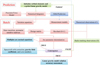 |
Fig. 5 Computation chain for lunar gravity field in LUGREAS software. A 12-order Adams-Cowell prediction-correction integrator (Thornton & Border 2003) is used to obtain the spacecraft ephemeris, the state transition matrix and the parameter sensitivity matrix. The C means theoretical values. Observations provided by Earth tracking stations are labeled O. |
Configurations for POD and gravity field recovery in LUGREAS.
3.3 Configurations
We determined a lunar gravity field model based on Chang’e 5T1 spacecraft from 2015 to 2016. The arc length was set to one day depending on the unrecorded time of the momentum wheel during spacecraft tracking. Table 2 summarizes all the dynamic models, correction models, and estimated parameters.
In Table 2, the dynamic models include a priori lunar gravity field (SGM100g), N-body perturbations, perturbations stemming from Earth-Moon oblateness, relativity perturbations, solid tidal perturbations, and solar radiation. The DE421 ephemerides was used to obtain the positions of all planets, and to define the lunar reference system in which we estimate the gravity field (Williams et al. 2008). The correction model incorporates relativistic acceleration correction, Earth tropospheric correction, TDB-TT translation model in light time calculation, and tracking station coordinate correction.
The parameters we estimated can be conveniently divided into arc and global parameters. The arc parameters are those that influence only the data in an arc, and global parameters are those that influence all data. The arc parameters include the initial orbital elements of the Chang’e 5T1 spacecraft, three-axis empirical accelerations, and S-band two-way Doppler measurement biases. The pass-dependent biases of the two-way Doppler were estimated to account for measurement modeling errors. The global parameters include lunar gravity field coefficients up to degree and order 100, and the degree 2 tidal Love number k2. Of note, we used the CEGM02 covariance matrix in the solution, which means we adopted the Kaula constraint indirectly. The initial orbital elements were retrieved from a reconstructed initial ephemeris of the Chang’e 5T1 provided by Beijing Aerospace Control Center.
In our combined solution, the weight of the Chang’e 5T1 two-way Doppler was set to 1 cm s−1 for a Doppler window of 10 s. In addition to the two-way Doppler tracking data from the Chang’e 5T1 orbiting mission, we also combined the orbital tracking data of Chang’e 1 and other historical spacecraft that were used in estimating SGM100h. The weights of the data used in solving the CEGM03 model are provided in Table 3. The details of the data and processing for Chang’e 1 and other historical spacecraft can be found in Yan et al. (2012) and Matsumoto et al. (2010), respectively. The estimated solution is discussed in Sect. 4.
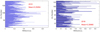 |
Fig. 6 DSN S-band Doppler post-fit residuals per arc in terms of root mean square (RMS). |
4 Results and discussion
4.1 Residuals analysis
For our gravity model, 308 arcs were collected altogether. In 2015, the CDSN tracked Chang’e 5T1 for 246 days and we obtained 182 arcs, which can be used in the solution of gravity field model. In 2016, Chang’e 5 T1 was tracked for about 202 days and we achieved 126 arcs. There are two factors leading to rejected arcs. The first is a large orbital maneuver or too few observationsin the arc. The second is loss of information on spacecraft outgassing or possible propulsion leaks in original data records. Figure 6 shows the post-fit residuals of the 308 arcs used in our CEGM03 solution.
In Fig. 6, we can see that the mean values of the Doppler residual RMS were about 0.29 mm s−1 for 2015 and 2016, compared to 4 mm s−1 of the Chang’e 1 Doppler tracking data (Yan et al. 2010). Actually, for most of the arcs, the RMS of post-fit residuals was about 0.2 mm s−1. The Chang’e 5T1 Doppler residual results show improved performance in tracking accuracy and CDSN stability.
Summary of tracking data used in the CEGM03 model.
4.2 Power spectrum of lunar gravity field model coefficients
We used a power spectrum to represent the accuracy of the CEGM03 model. The RMS coefficient sigma degree variance σn is labeled “σ” and RMS coefficient error degree variance δn is labeled “δ”. The formulas used for computing these values are as follows (Kaula 2013):
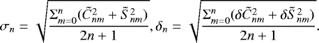 (2)
(2)
Here  and
and  are error variances of the normalized Stokes coefficients
  and
and  , respectively. The RMS coefficient sigma degrees variances show the frequency intensity of the gravity field model. The RMS coefficient error degree variances are formal errors retrieved from the posteriori covariance matrix of the model. Figure 7 shows the power spectrum curves of the SGM100h, CEGM02, and CEGM03.
The variance curve of the RMS coefficient error degree in Fig. 7 shows that the Chang’e 5 T1 orbit tracking data mostly contribute to lower degree and order coefficients. The orbital height of Chang’e 5 T1 ranged from about 195 to 200 km, which was similar to the Chang’e 1 orbital height of about 200 km, so they were not as sensitive to short-wavelength gravity information as the GRAIL mission. Thus, CEGM03 coefficients with a degree and order higher than 25 were calculated mainly fromLP data and SELENE data. The contributions from Chang’e 5 T1 were concentrated in the lower degrees and orders, in contrast to the CEGM02 and SGM100h gravity field models. Below degree 5, the formal error in the CEGM02 model was reduced by a factor of about two relative to the SGM100h model, while below degree 20 the formal error for the CEGM03 model was reduced by a factor of about 2 compared to the CEGM02 model.
Together with the gravity coefficients, we also estimated the k2 value, which was found to be 0.02430 ± 0.0001 (ten times the formal error). This value agrees with the averaged k2 solutions from previous missions (0.02416 ± 0.00022; see Williams et al. 2014; Williams & Boggs 2015; 0.02427±0.0004 (ten times the formal error), see Yan et al. 2012). The GM value is 4902.801743 ± 0.637 × 10⁻³ km3 s−2.
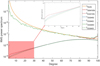 |
Fig. 7 Power spectra of gravity field solutions. Solid lines: signal degree-RMS (labeled “σ”) and dashed lines: formal error degree-RMS (labeled “δ”); the orange solid line corresponds to Kaula’s rule, 3.6 × 10⁻⁴∕l2. |
4.3 Gravity anomalies
Gravity anomalies are a major source of data in studying the lunar internal structure. The Free-Air gravity Anomalies (FAA) is defined as
![Mathematical equation: \begin{eqnarray*} \textrm{FAA}(r,\phi,\lambda)&=&\frac{\partial{V}}{\partial{r}}-\frac{2V}{r}\nonumber\\[3pt] &=&\frac{GM}{r^2}\sum_{n=0}^{N_{\textrm{max}}}(n-1)\left(\frac{R}{r}\right)^n \sum_{m=0}^{n}\overline{P}_{nm}({\textrm{sin}}\psi)(\overline{C}_{nm}{\textrm{cos}}(m\lambda)\nonumber\\[3pt] &&+\,\overline{S}_{nm}\textrm{sin}m\lambda)). \end{eqnarray*}](/articles/aa/full_html/2020/04/aa36802-19/aa36802-19-eq10.png) (3)
(3)
The FAA values are computed with respect to a reference sphere with radius of 1738.0 km (R), and with full expansion degree and order up to 100. V represents the lunar gravity potential. For explanation of the other parameters see Eq. (1). Figure 8 shows the FAA for the CEGM03 and CEGM02 models.
There are slight differences in gravity anomalies between the CEGM02 and CEGM03 gravity field models, which reflect lateral variations in lunar internal mass and density distributions. The color scale is truncated at about ±400 mGal, while the maximum and minimum anomalies in the CEGM03 model were 646 and −776 mGal located at (32.079° E, 85.545° S) and (273.564° E, 80.198° S), respectively. On the far side, however, the resolution of gravity anomalies remains low, since the amount of the farside tracking data employed in the CEGM03 and CEGM02 solution is still limited. The SELENE farside tracking data were used, and no new farside tracking data were added to solve the CEGM03 model.
The respective quality of the CEGM02 and CEGM03 gravity models can be partially assessed using the formal standard deviation maps of the gravity anomaly error and selenoid error maps (Fig. 9), computed from the posterior covariance matrix of each model, up to degree and order 30. The RMS value is 0.256 and 0.221 mGal respectively for CEGM02 and CEGM03, and 0.121 and 0.103 m for the selenoid undulations. We also calculated the global RMS of anomaly error and selenoid error up to degree n, with n = 2, …, 30. Figure 10 shows the evolution of the error spectrum of CEGM02 and CEGM03 with the harmonic degree (solid lines). We can see that the CEGM03 model performs better than the CEGM02 model. It should be noted that we cut off the degree and order 30, since this new lunar gravity model improvement on the low degree is more significant than the high degree.
To further study the influence of the orbit inclination on the new gravity model1, the correlations between the zonal coefficients and the other coefficients are shown in Fig. 11. The correlation values for the CEGM03 model (Chang’e 5T1 orbit inclinations from 18 to 68 degrees) are a little smaller than the CEGM02 model overall (the Chang’e 1 orbit was nearly polar).
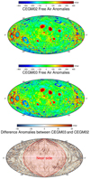 |
Fig. 8 From top to bottom: maps of the free-air gravity anomalies of CEGM02 and CEGM03, and the differences between CEGM03 and CEGM02. The maps are centered on 0°E longitude (Hammer projection). |
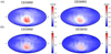 |
Fig. 9 Gravity anomaly error distribution (a) and selenoid error distribution (b) at degree n = 30. The maps are centered at 180° E and with the Hammer projection. |
4.4 Correlation with topography
For the Moon, the high degree of gravity anomalies stem predominantly from uncompensated topography. In this section, our CEGM03 model is evaluated using admittance and correlations with respect to the Lunar Reconnaissance Orbiter (LRO) topography model LRO_LTM05_2050_SHA.TAB (Smith et al. 2010). The admittance and correlations are computed according to Wieczorek (2007), which can indicate lunar isostatic compensation. If we define Sff (l) and Sgg (l) as the power of topography f and gravity g, respectively, and Sfg (l), as their total cross-power spectrum, the gravity/topography admittance Z(l) and correlation spectrum γ(l) at degree l are computed as
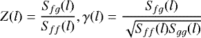 (4)
(4)
Gravity and topography are independent when the correlation has the relationship γ(l) = 0. In general, a higher correlation between topography and gravity point to better models (Lemoine et al. 2001; Han et al. 2009). Four gravity field models are presented in Fig. 12: GRGM660, SGM100h, CEGM02, and CEGM03.
The CEGM03 model yields higher admittances and correlations with topography in the degree and order 80–100 range with respect to the CEGM02 and SGM100h models (Fig. 12a). The GRGM660 GRAIL model performs better, due to the gradiometer nature of the gravity measurement for this model. A negative correlation arises at degree 10, and is certainly related to the presence of the nearside mascons (Fig. 12b).
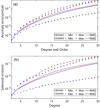 |
Fig. 10 Gravity anomaly error (a) and selenoid error (b) from 2 to 30 degree and orders. Solid lines: the RMS of global anomaly error or selenoid error; plus signs: minimum value of global anomaly error or selenoid error; stars: maximum value of global anomaly error or selenoid error. |
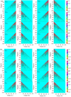 |
Fig. 11 Correlation between the zonal coefficients and other harmonic coefficients of the gravity models, CEGM02 (a) and CEGM03 (b). For each plot the left part is the correlation between the zonal coefficients and Cnm coefficients, and the right part is the correlation between the zonal coefficients and Snm coefficients. |
4.5 Orbital performance
In this section, we compare the performance of the CEGM03 model with other gravity field models, GRGM660, SGM100h, and CEGM02, in terms of orbit determination for Chang’e 5T1. The maximum degree and order expansion for each gravity field model is limited to degree and order 100. It should be noted that the GRAIL model is tailored to the modeling of high degree and order coefficient. The selected arcs span the period from 25 May to 25 July 2015. Figure 13 summarizes the per-arc post-fit residual RMS values, and the orbit determination software used was LUGREAS.
From Fig. 13 we can see the mean RMS of post-fit residuals is about 0.37 mm s−1 for the GRGM660 gravity field model. The corresponding post-fit residuals are about 0.43 mm s−1 for the CEGM03 model, 0.66 mm s−1 for SGM150, and 0.72 mm s−1 for CEGM02. Figure 14 shows the orbit overlaps of the Chang’e 5T1. Overlaps mean that we extended one-day arcs constrained by observations by 12 h (unconstrained) to compare them with the one-day (constrained) neighboring arcs.
We can see in Fig. 14 that there are significant improvements in the CEGM03 model in the along-track component direction when compared with the CEGM02 and SGM100h models. There are no improvements when comparing CEGM03 overlaps with GRGM660 overlaps. It should be noted that the SGM100h and CEGM02 models for the orbit determination have strong similar points because of the similar data used. With the Chang’e 5T1 data combining, it contributes to improving the accuracy of orbit determination for low and middle orbital spacecraft. The average values of the overlaps are listed in Table 4.
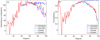 |
Fig. 12 Admittance (a) and correlation (b) between several lunar gravity field solutions and gravity induced from topography. |
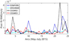 |
Fig. 13 Post-fit residual RMS for the Chang’e 5 T1 based on different gravity field models, considering that some unrecorded maneuvers occurring when tracking data for 25 arcs were selected. |
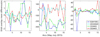 |
Fig. 14 Average differences of orbit overlaps in R (radial), N (normal), and T (tangential) directions. |
Average differences in R (radial), N (normal), and T (tangential) directions for the selected 16 overlaps.
5 Conclusion
The present study introduces a new solution, CEGM03, for the lunar gravity field model using the Chang’e 5T1 mission data. During the POD, we found that the two-way Doppler measurements post-fit residuals could reach the 0.2 mm s−1 level for a Doppler window of 10 s for most of the arcs, while the noise level of the Chang’e 1 mission was about 4 mm s−1 for the sameDoppler window. The CEGM03 model outperforms the SGM100h and CEGM02 models for Chang’e 5T1 orbit determination, but is outperformed by the GRGM660 model for this task. Nevertheless, our CEGM03 model is built from a wide range of orbit inclinations (18 and 68 degrees) of the Chang’e 5T1 spacecraft, while the GRGM660 model uses only polar orbits.This work demonstrates that our CEGM03 model is state-of-the-art in its ability to extract gravity information from two-way Doppler tracking. The next step is, without doubt, to combine Chang’e 5 Doppler tracking data with its unique range of orbital inclination with the Doppler and gradiometric tracking from GRAIL or GRAIL-like polar-orbit future missions, to obtain a highly precise lunar gravity field at all wavelengths and a better k2 estimate.
In the near future, China will continue to launch lunar missions, including Chang’e 5/6/7/8. The CDSN plans to use X or Ka band measurement, and employ highly precise ground atomic clocks. These missions will provide more accurate and stable orbital tracking data, making it possible for us to make further improvements to the long wavelengths of the lunar gravity field and k2 solutions.
Acknowledgements
We are grateful to the Chinese deep space network for providing models and data to make this research possible. We appreciated the discussion with Prof. Jinsong Ping from the National Astronomical Observatory of China, and we thank Mr. Stephen C. McClure, a native English speaker and researcher, from Wuhan University for helping polish this paper. The work is supported by the National Natural Science Foundation of China (U1831132, 41874010, 41804025), the Innovation Group of Natural Fund of Hubei Province (2018CFA087), and the Science and Technology Development Fund of the Macau Special Administrative Region (007/2016/A1, 119/2017/A3, 187/2017/A3). This work is also supported by the Open Funding of Macau University of Science and Technology (FDCT 119/2017/A3). J.-P.B. was funded by a DAR grant in planetology from the France Space Agency (CNES). The numerical calculations in this paper were done at the Supercomputing Center of Wuhan University. We are grateful to the anonymous referee for helpful comments that improved the manuscript.
References
- Akim, E. L. 1967, Sov. Phys. Dokl., 11, 855 [NASA ADS] [Google Scholar]
- Arnold, D., Bertone, S., Jäggi, A., Beutler, G., & Mervart, L. 2015, Icarus, 261, 182 [NASA ADS] [CrossRef] [Google Scholar]
- Bills, B. G., & Ferrari, A. J. 1980, J. Geophys. Res. Solid Earth, 85, 1013 [CrossRef] [Google Scholar]
- Davis, J., Herring, T., Shapiro, I., Rogers, A., & Elgered, G. 1985, Radio Sci., 20, 1593 [NASA ADS] [CrossRef] [Google Scholar]
- Goossens, S., Matsumoto, K., Kikuchi, F., et al. 2011, Improved High-Resolution Lunar Gravity Field Model From SELENE and Historical Tracking Data, AGU Fall Meeting, P44B-05 [Google Scholar]
- Goossens, S., Sabaka, T. J., Nicholas, J. B., et al. 2014, Geophys. Res. Lett., 41, 3367 [NASA ADS] [CrossRef] [Google Scholar]
- Goossens, S., Lemoine, F., Sabaka, T., et al. 2016, Lunar Planet. Sci. Conf., 47, 1484 [NASA ADS] [Google Scholar]
- Goossens, S., Sabaka, T., Fernández Mora, A., & Heijkoop, E. 2018, Lunar Planet. Sci. Conf., 49, 2477 [NASA ADS] [Google Scholar]
- Goossens, S., Sabaka, T., Wieczorek, M., et al. 2020, J. Geophys. Res. Planets, 125, e2019JE006086 [NASA ADS] [CrossRef] [Google Scholar]
- Han, S.-C., Mazarico, E., & Lemoine, F. G. 2009, Geophys. Res. Lett., 36, L11203 [NASA ADS] [CrossRef] [Google Scholar]
- Heiskanen, W., & Moritz, H. 1967, Physical Geodesy (San Francisco: W.H. Freeman and Company) [Google Scholar]
- Hobson, E. W. 1931, The Theory of Spherical and Ellipsoidal Harmonics (Cambridge: Cambridge Uuniversity Press) [Google Scholar]
- Hopfield, H. 1963, Journal of Geophysical Research, 68, 5157 [Google Scholar]
- Kaula, W. M. 1966, Theory of Satellite Geodesy (Waltham, MA: Blaisdell Publishing Company) [Google Scholar]
- Kaula, W. M. 2013, in Gravity Anomalies: Unsurveyed Areas, ed. H. Orlin (New Jersey: John Wiley & Sons), 9, 58 [CrossRef] [Google Scholar]
- Klinger, B., Baur, O., & Mayer-Gürr, T. 2014, Planet. Space Sci., 91, 83 [NASA ADS] [CrossRef] [Google Scholar]
- Konopliv, A., Asmar, S., Carranza, E., Sjogren, W., & Yuan, D. 2001, Icarus, 150, 1 [NASA ADS] [CrossRef] [Google Scholar]
- Konopliv, A. S., Park, R. S., Yuan, D.-N., et al. 2013, J. Geophys. Res. Planets, 118, 1415 [NASA ADS] [CrossRef] [Google Scholar]
- Konopliv, A. S., Park, R. S., Yuan, D.-N., et al. 2014, Geophys. Res. Lett., 41, 1452 [NASA ADS] [CrossRef] [Google Scholar]
- Lemoine, F. G., Smith, D. E., Rowlands, D. D., et al. 2001, J. Geophys. Res. Planets, 106, 23359 [NASA ADS] [CrossRef] [Google Scholar]
- Lemoine, F. G., Goossens, S., Sabaka, T. J., et al. 2013, J. Geophys. Res. Planets, 118, 1676 [NASA ADS] [CrossRef] [Google Scholar]
- Lemoine, F. G., Goossens, S., Sabaka, T. J., et al. 2014, Geophys. Res. Lett., 41, 3382 [NASA ADS] [CrossRef] [Google Scholar]
- Lorell, J., & Sjogren, W. 1968, Science, 159, 625 [NASA ADS] [CrossRef] [Google Scholar]
- Matsumoto, K., Goossens, S., Ishihara, Y., et al. 2010, J. Geophys. Res. Planets, 115 [Google Scholar]
- Mazarico, E., Lemoine, F., Han, S.-C., & Smith, D. 2010, J. Geophys. Res. Planets, 115 [Google Scholar]
- Moyer, T. D. 1971, Mathematical Formulation of the Double-Precision Orbit Determination Program. Jet Propulsion Laboratory Tech. Rept., 32, 1527 [NASA ADS] [Google Scholar]
- Moyer, T. D. 1981, Celest. Mech., 23, 33 [NASA ADS] [CrossRef] [Google Scholar]
- Moyer, T. D. 2005, Formulation for Observed and Computed Values of Deep Space Network Data Types for Navigation (New York: John Wiley & Sons), 3 [Google Scholar]
- Namiki, N., Iwata, T., Matsumoto, K., et al. 2009, Science, 323, 900 [NASA ADS] [CrossRef] [Google Scholar]
- Park, R., Konopliv, A., Yuan, D., et al. 2015, in AGU Fall Meeting Abstracts [Google Scholar]
- Pavlis, D. E., Poulose, S. G., & McCarthy, J. J. 2006, GEODYN Operations Manual, (Greenbelt, MD: SGT Inc.), https://space-geodesy.nasa.gov/techniques/tools/GEODYN/GEODYN.html [Google Scholar]
- Seidelmann, P. K., Archinal, B. A., A’hearn, M. F., et al. 2007, Celest. Mech. Dyn. Astron., 98, 155 [NASA ADS] [CrossRef] [Google Scholar]
- Smith, D. E., Zuber, M. T., Jackson, G. B., et al. 2010, Space Sci. Rev., 150, 209 [NASA ADS] [CrossRef] [Google Scholar]
- Thornton, C. L., & Border, J. S. 2003, Radiometric Tracking Techniques for Deep-Space Navigation (New York: John Wiley & Sons) [CrossRef] [Google Scholar]
- Wei, Y., Yao, Z., & Wan, W. 2018, Nat. Astron., 2, 346 [NASA ADS] [CrossRef] [Google Scholar]
- Wieczorek, M. A. 2007, Treatise Geophys., 10, 165 [CrossRef] [Google Scholar]
- Williams, J. G., & Boggs, D. H. 2015, J. Geophys. Res. Planets, 120, 689 [NASA ADS] [CrossRef] [Google Scholar]
- Williams, J., Boggs, D., & Folkner, W. 2008, DE421 lunar orbit, physical librations, and surface conditions, Tech. rep., Jet Propulsion Laboratory, JPL Memorandum IOM 335-JW [Google Scholar]
- Williams, J. G., Konopliv, A. S., Boggs, D. H., et al. 2014, J. Geophys. Res. Planets, 119, 1546 [Google Scholar]
- Wirnsberger, H., Krauss, S., & Mayer-Gürr, T. 2019, Icarus, 317, 324 [NASA ADS] [CrossRef] [Google Scholar]
- Yan, J., Ping, J., Li, F., et al. 2010, Adv. Space Res., 46, 50 [NASA ADS] [CrossRef] [Google Scholar]
- Yan, J., Goossens, S., Matsumoto, K., et al. 2012, Planet. Space Sci., 62, 1 [NASA ADS] [CrossRef] [Google Scholar]
- Yan, J., Yang, X., Ping, J., et al. 2018, Astrophys. Space Sci., 363, 125 [NASA ADS] [CrossRef] [Google Scholar]
- Ye, M., Yan, J., Li, F., et al. 2016, in International Symposium on Lunar and Planetary Science, Wuhan [Google Scholar]
- Zuber, M. T., Smith, D. E., Lehman, D. H., et al. 2012, in GRAIL: Mapping the Moon’s Interior (Berlin: Springer), 3 [CrossRef] [Google Scholar]
- Zuber, M. T., Smith, D. E., Watkins, M. M., et al. 2013, Science, 339, 668 [NASA ADS] [CrossRef] [Google Scholar]
The covariance matrix of the CEGM03 model is publicly available at https://www.dropbox.com/sh/oirzbq7zpn1k4zm/AAD502j9-LKEoV9NL2WVy-Tga?dl=0.
All Tables
Average differences in R (radial), N (normal), and T (tangential) directions for the selected 16 overlaps.
All Figures
|
Fig. 1 Experimental mission orbits of the Chang’e 5 T1 spacecraft. |
| In the text | |
|
Fig. 2 Time evolution of the Chang’e 5 T1 spacecraft’s mass (a), orbit inclination (b), and eccentricity (c). The green shaded areas in this graph indicate the trajectory-correction maneuvers. At the beginning the maneuvers are frequentwith abrupt mass losses, after which the mass change slowly. The inclination oscillates between 18 and 68 degrees, which is different from the Chang’e 1 probe (from 87 to 91 degrees). The eccentricity evolution is small (below 0.05) in the orbiting period, and a stable orbit is maintained. |
| In the text | |
|
Fig. 3 Chinese stations: geographical distribution of CDSN and CVN sites. Red spots indicate Chinese radio tracking stations and yellow spots VLBI stations. In China the CDSN includes two stations at Qingdao (QD) with 18 m antennas, one at Kashi(KS) with a 35 m antenna, and one at Jiamusi (JMS) with a 66 m antenna; in Argentina there is one station with an antenna diameter of 35 m. Each site is indicated by a red point on the map. The CVN includes four stations, one each at Urumqi (25 m antenna), Kunming (40 m antenna), Beijing (50 m antenna), and Shanghai (65 m antenna). Background: https://ngdc.noaa.gov/mgg/image/color_etopo1_ice_low.jpg |
| In the text | |
|
Fig. 4 Tracking time span from CDSN. Purple points indicate effective tracking time, and the blank spaces indicate no observations. |
| In the text | |
|
Fig. 5 Computation chain for lunar gravity field in LUGREAS software. A 12-order Adams-Cowell prediction-correction integrator (Thornton & Border 2003) is used to obtain the spacecraft ephemeris, the state transition matrix and the parameter sensitivity matrix. The C means theoretical values. Observations provided by Earth tracking stations are labeled O. |
| In the text | |
|
Fig. 6 DSN S-band Doppler post-fit residuals per arc in terms of root mean square (RMS). |
| In the text | |
|
Fig. 7 Power spectra of gravity field solutions. Solid lines: signal degree-RMS (labeled “σ”) and dashed lines: formal error degree-RMS (labeled “δ”); the orange solid line corresponds to Kaula’s rule, 3.6 × 10⁻⁴∕l2. |
| In the text | |
|
Fig. 8 From top to bottom: maps of the free-air gravity anomalies of CEGM02 and CEGM03, and the differences between CEGM03 and CEGM02. The maps are centered on 0°E longitude (Hammer projection). |
| In the text | |
|
Fig. 9 Gravity anomaly error distribution (a) and selenoid error distribution (b) at degree n = 30. The maps are centered at 180° E and with the Hammer projection. |
| In the text | |
|
Fig. 10 Gravity anomaly error (a) and selenoid error (b) from 2 to 30 degree and orders. Solid lines: the RMS of global anomaly error or selenoid error; plus signs: minimum value of global anomaly error or selenoid error; stars: maximum value of global anomaly error or selenoid error. |
| In the text | |
|
Fig. 11 Correlation between the zonal coefficients and other harmonic coefficients of the gravity models, CEGM02 (a) and CEGM03 (b). For each plot the left part is the correlation between the zonal coefficients and Cnm coefficients, and the right part is the correlation between the zonal coefficients and Snm coefficients. |
| In the text | |
|
Fig. 12 Admittance (a) and correlation (b) between several lunar gravity field solutions and gravity induced from topography. |
| In the text | |
|
Fig. 13 Post-fit residual RMS for the Chang’e 5 T1 based on different gravity field models, considering that some unrecorded maneuvers occurring when tracking data for 25 arcs were selected. |
| In the text | |
|
Fig. 14 Average differences of orbit overlaps in R (radial), N (normal), and T (tangential) directions. |
| In the text | |
Current usage metrics show cumulative count of Article Views (full-text article views including HTML views, PDF and ePub downloads, according to the available data) and Abstracts Views on Vision4Press platform.
Data correspond to usage on the plateform after 2015. The current usage metrics is available 48-96 hours after online publication and is updated daily on week days.
Initial download of the metrics may take a while.