| Issue |
A&A
Volume 635, March 2020
|
|
|---|---|---|
| Article Number | A103 | |
| Number of page(s) | 9 | |
| Section | Stellar structure and evolution | |
| DOI | https://doi.org/10.1051/0004-6361/202037530 | |
| Published online | 16 March 2020 | |
New white dwarf envelope models and diffusion
Application to DQ white dwarfs
1
Institut für Theoretische Physik und Astrophysik, Universität Kiel, 24098 Kiel, Germany
e-mail: koester@astrophysik.uni-kiel.de
2
Instituto de Fisica, Universidade Federal do Rio Grande do Sul, 91501-900 Porto-Alegre, RS, Brazil
3
Department of Physics and Astronomy, University of Victoria, PO Box 1700 STN CSC, Victoria, BC V8W 2Y2, Canada
Received:
20
January
2020
Accepted:
20
February
2020
Context. Recent studies of the atmospheres of carbon-rich (DQ) white dwarfs have demonstrated the existence of two different populations that are distinguished by the temperature range, but more importantly, by the extremely high masses of the hotter group. The classical DQ below 10 000 K are well understood as the result of dredge-up of carbon by the expanding helium convection zone. The high-mass group poses several problems regarding their origin and also an unexpected correlation of effective temperature with mass.
Aims. We propose to study the envelopes of these objects to determine the total hydrogen and helium masses as possible clues to their evolution.
Methods. We developed new codes for envelope integration and diffusive equilibrium that are adapted to the unusual chemical composition, which is not necessarily dominated by hydrogen and helium.
Results. Using the new results for the atmospheric parameters, in particular, the masses obtained using Gaia parallaxes, we confirm that the narrow sequence of carbon abundances with Teff in the cool classical DQ is indeed caused by an almost constant helium to total mass fraction, as found in earlier studies. This mass fraction is smaller than predicted by stellar evolution calculations. For the warm DQ above 10 000 K, which are thought to originate from double white dwarf mergers, we obtain extremely low hydrogen and helium masses. The correlation of mass with Teff remains unexplained, but another possible correlation of helium layer masses with Teff as well as the gravitational redshifts casts doubt on the reality of both and suggests possible shortcomings of current models.
Key words: white dwarfs / stars: carbon / stars: evolution / convection / diffusion
© ESO 2020
1. Introduction
White dwarfs with the major features from carbon in the form of molecular Swan bands or atomic carbon lines are called DQ white dwarfs. Most of them, at least below effective temperatures of about 10 000 K, have helium-dominated atmospheres, although this element cannot be seen directly. Several recent studies (Koester & Kepler 2019; Coutu et al. 2019; Blouin & Dufour 2019) have analyzed large samples provided by the Sloan Digital Sky Survey (SDSS, York et al. 2000; Abolfathi et al. 2018; Kepler et al. 2019), and even more importantly, the Gaia DR2 parallax measurements (Gaia Collaboration 2018), to further our understanding of these unusual objects. It is now firmly established that the DQ form two distinct populations. The first are the classical cool DQ at cooler Teff with traces of carbon, which are visible as molecular Swan bands of C2, and masses very similar to those of the main groups of hydrogen-rich (DA) and helium-rich (DB, DC, and DZ) white dwarfs. The other group are the so-called warm and hot DQ between about 10 000 and 24 000 K, which are characterized by C I and at the hot end also C II atomic lines. These objects differ from the other group mainly by their high masses above 0.9 M⊙, but also by their chemical composition. The atmospheres of several of the warm and all of the hot DQ are dominated by carbon, with significant contributions of hydrogen also visible. Helium is possibly the major element in the cool region between 10 000 and 14 000 K, but no spectral features are seen, and the exact C-to-He ratio is difficult to determine.
There is general agreement that the origin of the cool DQ is dredge-up of carbon by the growing He convection zone as the star cools (Koester et al. 1982; Pelletier et al. 1986). The warm DQ may be descendants of the hot DQ at higher Teff, but the high masses of both groups seem to exclude a normal evolution from higher Teff helium-rich progenitors such as DB or DO white dwarfs. The only currently discussed solution seems to be that they form as a result of a merger of two white dwarfs (Dunlap & Clemens 2015). Not only are the masses unusually high: the recent studies Koester & Kepler (2019) and Coutu et al. (2019) found a strong correlation of masses increasing with Teff between 10 000 and 16 000 K, which rules out a normal cooling evolution for these objects and is not understood.
In this study we try to look below the visible surface of cool and warm DQ by calculating the envelope stratification, starting from atmosphere models with the observed parameters. This allows us to estimate the total mass of the lighter elements, hydrogen and helium. For the classical DQ this has been done before (Pelletier et al. 1986; Dufour et al. 2005), but it can now be repeated with improved knowledge about the masses of the objects, and with improved input physics in the envelope calculations. One of the aims is to determine the mass of the helium layer, which can be compared to predictions from evolutionary calculations. For the warm DQ such a study is not yet available to our knowledge. The hope is that determination of the total hydrogen and helium masses can shed light on the outcome of mergers, and perhaps help to resolve open problems.
The envelope code we used in past projects (e.g., Koester 2009) was written for stars whose outer layers are dominated by hydrogen and helium. Because this may not be true for all DQ, we have written a more general code and also updated the equation of state and opacity calculations. We also used recent results in the literature to improve the physics for the diffusion equilibrium calculations. The next section describes the methods and input physics, which are then applied to the case of cool and warm DQ.
2. Envelope equations and input physics
The structure of the stellar envelope is governed by the four stellar structure equations for mass conservation, hydrodynamic equilibrium, energy transport, and energy generation. Using the mass m inside radius r as independent variable, these can be written as


with pressure P, temperature T, mass density ρ, luminosity l(m), G the gravitation constant, σ the radiation constant, and κ the absorption coefficient. The convective gradient ∇conv is calculated with the mixing-length approximation in the ML2 version (Tassoul et al. 1990), assuming a mixing length of 1.25 pressure scale heights. M and L are the total mass and luminosity of the model. The last equation for the energy generation assumes zero nuclear energy generation, and that the gravitational energy generation is roughly proportional to the mass. In practice, this is almost equivalent to assuming l = const because of the very low mass of the envelope. We make the equations dimensionless using stellar mass M and radius R as normalization as well as


The independent variable is changed to
The three resulting equations are integrated downward into the star to a level q = log(1 − m/M) (typically −2.0, i.e., m/M = 0.99 or (M − m)/M = 0.01 of the stellar mass in the outer envelope), which is specified as a parameter. The algorithm we used is a Runge-Kutta method as described in Press et al. (1992).
2.1. Boundary conditions
The boundary conditions are determined at some layer of a stellar atmosphere model. This gives the pressure P0, density ρ0, and temperature T0, and also the effective temperature Teff and surface gravity log g. From the latter two and a mass-radius relation we can obtain the total mass M, radius R, and luminosity L. The starting value for x is obtained by integrating Eq. (2) from the surface (P = 0, m = M, r = R) downward to the boundary layer.
2.2. Equation of state and opacities
The development of the current code was motivated by the study of the outer envelopes of carbon atmosphere white dwarfs of spectral types DQ (classical, warm, and hot). For these we cannot assume that either hydrogen or helium or a mixture of these are the dominating constituents of the atmospheres and envelopes. In several warm DQs and most hot DQs, carbon seems to be the most abundant element. In our previous envelope calculations we used the equation of state (EOS) of Saumon et al. (1995), which considers only H/He mixtures. We therefore completely rewrote the code and included as a further option for the EOS the “FreeEOS” (Cassisi et al. 2003; Irwin 2012), which can include the 20 most important elements up to atomic number 28 (Ni).
Similarly, for the opacities, we have three options. As in previous versions of our envelope code we can use the OPAL Rosseland opacity tables for ten H/He mixtures (Iglesias & Rogers 1996). Alternatives are the OPAL opacity tables for H/He mixtures with (normal) metal content Z = 0, but enhanced carbon and oxygen content between 0 and 1, or the Los Alamos OP tables for 20 single elements from H to Ni (Colgan et al. 2016). In all these cases the conductive opacities are from Potekhin et al. (1999, 2015).1
2.3. Diffusion
In convection zones (cvz) the turbulent velocities are many orders of magnitude higher than typical diffusion velocities, and the matter will remain completely homogeneously mixed. However, below the bottom of this zone, or below any overshooting zone if included, gravitational settling will change the element stratification. For the envelopes of white dwarfs the diffusion timescales are always shorter than the evolution timescales, and we therfore assume that diffusion equilibrium is achieved. This means that abundance gradients are formed that balance the gravitational settling, and diffusion fluxes are zero. At the lower boundary of the convection zone some overshooting will necessarily be present. We assume that this, as well as diffusion caused by any abundance gradient, will ensure a smooth transition for the element abundances.
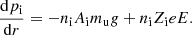
Following the arguments in Pelletier et al. (1986) and Paxton et al. (2018), we neglect thermal effects, and all terms involving collisions with electrons. The diffusion equations for a multicomponent plasma then take the form (Burgers 1969)
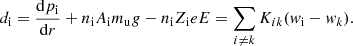
Here di is the driving force on ion i, provided by the partial pressure pi, the local gravity g, and electric field E. The atomic mass and charge units are mu and e, atomic mass Ai and average charge Zi, number density ni. The relative velocity between ions i and k is wi − wk, and Kik are the resistance coefficients, which are related in a simple way to the usual diffusion coefficients Dik (Pelletier et al. 1986).
In the case of diffusion equilibrium the relative velocities are zero, and the system of equations simplifies to a set of equations for the local abundance gradients,
For the electrons the gravitational term can be neglected:
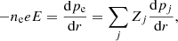
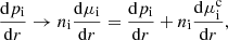
where the first equality comes from Eq. (10), and the second from the condition of electrical neutrality. This result serves to eliminate the electric field and leaves N linear equations for N ions.
These equations are derived and transformed under the assumption of a classical ideal gas EOS for electrons and ions. In the envelopes of white dwarfs two complications arise: the electrons may be partially degenerate, and Coulomb interactions in the plasma may not be negligible. We took the degeneracy into account by replacing

with the Boltzmann constant k and f determined from the Fermi-Dirac functions for partial degeneracy of the electrons.
For the consideration of non-ideal effects of the ions we follow Beznogov & Yakovlev (2013). They replace
where now pi is the ideal gas part as before, μi is the chemical potential of the ion, and  is the Coulomb interaction contribution. For the latter, they derive
with
At each depth in the envelope the system of equations for dpi/dr is solved and integrated alongside the three structure equation. This defines the abundance profiles ϵi(m).
As can be seen in the diffusion equations, we need the average charges of all ions Zi. In previous versions we used the approximation from Paquette et al. (1986; corrected for a missing factor of ρ1/3), which is based on the rather crude pressure ionization model of Fontaine & Michaud (1979). This model also assumes a trace element in a uniform background, which is not appropriate in our case, as shown below. New options are a Thomas-Fermi mean-ionization model (Stanton & Murillo 2016; More 1985), which is based originally on Feynman et al. (1949). This method elegantly takes into account the multicomponent nature of the plasma and is our preferred choice now. A third option are tables of mean charges for 20 elements from H to Ni, provided together with the Los Alamos opacity tables (Colgan et al. 2016).
3. Application to DQ white dwarfs
While individual results show some differences between the two recent studies of Koester & Kepler (2019) and Coutu et al. (2019), the important results agree and are discussed in the following. For these applications we used for the cool DQ the EOS of Saumon et al. (1995), if the abundances by number ϵ(H)+ϵ(He) > 0.999, and FreeEOS elsewhere. For the warm DQ, we used FreeEOS everywhere. The opacity was calculated from the OPAL tables for H, He, C, O mixtures. The average charges were determined with the Thomas-Fermi mean-ionization model.
3.1. Cool DQ
For the classical cool DQ with Swan bands, the main result is the appearance of a clearly defined sequence of objects from ∼10 000 K, [C/He] = −4.0 down to 5500 K and [C/He] = −7.0 (the notation [C/He] is used as abbreviation for abundances of log(n(C)/n(He))). Above this sequence other objects are scattered whose carbon abundances are up to 1 dex higher, possibly forming a second sequence. While these general results were already demonstrated in earlier work (Dufour et al. 2005; Koester & Knist 2006), the Gaia parallaxes now confirm that the DQ on the low abundance sequence (henceforth called only “the sequence”) have (almost) normal white dwarf masses.
Because the standard explanation for these cool DQ is dredge-up of carbon from the underlying He/C transition zone (Koester et al. 1982; Pelletier et al. 1986), the most natural parameter for the formation of the sequence is the thickness or total mass of the He layer. The latter study found that a relatively thin helium layer with q(He) in the range −3.5 to −4.0 provided the best fit to the observed carbon abundances. Improved calculations shown in Dufour et al. (2005) indicate a slightly higher range of −2.5 to −3.0, but it is still smaller than the predicted ≥−2.0 from evolutionary calculations.
While the cited papers used evolutionary calculations for white dwarfs including the effects of diffusion, in our current study we follow a complementary approach. At least the outer envelope at these low effective temperatures is certainly in diffusive equilibrium, therefore we integrate the envelope equations from the outside, with atmosphere models using observed abundances as starting point. The structure is followed inward through the convection zone (present in all DQ), where the matter is homogeneously mixed, and below, where the abundances change as described in the previous section. The integration is typically stopped at q = −2.0, or when the abundance fraction (by mass) of helium is below 10−4, whatever is deeper in the star.
Rather than using every observed DQ, we decided to describe the sequence with eight representative models. We divided the range from 9750 to 5750 K into 500 K wide intervals and determined average values for Teff, log g, and [C/He], excluding all objects with [C/He] greater than the average by more than 0.4 (to exclude the objects that lie clearly above the sequence). The parameters of the resulting model sequence are given in Table 1.
Parameters Teff, log g, [C/He], and standard deviation of the abundance distribution for eight models describing the observed sequence of cool DQ.
The log g averages in the intervals are close enough to the overall average 7.95, and we used this value for all models, varying only Teff and [C/He]. Atmospheric models were calculated with these parameters. Pressure and temperature at a deep layer (Rosseland τ = 90), together with radius, mass, and luminosity obtained from Teff and log g from the Montreal mass-radius relation2 were used as starting values for the envelope equations. Throughout the cvz, the abundances were held fixed at the atmospheric values; below the bottom they were changed according to the conditions of diffusive equilibrium. The resulting fractional masses in the cvz as well as the total fractional helium mass for different assumptions are given in Table 2. The different options are no overshoot, one pressure scale height overshoot below the formal bottom of the cvz, and a calculation without overshoot, but with the non-ideal term in the diffusion equations switched off.
Fractional mass in the convection zone q(cvz) = log Mcvz/M.
The 19 objects excluded from the determination of the model sequence because of higher C abundances have an average log g = 7.94, that is, their masses are identical with the cool sequence. We calculated additional atmosphere and envelope models for three parameter sets at the low and top end of the sequence and one in the middle with [C/He] increased by 1 dex compared to the standard. We also calculated three models with [C/He] decreased until the carbon features became undetectable, defined as a jump < 1% for the strong band head at 5163 Å (after convolving for the SDSS resolution). These six envelope models are presented in Table 3 and are compared with the standard sequence.
Envelope calculations for three representative models above the sequence with [C/He] enhanced by 1 dex, and with [C/He] decreased until the carbon features become undetectable in the SDSS spectra.
With our standard assumptions for the sequence (no overshoot, with non-ideal terms) we obtain helium layer masses that are slightly higher than in Pelletier et al. (1986), but lower than the more recent results in Dufour et al. (2005) or Coutu et al. (2019). We note, however, that these results depend strongly on the input physics used. When we include overshooting, the He mass increases by ∼0.4 dex, and when we neglect the non-ideal term in the diffusion equations, they increase by ∼0.9 dex (without overshooting!). Another ingredient that is very important for the depth of the cvz is the conductive opacity. Several scale heights above the bottom, the temperature gradient is already dominated by the conductive opacity, but it is still high enough to enforce convection. Thus the bottom of the cvz is determined by the decrease in conductive opacity.
The helium masses show a small systematic decrease in the lower part of the model sequence. Figure 12 in Coutu et al. (2019) also shows a slight deviation of the observed objects from a theoretical sequence with constant q(He), although the direction is different from our case: the coolest objects have higher He masses than the hotter ones, which contradicts our result. Nevertheless, the small change of ∼0.3 dex from warm to cool models is much smaller than the 2.5 dex span of carbon abundances observed at the surface. The explanation of the sequence as due to stars with very similar He masses is therefore probably correct, and small apparent trends are due to remaining imperfections of our models, especially at the cool end.
That the deepest convection zones (at 5900 K) lead to the lowest He masses disagrees with naive expectations. The main reason for this is the evolution of the average charge of carbon ions along the sequence from hot to cool Teff: at the bottom of the cvz, the temperature decreases, while the density increases, leading to a decrease of the average charge from 5.0 to 4.1. The gradients in the C/He transition zone become steeper and the total He mass decreases in spite of a slight increase in cvz mass. This change in average C charge is also the main reason for the huge decrease of carbon abundances along the sequence to the cool end. This is demonstrated in Fig. 1, which shows the number abundances of He and C in the envelopes as a function of effective temperature. While the total He content remains approximately constant, the gradients become much steeper with the decreasing average carbon charge, and the tail reached by the cvz accordingly has much lower C abundance. A similar effect has been noted before, and its importance was realized by Pelletier et al. (1986).
 |
Fig. 1. Number abundances for He and C in the lower part of the convection zone and below the bottom. The three panels show from top to bottom the models for Teff = 9335, 7503, and 5900 K. The curves give abundances for He (long red dashes, declining toward the interior on the left side) and C (continuous blue, declining toward the surface). The short-dashed curves in the middle panel result from switching off the non-ideal interactions in the diffusion equations, which results in a higher He mass by about a factor 10. The hatched area is the cvz. |
The effect of including the Coulomb interaction in the diffusion equations is demonstrated in the middle panel of Fig. 1, which shows the C/He abundance structure for the 7503 K model through the lower part of the cvz and in the region below. The interaction term leads to a steeper decline of the He abundance and thus to a lower total He mass fraction.
One reason for the small change in apparent He masses at low Teff could be an unseen hydrogen content in the DQ, which is not considered in our cool models. This has been discussed by Coutu et al. (2019), who concluded that the addition of [H/He] = −3.0 in the models does not significantly change the results. We find that even [H/He] = −4.0 would easily be detected and have used such a model grid for some test calculations. At the low Teff end (5900 K), the change of the model corresponds to a change in optical slope of ∼50 K hotter, and [C/He] higher by 0.1 dex. The flux at 4800 Å is about 0.05 mag higher, leading to a smaller radius estimate and an increase in log g by 0.05 dex. At higher Teff, the changes are smaller and completely negligible at the high Teff end. The same is true for the cvz depths and He masses (Table 4), which show only very minor differences to the models without hydrogen.
The additional models in Table 3 show that the cool DQ sequence spans only a rather narrow range of helium masses. A very small decrease leads to the few scattered objects above the sequence, while about 0.2 dex more renders the carbon features undetectable, and the objects would appear as featureless DC white dwarfs. This is of course influenced by observational bias. The white dwarf L 97-3 shows a completely featureless optical spectrum and was originally classified as a DC, until Koester et al. (1982) found strong C I lines in the ultraviolet region and determined an abundance of [C/He] = −6.0. Using the same methods as for the DQ, we find a fractional helium mass q(He) = −2.99, only 0.3 dex higher than would make the object a DQ in the visible region as well. This suggests a narrow distribution of He masses from stellar evolution, with the classical DQ formed by the low-mass tail and the majority of objects evolving as DC. Whether a continuous distribution can lead to such a sharply defined sequence, or if some special feature in this function is needed remains to be tested by stellar evolution calculations and population synthesis simulations. In this context, it will also be important to confirm (or refute) the apparent slight difference of 0.05 M⊙ between the average DQ and DC masses (Koester & Kepler 2019; Coutu et al. 2019).
3.2. Warm DQ
Warm DQ is the designation given to a group of carbon-rich white dwarfs at temperatures between ∼10 000 − 17 000 K, whose spectra are dominated by atomic lines of neutral carbon (C I). The new Gaia parallaxes have shown for the first time that all these stars have extremely high surface gravities above 8.50, corresponding to masses > 0.9 M⊙ (Koester & Kepler 2019; Coutu et al. 2019). In their analysis, Koester & Kepler (2019) noted that many of these objects showed hydrogen Balmer lines, but they kept the abundance fixed at [H/He] = −3.5, referring further analysis to the current study.
Our sample consists of 26 warm DQ with parameters Teff, log g, [C/He] given in the earlier study. These were the starting point for our determination of a more accurate H content. We realized, however, that a changed H content and closer inspection of the spectra demanded some changes in the parameters. In the range of 9300−11 000 K, weak C I lines, which had a negligible influence on the χ2 fitting, sometimes demanded a slightly higher Teff because they were too weak in the models. We therefore increased the temperature (and log g as demanded by the parallax) until the fit was more satisfactory. We note that this is not a final high-accuracy analysis because our interest is only to obtain reasonably accurate starting models for the envelope integration.
A more serious problem is presented by the helium-to-carbon ratio at temperatures > 11 500 K, with [C/He] > −2.0. The [C/He] ratio obtained by the χ2 fitting often produces a small but visible He I line 5877 Å, which is not observed in any of the warm DQ we analyzed. This is also true when we use the parameters of the common objects from Coutu et al. (2019) with our own models. When we increased the [C/He] ratio until this line became compatible with observations, in most cases we realized that the complete C I spectrum does not change with further increase, that is, the He abundance can only be regarded as an upper limit. This is unexpected because the χ2 fitting clearly leads to a solution with significant He contribution, but it might be explained with the extremely unsatisfactory status of the atomic data for neutral carbon in the optical range (Koester & Kepler 2019). For the lower Teff range and [He/C] > 2.0 there is still a small dependency of the carbon features on the abundance ratio, and we kept these results as measurement; some doubt remains whether these might in reality be just upper limits as well.
Carbon is always observed, whereas helium is not directly observed in any of the objects. We therefore preferred to change our abundance notation to using carbon as standard, and measuring He and H relative to C. The final parameters used for the 26 objects are given in Table 5, which also has the results for the depth of the convection zone and total H and He masses (which in the latter case are mostly upper limits). Figure 2 shows the atmospheric H and He abundances and upper limits for the whole range of temperatures. The cvz depths and H and He mass fractions are displayed in Fig. 3. A typical example (SDSSJ023633.74+250348.9) for the abundance structure in the envelope is provided in Fig. 4.
 |
Fig. 2. Atmospheric [H/C] and [He/C] abundance ratios and upper limits for warm DQ white dwarfs. Upper part (red): [He/C], and lower part (blue): [H/C]. The horizontal dashed line is the zero-point [He/C] = [H/C] = 0. |
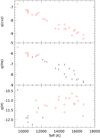 |
Fig. 3. Logarithmic fractional convection zone masses, helium, and hydrogen masses (red circles) and upper limits (black) for warm DQ. |
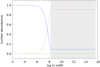 |
Fig. 4. Abundance structure of H (green, lowest curve), He (red, dashed), and C (blue, continuous) in SDSSJ0236+2503. On this linear scale the H abundance cannot be distinguished from zero. The hatched area is the convection zone. |
Atmospheric parameters Teff, log g (cgs units), [H/C], and [He/C] for 26 warm DQ white dwarfs.
Figure 3 shows that the mass in the cvz decreases with increasing Teff. If the cooler and warmer objects were evolutionary related, we would expect the atmospheric He abundance to decrease with cooling because the cvz becomes more massive. The opposite seems to happen – the He abundances are apparently higher at the low Teff end. We recall, however, that most if not all of the He abundances are upper limits, and the trend in the abundances at least partly reflects the increasing visibility of the He lines.
3.3. The puzzle of surface gravities
The studies of Koester & Kepler (2019) and Coutu et al. (2019) both reported a clear correlation of the surface gravity with temperature from 10 000−17 000 K that reached very high values at the hot end (Fig. 5, top panel). Both studies failed to identify shortcomings in the models (completely independent codes). This does not rule out that shortcomings can be found eventually because some arguments cast doubt on this Teff–log g correlation.
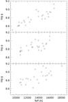 |
Fig. 5. Surface gravities as function of Teff. Top panel: standard results, with [He/C], Teff, and log g as variables. Middle panel: [H/C] = −2.0 and [He/C] = −1.50 fixed, only photometry is used to determine Teff and log g. Bottom panel: results after iterating between log g from photometry and Teff from spectra, with [H/C] and [He/C] fixed as above. |
First of all, we note that while the surface gravities in Table 5 extend over more than a factor of four, the spread in masses is only 0.28 M⊙ or about 26%, with a strong clustering between 1.05 and 1.16 M⊙. Because of the shape of the mass-radius relation at the high-mass end, a small change in mass leads to a much larger change of surface gravity. Another argument is given by the radial velocities. All objects show high redshifts ≥100 km s−1, with an average of 128 and a standard deviation of 38 km s−1, and no correlation with Teff. We assume that the standard deviation is caused by the space motion, which is not unrealistic because the median of the transverse velocity is ∼50 km s−1 (Coutu et al. 2019). The average gravitational redshift is then 128 km s−1, which at 13 000 K corresponds to a surface gravity of 8.98 and a mass of 1.17 M⊙. This is higher than the average mass from log g (1.07 M⊙), which might in part be caused by the strongly nonlinear relation between mass and gravitational redshift. This number might also indicate the result of the merger of two white dwarfs with the most likely masses of ∼0.58 M⊙.
Our result that most of the [He/C] results should be regarded as upper limits, as well the recent detection of a DAQ near Teff = 11 000 K with very unusual abundances (Hollands et al., in prep.), encouraged us to make a rather radical experiment. We used a model grid with [He/C] fixed at −1.50, which means that its influence on the spectra is negligible, and [H/C] fixed at −2.0, a typically observed value. The results for the surface gravities are shown in Fig. 5. One uses only photometry, and the other iterates between photometry for log g and spectroscopy for Teff. The standard results are included as well. The scatter in the two lower panels is larger than in the top, most likely because only two parameters are free in the fitting procedure. Nevertheless, the trend toward higher masses at higher temperatures is still apparent and seems to be a robust result, independent of the details of the analysis.
4. Discussion and conclusions
The total helium masses we find, even with overshooting included, are lower than predicted from stellar evolution. In their study of the full evolution from the main sequence to white dwarfs, including element diffusion, Althaus et al. (2009) and Miller Bertolami & Althaus (2006) found (log) He mass fractions of −1.99 for a white dwarf with 0.584 M⊙, with a range of −1.88 to −2.59 for white dwarf masses between 0.542 and 0.741 M⊙. Romero et al. (2013) calculated the complete evolution leading to ZZ Ceti variables, that is, DA with outer hydrogen envelope. They also presented numbers for the resulting He layer mass, which is −1.62 for a DA mass of 0.593 M⊙. Romero et al. (2012) argued that the He mass might decrease by a factor of four at most, when they enforced a large number of thermal pulses on the giant branch. However, in that case, the white dwarf mass increases to ∼0.7 M⊙.
Such He masses will lead to a pure He atmosphere and a white dwarf classified as DC (featureless spectrum) below 10 000 K effective temperature, or a DZ, if traces of metals other than C are present. Kepler et al. (2019) listed 2445 DC+DZ in the SDSS Data Release 14, and only 524 DQ. While this is certainly not a statistically valid sample, the analysis of Giammichele et al. (2012) of the white dwarfs within 20 pc lists about twice as many DZ+DC as DQ. The cool DQ are obviously not the majority among cool He-rich white dwarfs, but a significant fraction. It is therefore very likely that the relation between white dwarf (or progenitor) mass and final He layer mass is not strictly a one-to-one relation, but has some statistical element, perhaps with the exact number of thermal pulses experienced. The cool DQ then would originate from the lower tail of resulting helium masses.
The situation is far more complex for the warm DQs. Whether the He and H masses are real determinations or only upper limits, they are clearly much lower than would be expected from normal single-star evolution. As there is also no known single star progenitor population with this mass distribution, the currently favored explanation is that these massive objects are the results of the merger of two white dwarfs, as first proposed by Dunlap & Clemens (2015) for the hot DQ. Coutu et al. (2019) extended this to the warm DQ, which are considered to be the cooled-down descendants. For the hot DQ the argument rests on the discrepancy between the transversal velocities, which are characteristic for an older population, and the younger cooling age. Cheng et al. (2019) also concluded based on kinematic arguments that ∼20% of all white dwarfs in the range 0.8−1.3 M⊙ are the product of double white dwarf mergers. Their objects are, however, mostly hotter than 16 000 K, and the argument is less convincing for the warm DQ because of the longer cooling ages even for single stars. This leaves the high masses as the single argument. Many authors have studied the merger of two white dwarfs, but the emphasis usually is on the origin of supernova Ia events, and thus on the merger of high-mass white dwarfs with a total mass above the Chandrasekhar mass. Sato et al. (2015) also reported lower mass mergers, with individual stars of 0.5 and 0.6 M⊙, where the outcome is not an explosion but a massive white dwarf. All these mergers apparently go through a phase of spiral-in with a massive disk, and it seems plausible that such an evolution can remove almost the complete outer H and He layers, leaving such small amounts as we find in the warm DQ. To our knowledge, no detailed computations of the outer layers exist, however.
A major remaining problem is the apparent trend between log g and Teff, which seems to indicate that there is no evolutionary connection between the very massive objects near 16 000 K and the less massive ones below 13 000 K (which are still more massive than the cool DQ). Another argument is the increase in He abundance and also He masses with decreasing Teff, although this has to assume that the atmospheric He abundances are real and not upper limits. If this is confirmed, it would be highly unlikely that these two puzzles are unrelated, possibly suggesting a major shortcoming of current model atmospheres.
Coutu et al. (2019) proposed explaining the mass–Teff correlation as a pile-up of objects due to a slow-down of the cooling because of the interior crystallization and its dependence on stellar mass. Their Fig. 17 is somewhat deceiving, however, because the shown isochrones correspond to differences in logarithmic age. Using the Montreal single-star evolution calculations, we find that the cooling age of a DQ with 1.05 M⊙ is 0.38 Gy from 16 000−13 000 K, but 0.92 Gy from 13 000 to 10 000 Gy, yet there are far fewer objects in the second interval than in the first. It is also unknown whether the isochrones have any relevance if the sample of warm DQ does not constitute a cooling sequence. To compare with theoretical models, calculations are required that include binary interaction, as in Istrate et al. (2016).
The final question is where the cooled-down warm DQ are. They cannot avoid this fate, but there are very few if any DQ below 9500 K with masses above 0.8 M⊙. Koester & Kepler (2019) have suggested, although with rather questionable arguments, that the so-called peculiar DQ (DQpec) with shifted Swan bands might be descendants of the warm DQ. Blouin & Dufour (2019) have refuted this and found normal masses for the DQpec as well. In their interpretation, a DQ turns into a DQpec when the photospheric density exceeds 0.15 g cm−3, which occurs when they cool down to below 6500 K (depending also on carbon abundance). Six DQpec above this line are suggested to be probably magnetic. The results strongly depend on the temperature determinations: if they were higher, the surface gravities would also be higher. While the theoretical models of Blouin & Dufour (2019) and Blouin et al. (2019) represent the best currently possible effort, they still have to use uncertain approximations. The calculations by Kowalski (2010) of the density shift of the Swan bands show a rather large effect; Blouin et al. (2019) recalibrated the shift by an empirical factor of eight so that it agreed with the observed shifts. We completely agree with the statement by Blouin & Dufour (2019) that “more efforts on both the observational and theoretical fronts are needed to clarify the nature of these objects”.
On the observational fronts, spectra with high resolution and high signal-to-noise of warm DQ in the range 11 000−13 000 K could help to detect tiny He lines. Perhaps it would be even easier to perform UV observations of the region 1900−3500 Å, where large differences between helium-rich and helium-poor models are expected.
Acknowledgments
This work was financed in part by the Coordenação de Aperfeiçoamento de Pessoal de Nível Superior – Brasil (CAPES) – Finance Code 001, Conselho Nacional de Desenvolvimento Científico e Tecnológico – Brasil (CNPq), and Fundação de Amparo à Pesquisa do Rio Grande do Sul (FAPERGS) – Brasil. This research has made use of public data from the Sloan Digital Sky Survey and the Gaia Mission.
References
- Abolfathi, B., Aguado, D. S., Aguilar, G., et al. 2018, ApJS, 235, 42 [NASA ADS] [CrossRef] [Google Scholar]
- Althaus, L. G., Panei, J. A., Miller Bertolami, M. M., et al. 2009, ApJ, 704, 1605 [NASA ADS] [CrossRef] [Google Scholar]
- Beznogov, M. V., & Yakovlev, D. G. 2013, Phys. Rev. E, 111, 161101 [Google Scholar]
- Blouin, S., & Dufour, P. 2019, MNRAS, 490, 4166 [NASA ADS] [CrossRef] [Google Scholar]
- Blouin, S., Dufour, P., Thibeault, C., & Allard, N. F. 2019, ApJ, 878, 63 [NASA ADS] [CrossRef] [Google Scholar]
- Burgers, J. M. 1969, Flow Equations for Composite Gases (New York: Academic Press) [Google Scholar]
- Cassisi, S., Salaris, M., & Irwin, A. W. 2003, ApJ, 588, 862 [NASA ADS] [CrossRef] [Google Scholar]
- Cheng, S., Cummings, J. D., Ménard, B., & Toonen, S. 2019, ApJ, submitted [arXiv:1910.09558] [Google Scholar]
- Colgan, J., Kilcrease, D. P., Magee, N. H., et al. 2016, ApJ, 817, 116 [NASA ADS] [CrossRef] [Google Scholar]
- Coutu, S., Dufour, P., Bergeron, P., et al. 2019, ApJ, 885, 74 [NASA ADS] [CrossRef] [Google Scholar]
- Dufour, P., Bergeron, P., & Fontaine, G. 2005, ApJ, 627, 404 [NASA ADS] [CrossRef] [Google Scholar]
- Dunlap, B. H., & Clemens, J. C. 2015, in 19th European Workshop on White Dwarfs, eds. P. Dufour, P. Bergeron, & G. Fontaine, ASP Conf. Ser., 493, 547 [NASA ADS] [Google Scholar]
- Feynman, R. P., Metropolis, N., & Teller, E. 1949, Phys. Rev., 75, 1561 [NASA ADS] [CrossRef] [MathSciNet] [Google Scholar]
- Fontaine, G., & Michaud, G. 1979, ApJ, 231, 826 [NASA ADS] [CrossRef] [Google Scholar]
- Gaia Collaboration (Brown, A. G. A., et al.) 2018, A&A, 616, A1 [NASA ADS] [CrossRef] [EDP Sciences] [Google Scholar]
- Giammichele, N., Bergeron, P., & Dufour, P. 2012, ApJS, 199, 29 [NASA ADS] [CrossRef] [Google Scholar]
- Iglesias, C. A., & Rogers, F. J. 1996, ApJ, 464, 943 [NASA ADS] [CrossRef] [Google Scholar]
- Irwin, A. W. 2012, Astrophysics Source Code Library [record ascl:1211.002] [Google Scholar]
- Istrate, A. G., Marchant, P., Tauris, T. M., et al. 2016, A&A, 595, A35 [NASA ADS] [CrossRef] [EDP Sciences] [Google Scholar]
- Kepler, S. O., Pelisoli, I., Koester, D., et al. 2019, MNRAS, 486, 2169 [NASA ADS] [Google Scholar]
- Koester, D. 2009, A&A, 498, 517 [NASA ADS] [CrossRef] [EDP Sciences] [Google Scholar]
- Koester, D., & Kepler, S. O. 2019, A&A, 628, A102 [NASA ADS] [CrossRef] [EDP Sciences] [Google Scholar]
- Koester, D., & Knist, S. 2006, A&A, 454, 951 [NASA ADS] [CrossRef] [EDP Sciences] [Google Scholar]
- Koester, D., Weidemann, V., & Zeidler, E.-M. 1982, A&A, 116, 147 [NASA ADS] [Google Scholar]
- Kowalski, P. M. 2010, A&A, 519, L8 [NASA ADS] [CrossRef] [EDP Sciences] [Google Scholar]
- Miller Bertolami, M. M., & Althaus, L. G. 2006, A&A, 454, 845 [NASA ADS] [CrossRef] [EDP Sciences] [Google Scholar]
- More, R. M. 1985, Adv. At. Mol. Phys., 21, 305 [NASA ADS] [CrossRef] [Google Scholar]
- Paquette, C., Pelletier, C., Fontaine, G., & Michaud, G. 1986, ApJS, 61, 197 [NASA ADS] [CrossRef] [Google Scholar]
- Paxton, B., Schwab, J., Bauer, E. B., et al. 2018, ApJS, 234, 34 [NASA ADS] [CrossRef] [EDP Sciences] [Google Scholar]
- Pelletier, C., Fontaine, G., Wesemael, F., Michaud, G., & Wegner, G. 1986, ApJ, 307, 242 [NASA ADS] [CrossRef] [Google Scholar]
- Potekhin, A. Y., Baiko, D. A., Haensel, P., & Yakovlev, D. G. 1999, A&A, 346, 345 [NASA ADS] [Google Scholar]
- Potekhin, A. Y., Pons, J. A., & Page, D. 2015, Space Sci. Rev., 191, 239 [NASA ADS] [CrossRef] [Google Scholar]
- Press, W. H., Teukolsky, S. A., Vetterling, W. T., & Flannery, B. P. 1992, Numerical Recipes in FORTRAN. The Art of Scientific Computing, 2nd edn. (Cambridge: Cambridge University Press) [Google Scholar]
- Romero, A. D., Córsico, A. H., Althaus, L. G., et al. 2012, MNRAS, 420, 1462 [Google Scholar]
- Romero, A. D., Kepler, S. O., Córsico, A. H., Althaus, L. G., & Fraga, L. 2013, ApJ, 779, 58 [NASA ADS] [CrossRef] [Google Scholar]
- Sato, Y., Nakasato, N., Tanikawa, A., et al. 2015, ApJ, 807, 105 [NASA ADS] [CrossRef] [Google Scholar]
- Saumon, D., Chabrier, G., & van Horn, H. M. 1995, ApJS, 99, 713 [NASA ADS] [CrossRef] [Google Scholar]
- Stanton, L. G., & Murillo, M. S. 2016, Phys. Rev. E, 93, 043203 [NASA ADS] [CrossRef] [Google Scholar]
- Tassoul, M., Fontaine, G., & Winget, D. E. 1990, ApJS, 72, 335 [Google Scholar]
- York, D. G., Adelman, J., Anderson, Jr., J. E., et al. 2000, AJ, 120, 1579 [CrossRef] [Google Scholar]
All Tables
Parameters Teff, log g, [C/He], and standard deviation of the abundance distribution for eight models describing the observed sequence of cool DQ.
Envelope calculations for three representative models above the sequence with [C/He] enhanced by 1 dex, and with [C/He] decreased until the carbon features become undetectable in the SDSS spectra.
Atmospheric parameters Teff, log g (cgs units), [H/C], and [He/C] for 26 warm DQ white dwarfs.
All Figures
|
Fig. 1. Number abundances for He and C in the lower part of the convection zone and below the bottom. The three panels show from top to bottom the models for Teff = 9335, 7503, and 5900 K. The curves give abundances for He (long red dashes, declining toward the interior on the left side) and C (continuous blue, declining toward the surface). The short-dashed curves in the middle panel result from switching off the non-ideal interactions in the diffusion equations, which results in a higher He mass by about a factor 10. The hatched area is the cvz. |
| In the text | |
|
Fig. 2. Atmospheric [H/C] and [He/C] abundance ratios and upper limits for warm DQ white dwarfs. Upper part (red): [He/C], and lower part (blue): [H/C]. The horizontal dashed line is the zero-point [He/C] = [H/C] = 0. |
| In the text | |
|
Fig. 3. Logarithmic fractional convection zone masses, helium, and hydrogen masses (red circles) and upper limits (black) for warm DQ. |
| In the text | |
|
Fig. 4. Abundance structure of H (green, lowest curve), He (red, dashed), and C (blue, continuous) in SDSSJ0236+2503. On this linear scale the H abundance cannot be distinguished from zero. The hatched area is the convection zone. |
| In the text | |
|
Fig. 5. Surface gravities as function of Teff. Top panel: standard results, with [He/C], Teff, and log g as variables. Middle panel: [H/C] = −2.0 and [He/C] = −1.50 fixed, only photometry is used to determine Teff and log g. Bottom panel: results after iterating between log g from photometry and Teff from spectra, with [H/C] and [He/C] fixed as above. |
| In the text | |
Current usage metrics show cumulative count of Article Views (full-text article views including HTML views, PDF and ePub downloads, according to the available data) and Abstracts Views on Vision4Press platform.
Data correspond to usage on the plateform after 2015. The current usage metrics is available 48-96 hours after online publication and is updated daily on week days.
Initial download of the metrics may take a while.