| Issue |
A&A
Volume 635, March 2020
|
|
|---|---|---|
| Article Number | A147 | |
| Number of page(s) | 17 | |
| Section | Numerical methods and codes | |
| DOI | https://doi.org/10.1051/0004-6361/201937424 | |
| Published online | 24 March 2020 | |
Probabilistic direction-dependent ionospheric calibration for LOFAR-HBA
1
Leiden Observatory, Leiden University, PO Box 9513, 2300 Leiden, The Netherlands
e-mail: This email address is being protected from spambots. You need JavaScript enabled to view it.
2
International Centre for Radio Astronomy Research – Curtin University, GPO Box U1987, Perth, WA 6845, Australia
Received:
27
December
2019
Accepted:
31
January
2020
Abstract
Direction-dependent calibration and imaging is a vital part of producing radio images that are deep and have a high fidelity and highly dynamic range with a wide-field low-frequency array such as LOFAR. Currently, dedicated facet-based direction-dependent calibration algorithms rely on the assumption that the size of the isoplanatic patch is much larger than the separation between bright in-field calibrators. This assumption is often violated owing to the dynamic nature of the ionosphere, and as a result, direction-dependent errors affect image quality between calibrators. In this paper we propose a probabilistic physics-informed model for inferring ionospheric phase screens, providing a calibration for all sources in the field of view. We apply our method to a randomly selected observation from the LOFAR Two-Metre Sky Survey archive, and show that almost all direction-dependent effects between bright calibrators are corrected and that the root-mean-squared residuals around bright sources are reduced by 32% on average.
Key words: methods: data analysis / techniques: interferometric
© J. G. Albert et al. 2020
 Open Access article, published by EDP Sciences, under the terms of the Creative Commons Attribution License (https://creativecommons.org/licenses/by/4.0), which permits unrestricted use, distribution, and reproduction in any medium, provided the original work is properly cited.
1. Introduction
In radio astronomy many of the greatest questions can only be answered by observing the faintest emission over a large fraction of the sky surface area. Such large puzzles include searching for the epoch of reionisation (e.g. Patil et al. 2017), potentially detecting the missing baryons in the synchrotron cosmic web (e.g. Vernstrom et al. 2017), understanding the dynamics of galaxy cluster mergers (e.g. van Weeren et al. 2019), and probing matter distribution with weak gravitational lensing at radio frequencies (e.g. Harrison et al. 2016). In recent years, instruments such as the Low-Frequency Array (LOFAR; van Haarlem et al. 2013), the Murchison Widefield Array (MWA), and the future Square Kilometre Array (SKA) have been designed with the hope of discovering these key pieces in our understanding of the Universe. In particular, the prime objective of LOFAR, a mid-latitude array (N52°), is to be a sensitive, wide-field, wide-band surveying instrument of the entire northern hemisphere at low frequencies, although it is important to note that LOFAR effectively enables a host of other scientific goals such as real-time monitoring of the northern sky at low frequencies (Prasad et al. 2016).
While these instruments take decades to plan and build, arguably most of the technological difficulty follows after the instrument comes online as scientists come to understand the instruments. Even though LOFAR came online in 2012, after six years of construction, it was not until 2016 that a suitable direction-dependent (DD) calibrated image was produced for its high-band antennae (HBA; 115–189 MHz) (van Weeren et al. 2016), and although there has been much progress, there is currently still no DD calibrated image produced for its low-band antennae (LBA; 42–66 MHz). Importantly, despite many years in developing these initial DD calibration and imaging algorithms, they were not suitable for the primary survey objective of LOFAR. Thus, there has been continuous work aimed at improving them.
The main cause of DD effects in radio interferometry is the ionosphere. The ionosphere is a turbulent, low-density, multi-species ion plasma encompassing the Earth, driven mainly by solar extreme ultra-violet radiation (Kivelson & Russell 1995) that changes on the timescale of tens of seconds (Phillips 1952). The free electron density (FED) of the ionosphere gives rise to a spatially and temporally varying refractive index at radio wavelengths. This causes weak scattering of electric fields passing through the ionosphere (Ratcliffe 1956), which becomes more severe at lower frequencies, and results in the scattering of radio radiation onto radio interferometers. Despite the weak-scattering conditions, the integral effect of repeated scattering through the thick ionosphere can cause dispersive phase variations of well over 1 radian on the ground (Hewish 1951, 1952).
Wide-field radio arrays, such as LOFAR, are particularly susceptible to the DD effects of the ionosphere (Cohen & Röttgering 2009) because the field of view is many isoplanatic patches (Fellgett & Linfoot 1955) wherein the instantaneous scattering properties of the ionosphere change significantly over the field of view. In order to achieve the science goals in the wide-field regime, a DD calibration strategy must be adopted (Cornwell et al. 2005). Many DD approaches have been developed, ranging from field-based calibration (Cotton et al. 2004) and expectation-maximisation (Kazemi et al. 2011) to facet-based approaches (Intema et al. 2009; van Weeren et al. 2016; Tasse et al. 2018).
Common to all of these DD techniques is the requirement that the signal-to-noise ratio needs to be high enough on short enough time intervals where the ionosphere can be considered fixed. Therefore, bright compact sources are required throughout the field of view, which act as in-field calibrators. The fundamental assumption is that the distance between calibrators is less than the isoplanatic-patch size, which is about 1° for nominal ionospheric conditions. However, this quantity is dynamic over the course of an observation, and this assumption can be broken at times.
With the advent of the killMS DD calibration algorithm (Tasse 2014a; Smirnov & Tasse 2015), and the DDFacet DD imager (Tasse et al. 2018), the LOFAR Two-Metre Sky Survey (LoTSS; Shimwell et al. 2017) became possible, and the LoTSS first data release (DR1) has become available (Shimwell et al. 2019). While LoTSS-DR1 provides an excellent median sensitivity of S144 MHz = 71 μJy beam−1 and point-source completeness of 90%, there are still significant DD effects in the images between the in-field calibrators. Improving the DD calibration for LoTSS is therefore a priority.
The second data release (DR2) is preliminarily described in Shimwell et al. (2019), and will be fully described in Tasse et al. (in prep.). Because we have internal access to this archive, we make reference to LoTSS-DR2.
The aim of this work is to present a solution to this limitation by probabilistically inferring the DD calibrations for all sources in a field of view based on information of the DD calibrations for a sparse set of bright calibrators. Importantly, this approach can be treated as an add-on to the existing LoTSS calibration and imaging pipeline.
We arrange this paper as follows. In Sect. 2 we formally define the problem of the DD calibration of ionospheric effects through inference of the doubly differential total electron content. In Sect. 3 we describe the procedure we used to perform the DD calibration and imaging of a randomly chosen LoTSS-DR2 observation using doubly differential total electron content screens. In Sect. 4 we compare our image with the LoTSS-DR2 archival image.
2. Doubly differential phase screens
In radio interferometry the observable quantity is the collection of spatial auto-correlations of the electric field, which are called the visibilities. The relation between the electric field intensity and the visibilities is given by the radio interferometry measurement equation (RIME; Hamaker et al. 1996),
 (1)
(1)
where we have left out frequency dependence for visual clarity, although for future reference, we let there be Nfreq sub-bands of the bandwidth.
In order to understand Eq. (1), let the celestial radio sky be formed of a countably infinite number of discrete point sources with directions in 𝒦 = {ki ∈ 𝕊2 ∣ i = 1…Ndir}. The propagation of a monochromatic polarised celestial electric field E(k) can be described by the phenomenological Jones algebra (Jones 1941). Letting the locations of antennae be 𝒳 = {xi ∈ ℝ3 ∣ i = 1…Nant}, then E(x, k) = h(x, k)J(x, k)E(k) denotes propagation of E(k) to x through the optical pathway indexed by (x, k), where h(x, k) is the Huygens–Fresnel propagator in a vacuum. Each antenna has a known instrumental optical transfer function that gives rise to another Jones matrix known as the beam, B(x, k). The total electric field measured by an antenna at x is then E(x) = ∑k∈𝒦h(x, k)B(x, k)J(x, k)E(k), and Eq. (1) follows from considering the auto-correlation of the electric field between antennae and imposing the physical assumption that the celestial radiation is incoherent.
Some words on terminology: although h, B, and J are all Jones operators, we only refer to J as the Jones matrices going forward, and we index them with a tuple of antenna location and direction (x, k). This corresponds to an optical pathway. When a Jones matrix is a scalar times identity, the Jones matrix commutes as a scalar, and we simply use scalar notation. This is the case, for example, when the Jones matrices are polarisation independent. It is also common terminology to call the sky-brightness distribution, I(k) ≜ ⟨E(k)⊗E†(k)⟩, the image or sky model, and values of the sky-brightness distribution are components.
In radio astronomy we measure the visibilities and invert the RIME iteratively for the sky model and Jones matrices. The process is broken into two steps called calibration and imaging. In the calibration step the current estimate of the sky model is held constant and the Jones matrices are inferred. In the imaging step the current estimate of the Jones matrices are held constant and the sky model is inferred. In both the imaging and calibration steps the algorithm performing the inference can be either direction independent (DI) or DD, which stems from the type of approximation made on the RIME when the visibilities are modelled. Namely, the DI assumption states that the Jones matrices are the same for all directions, and the DD assumption states that the Jones matrices have some form of directional dependence.
In the current work we focus entirely on the Stokes-I, that is, polarisation independent, calibration and imaging program used by the LoTSS pipeline. The LoTSS calibration and imaging pipeline is broken up into a DI calibration and imaging step followed by a DD calibration and imaging step.
Equation (1) shows that each optical pathway (x, k) has its own unique Jones matrix J(x, k) describing the propagation of radiation. In total, this results in 2NdirNant degrees of freedom for  observables. In practice, during DD calibration and imaging, this is never assumed for three main reasons. Firstly, the computational memory requirements of giving every direction a Jones matrix are prohibitive. Secondly, because Ndir ≫ Nant it would allow too many degrees of freedom per observable, which leads to ill-conditioning. Thirdly, most sky-model components are too faint to infer a Jones matrix on the timescales that the ionosphere can be considered fixed.
The LoTSS calibration and imaging program manages to handle the computational memory requirement and ill-conditioning through a clever sparsification of the optimisation Jacobian and by invoking an extended Kalman filter, respectively; see Tasse (2014a,b), Smirnov & Tasse (2015) for details. However, there is no way to prevent the third issue of a too low signal on required timescales, and they are limited to tessellating the field of view into approximately Ncal ≈ 45 facets, defined by a set of calibrator directions, 𝒦cal ⊂ 𝒦. The result of DI and DD calibration and imaging for LoTSS is therefore a set of Nant DI Jones matrices, and a set of NcalNant DD Jones matrices.
We consider the functional form of the final Jones matrices following this two-part calibration and imaging program. For each (x, k)∈𝒳 × 𝒦cal we have the associated calibration Jones matrix,
 (2)
(2)
 (3)
(3)
where notation t ≜ m means definition by equality, and can be read as “t is equal by definition to m”. An effective direction can intuitively be defined for the DI Jones matrices as the direction, k′, that minimises the instantaneous image domain dispersive phase error effects in the DI image. Clearly, this leads to problems for a wide-field instrument, where the actual Jones matrices can vary considerably over the field of view. It is fairly simple to contrive examples where there is no well-defined effective direction. Nonetheless, we use this terminology and return to address the associated problems shortly.
From the Wiener–Khinchin theorem it follows that the visibilities are independent of the electric field phase, therefore a choice is made to spatially phase reference the Jones matrices to the location x0 of a reference antenna. Doing so defines the differential phase,
 (4)
(4)
Now, we consider a set of observed visibilities, which are perfectly described by Eq. (1), where we neglect time, frequency, or baseline averaging. Then, there must be a set of true Jones matrices, 𝒥true = {Jtrue(x, k) ∣ (x, k)∈𝒳 × 𝒦}, which give rise to the observed visibilities. We assume that this set of Jones matrices is unique. Because the Jones matrices are assumed to be scalars, we can write them as Jtrue(x, k)≜Jtrue(x, k)eiΔ0ϕtrue(x, k).
Next, we consider the process of inferring the true Jones scalars from the observed visibilities using piece-wise constant calibration Jones scalars, Jcal(x, k), as is done in killMS. To do so, we define the operation ⌊k⌋ = argmaxk′ ∈ 𝒦calk ⋅ k′ as the closest calibration direction to a given direction. In general, it is always be possible to write the true Jones scalars, Jtrue(x, k), in terms of the resulting calibration Jones scalars Jcal(x, k) as
 (5)
(5)
where α(x, k) and Δ0β(x, k) correspond to the correction factors that would need to be applied to each calibration Jones scalar to make it equal to the true Jones scalar along that optical pathway. We assume the situation where there is enough information in the observed visibilities to strongly constrain the calibration Jones scalars, and that we are able to point-wise solve for a global optimum. This is unique by our above assumption. Then, if the distance between calibrators is much less than the isoplanatic-patch size (Fellgett & Linfoot 1955), we have that α ≈ 1 and Δ0β ≈ 0.
The substance of this paper is aimed at inferring the function Δ0β for all optical pathways (we pay minor attention to α as well). Because of the dynamic nature of the ionosphere, the calibration facets are not always isoplanatic (k ≉ ⌊k⌋ in the appropriate sense defined in Fellgett & Linfoot 1955), and consequently, Δ0β ≉ 0 sometimes.
We now focus our attention on the calibration Jones matrices in the direction of the calibrators and consider the value of Δ0β(x, k) for (x, k)∈𝒳 × 𝒦cal. In the event that Δ0β(x, k) ≈ 0, then from Eqs. (3) and (5) it follows that the DD differential phases are
 (6)
(6)
This states that in the directions of the calibrators, the DD calibration Jones phases are equal to the difference between the true Jones phases and DI Jones phases. However, in a typical application of facet-based calibration, we can easily see that this statement is usually false. It basically means that the designation of DI and DD for the Jones matrices inferred in calibration and imaging is a misnomer.
Firstly, specifying that the DI Jones matrices have a single effective direction is an invalid statement. The effective direction, as defined above, minimises the instantaneous image domain dispersive phase error effects, and this depends largely on the ionosphere, geometry of the optical pathways, and the sky-brightness distribution. The ionosphere changes in time, acting as a time-varying scattering layer in the optical system, therefore the effective direction is also dynamic. The effective direction is heavily weighted towards the brightest sources in the field of view, and because longer baselines “see” less flux, the effective direction is different for each antenna. To a lesser extent, the sensitivity drop-off at lower frequencies also introduces an effective direction that changes with sub-band frequency. Secondly, although DI calibration should remove all DI components such as station clocks, in practice, there are always remnant DI components in the DD Jones matrices.
It is desirable to assume that Eq. (6) holds in going forward because we interpret this to mean that we can make Δ0β(x, k) ≈ 0 everywhere through an appropriate choice of Δ0ϕDD(x, k). Therefore, we consider how the DD calibration can be modified such that Eq. (6) holds.
We address the first issue above, of ill-defined effective direction, by suitably forcing the observed visibilities to be well-approximated by isolated calibrators. This is applied and discussed further in Sect. 3.1.
To correct the second issue, to exactly separate all DI components from the DD Jones matrices, we use a trick. In Eq. (1) we can factor all commutative DI factors out in front of the summation. As we show in Appendix A, this is equivalent to directionally phase-referencing the Jones scalars, which we denote as doubly differential phase,
 (7)
(7)
Moreover, we show that doubly differential phase is guaranteed to have no DI components. This trick is used and discussed further in Sect. 3.3.
After applying the above two fixes, Eq. (6) then takes the form of a doubly differential phase,  . These not only have no DI components, but also have a well-defined reference direction. Both attributes are vital for our modelling method.
Finally, this paper is concerned with performing DD calibration by inferring  for a set of isolated calibrators followed by interpolation of these values to a multitude of optical pathways, which we call a screen. We assume that the DD Jones scalars are dominated by ionospheric dispersive phase effects and slowly changing beam errors. We neglect the ionospheric amplitude effects in this description because the phase effects are far more dominant. When the frequency of radiation is far above the ionospheric plasma frequency, then the ionospheric phase effects are given by a dispersive phase. The dispersive phase retards the wavefront without distorting it. The doubly differential ionospheric dispersive phase is given by
 (8)
(8)
where  is doubly differential total electron content (DDTEC), and
  .
.
3. Methods
In this paper we push beyond the current state-of-the-art LoTSS DD calibration and imaging using a physics-informed probabilistic model to infer DDTEC screens. We perform our screen-based DD calibration and imaging on a randomly selected eight-hour observation from the LoTSS-DR2 archive. The selected observation, LoTSS-DR2 pointing P126+65, was observed between 23:12:14 on 8 December, 2016, and 07:28:34 on 9 December, 2016, during solar cycle 241. The ionosphere activity during this observation was mixed, with the first half of the observation “wild” (DDTEC exceeding 100 mTECU) and the last half “calm”.
We first provide an overview of the our DD calibration and imaging procedure, before providing a deeper explanation of each step. A summary of our DD calibration and imaging program can be seen in Fig. 1 and is as follows:
-
Subtract and solve step. Subtract a good model of the sky, except approximately 35 bright calibrators (peak flux > 0.3 Jy beam−1). Solve against isolated calibrators.
-
Smooth and slow-resolve. Smooth the Jones scalars, and resolve on a long timescale to simultaneously reduce the degrees of freedom and solve the hole problem (for a description of the problem, see Shimwell et al. 2019).
-
Measure DDTEC. Infer DDTEC from the Jones scalars in the directions of the bright calibrators.
-
Infer DDTEC screen. Apply our DDTEC model to infer DDTEC for all intermediate brightness optical pathways (>0.01 Jy beam−1), forming a screen over the field of view.
-
Image screen. Concatenate the smoothed solutions with the DDTEC screen. Image the original visibilities with this set of solutions.
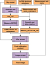 |
Fig. 1. Flow diagram overview of our DD calibration and imaging program. |
3.1. Subtract and solve
In this step we isolate a set of calibrators by subtracting the complementary sky model and then perform a solve. The process is visualised in the correspondingly labelled process box in Fig. 4.
We begin by selecting a set of bright calibrators (peak flux >0.3 Jy beam−1). The goal is to cover the field of view as uniformly as possible while not selecting too many calibrators, which can result in ill-conditioning of the system of equations that must be solved. In practice, we usually do not have enough bright calibrators to worry about ill-conditioning. Our selection criteria resulted in 36 calibrators whose layout is shown in Fig. 2 alongside the 45 calibrators selected by the LoTSS-DR2 pipeline.
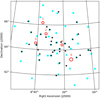 |
Fig. 2. Layout of our selected calibrators (black stars) compared to the LoTSS-DR2 archival calibrator layout (cyan circles). The calibrators define a facet tessellation of the field of view. The red circles indicate the regions of the cutouts in Fig. 10. |
As stated in Sect. 2, for our method to work, it is vital that the directions of the calibrators are well defined. The Jones matrix for each calibrator can be considered as a DI Jones matrix within the calibrator facet, therefore the notion of effective direction, as the direction that minimises instantaneous image domain artefacts, applies within a facet as well. Intuitively, the effective direction is located near the brightest sources in a facet. For example, in Fig. 3 the central source is by far brighter than all nearby sources, consequently, the dispersive errors in that direction are minimised. This defines an average effective direction.
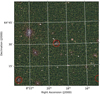 |
Fig. 3. Example of an average effective direction in a facet. The red circles indicate calibrators. The central calibrator has a peak flux of 0.91 Jy beam−1, while the next brightest non-calibrator source, approximately 16′ to the left, is 0.12 Jy beam−1. Within the facet of the calibrator, the Jones matrices are mostly optimised in a direction of the calibrator, but this effective direction changes over time, baseline, and frequency. |
Because the effective direction changes over time, baseline, and frequency, it follows that DD modelling is systematically biased by the unknown direction of the Jones matrices if they are based on these ill-defined effective directions. We circumvent this issue by first subtracting all sources from the visibilities, except for the bright calibrators. This requires having a good enough initial sky model. In our case we use the sky model from the LoTSS-DR2 archive. We mask a 120″ disc around each calibrator, ensuring that all artefacts for the calibrators are included in the mask. We predict the visibilities associated with the remainder of the sky model, pre-applying the solutions from the LoTSS-DR2 archive. We then subtract these predicted visibilities from the raw visibilities in the DATA column of the measurement set, placing the result in a DATA_SUBTRACT column of the measurement set. After they are subtracted, the isolated calibrator sources provide well-defined directions, which is crucial for Eq. (6) to hold.
We note that any unmodelled flux missing from the sky model will still reside in the visibilities, leading to a systematic calibration bias when the RIME is inverted. However, they will have been missing from the model due to their inherent faintness, therefore they should have minimal effect on the effective directions inside the facets of the isolated calibrators.
It is possible that a bright extended source be included in the set of calibrators. In this case, the model of the extended source is truncated at a radius of 120″ from the peak. Because the sky model is necessarily incomplete, residual flux of the extended source is left over. As above, because these residual components are faint, they have negligible effects on the resulting effective direction of the calibrator. Another problem of choosing extended sources as calibrators is that of convergence due to their resolved nature. Extended calibrators can lead to divergent calibration Jones scalars, which is a problem that must also be handled by any calibration and imaging program. In our case, the sky model comes from the LoTSS-DR2 archive, which provides a carefully self-calibrated model at the same frequency and resolution, and we expect to suffer less strongly from divergent solutions.
We perform a solve on DATA_SUBTRACT against the sky-model components of the isolated bright calibrators. We call these solutions raw_cal for future reference.
Several non-ionospheric systematics will be in raw_cal. Firstly, beam errors are a systematic that come from performing calibration with an incomplete beam model, as well as with an aperture array that contains dead or disturbed array tiles. The beam model can be improved by better physical modelling of the aperture array, which requires a complex solutions to Maxwell’s equations. The second issue is a transient effect because tiles can go dead over time and the dielectric properties of the antennae environment can change with temperature and air moisture content. It is important in the following to account for beam errors. Beam errors a priori are expected to change slowly over the course of an observation.
Another systematic that will find its way into the raw_cal are unmodelled sources outside the image, in LOFAR’s relatively high-sensitivity side-lobes. The effect of such unmodelled sources on calibration is still being understood. As noted in Shimwell et al. (2019), such sources can be absorbed by additional degrees of freedom during calibration. Because they are not within the imaged region, this flux absorption can go unnoticed. It is therefore important in the following to limit the degrees of freedom of the calibration Jones scalars.
3.2. Smooth and slow-resolve
There are enough degrees of freedom in a DD solve for unmodelled flux to be absorbed (Shimwell et al. 2019), therefore naively applying raw_cal and imaging would be detrimental to source completeness. Shimwell et al. (2019) found that a post-processing step of Jones scalar phase and amplitude smoothing removed enough degrees of smoothing to alleviate this problem. However, they then discovered that such a smoothing operation introduces negative halos around sources, the systematic origin of which has yet to be determined. A second solve on a much longer timescale alleviates the negative halo problem. The process is visualised in the correspondingly labelled process box in Fig. 4.
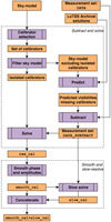 |
Fig. 4. Flow chart of the subtract and solve and smooth and slow-resolve steps. Together, they represent a DD calibration program similar to the LoTSS-DR1 and DR2 pipelines. |
The LoTSS DD calibration and imaging pipeline performs Jones scalar phase smoothing by fitting a TEC-like and constant-in-frequency functional form to the Jones phases using maximum likelihood estimation. This results in two parameters per 24 observables. We alter the smoothing method by fitting a three parameter model: a TEC-like term, a constant-in-frequency, and a clock-like functional form. Our choice results in three parameters per 24 observables. We add the additional term because a small (≲1 ns) remnant clock-like term appears to exist in the DD Jones phases.
Weak scattering in the ionosphere causes a well-known DD amplitude effect, however the amplitudes of the Jones scalars in raw_cal are more complicated, with possible contamination from an improperly modelled beam and unmodelled flux. Therefore, we do not consider modelling amplitude in this work, but we do impose the prior belief that beam error amplitudes change slowly over time and frequency as in Shimwell et al. (2019). To impose this prior, we simply smooth the log-amplitudes of raw_cal with a two-dimensional median filter in time and frequency with window size (15 min, 3.91 MHz).
Scintillation can also significantly effect the amplitudes of the Jones scalars. When the scintillation timescale is shorter than the integration timescale, the observed visibilities can decohere. In this case, the visibilities should be flagged. DDFacet contains an adaptive visibility weighting mechanism inspired by the optical method of “lucky imaging” that down-weights noisy visibilties (Bonnassieux et al. 2018), which effectively handles fast scintillation. When scintillation occurs on a longer timescale, the effect is characterised by amplitude jumps for groups of nearby antennae within the Fresnel zone. These effects are predominately removed during the DI calibration and are not considered further. This implies that we do not consider DD scintillation.
A surprising result of the smoothing procedure is that it introduces negative halos around bright sources, which destroys the integrity of the image. In the LoTSS pipeline, despite much effort to understand the fundamental cause of the problem, a temporary solution is to pre-apply the smoothed solutions and resolve against the same sky model on a long timescale. We perform this resolve with a solution interval of 45 min and call these solutions slow_cal. We form the concatenation of smooth_cal and slow_cal and call it smooth_cal+slow_cal.
3.3. Measure DDTEC
Next, we extract precise DDTEC measurements from raw_cal, which are later used to infer a DDTEC screen. While it would be possible to model a DDTEC screen directly on Jones scalars, the required inference algorithm would be extremely expensive to account for the high-dimensional, complicated, multi-modal posterior distribution that occurs due to phase wrapping. Therefore, in this section we describe how we use the ν−1 dependence of dispersive phase (Eq. (8)) to measure DDTEC2. The process is visualised in the correspondingly labelled box of Fig. 8.
First, we directionally reference the Jones phases in raw_cal by subtracting the phase of the brightest calibrator, that is, the reference calibrator, from the phases of all other directions. We can assume that all remnant DI effects are removed from the resulting doubly differential phases (see Appendix A). We then assume that these Jones scalar phases are completely described by DDTEC and the smoothed amplitudes coming from beam errors.
The idea of fitting frequency ν−1 dependence to phase to extract a TEC-like term is not new (e.g. van Weeren et al. 2016). However, fitting ionospheric components from Jones scalars is a notoriously difficult procedure because the Jones scalars are typically noise dominated, with heteroscedastic correlated noise profiles, and there are many local minima caused by phase-wrapping. Figure 5 shows an example of simulated Jones scalars data for a single optical pathway with a typical observational noise profile corresponding to a remote antenna and calibrator peak flux of 0.3 Jy beam−1. Typically, the problem is solved using maximum-likelihood estimators and the resulting TEC-like parameters are too biased or of high variance to be used for any sort of inference. For our purposes we require uncertainties of the measured DDTEC, which should be of the order of a few mTECU.
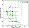 |
Fig. 5. Simulated real and imaginary components of noise-dominated Jones scalars and observational uncertainties. The simulated ground truth DDTEC is 150 mTECU and the observational uncertainties are frequency dependent and correlated, corresponding to a remote station for a calibrator at the cutoff peak flux limit of 0.3 Jy beam−1. |
We formulate the problem as a hidden Markov model (HHM; Rabiner & Juang 1986). In this HMM the Jones scalars of an optical pathway form a sequence of observables indexed by time, and the DDTEC of the optical pathway forms a Markov chain of hidden variables. We then apply recursive Bayesian estimation to obtain the posterior distribution of the DDTEC at each point in time given the entire Jones scalar sequence. As shown in Appendix B, this can be done in two passes over the data, using the forward and backward recursions, Eqs. (B.3) and (B.5), respectively.
Let gi ∈ ℂNfreq be the observed complex Jones scalar vector at time step i, and let  be the corresponding DDTEC. For visual clarity, we drop the optical pathway designation because this analysis happens per optical pathway.
We assume that the Jones scalars have Gaussian noise, described by the observational covariance matrix Σ. Thus, we define the likelihood of the Jones scalars as
![Mathematical equation: $$ \begin{aligned} p(\boldsymbol{g}_i \mid \Delta _0^2\tau _i, \boldsymbol{\Sigma }) = \mathcal{N} _\mathbb{C} [\boldsymbol{g}_i \mid |\tilde{\boldsymbol{g}}_i| \mathrm{e}^{i \frac{\kappa }{\nu } \Delta _0^2\tau _i}, \boldsymbol{\Sigma }], \end{aligned} $$](/articles/aa/full_html/2020/03/aa37424-19/aa37424-19-eq15.gif) (9)
(9)
where  denotes the smoothed amplitudes, and 𝒩ℂ denotes the complex Gaussian distribution. The complex Gaussian distribution of a complex random variable is formulated as a multivariate Gaussian of the stacked real and imaginary parts.
Because we expect spatial and temporal continuity of FED, the DDTEC should also exhibit this continuity. Therefore, we assume that in equal time intervals the DDTEC is a Lévy process with Gaussian steps,
![Mathematical equation: $$ \begin{aligned} p(\Delta _0^2\tau _{i+1} \mid \Delta _0^2\tau _i) = \mathcal{N} [\Delta _0^2\tau _{i+1} \mid \Delta _0^2\tau _i, \omega ^2 \delta t], \end{aligned} $$](/articles/aa/full_html/2020/03/aa37424-19/aa37424-19-eq17.gif) (10)
(10)
where ω2 is the variance of the step size. This is equivalent to saying that the DDTEC prior is a Gaussian random walk.
Equations (9) and (10) define the HMM data likelihood and state transition distribution necessary to compute Eqs. (B.3) and (B.5). The relation between DDTEC and amplitude and the Jones scalars is non-linear, therefore Eq. (B.3) is analytically intractable. To evaluate the forward equation, we apply variational inference, which is an approximate Bayesian method. Variational inference proceeds by approximating a distribution with a tractable so-called variational distribution with variational parameters that must be learned from data (e.g. Hensman et al. 2013). A lower bound on the Bayesian evidence is maximised for a point-wise estimate of the variational parameters, resulting in a variational distribution that closely resembles the actual distribution.
We assume that the variational forward distribution for DDTEC, at time step i given all past Jones scalars, g0:i, is closely approximated by a Gaussian,
![Mathematical equation: $$ \begin{aligned} q(\Delta _0^2\tau _{i}) = \mathcal{N} [\Delta _0^2\tau _{i} \mid m_{i}, \gamma ^2_{i}], \end{aligned} $$](/articles/aa/full_html/2020/03/aa37424-19/aa37424-19-eq18.gif) (11)
(11)
where the mean and variance is mi and  , respectively. When this choice is made, the state transition distribution is conjugate, and the forward recursion reduces to the well-known Kalman-filter equations, and the backward recursion reduces to the Rauch-smoother equations (Rauch 1963).
We consider marginalisation of the state transition distribution in Eq. (B.2). Marginalising with respect to Eq. (11) at time step i − 1, we obtain
![Mathematical equation: $$ \begin{aligned} p(\Delta _0^2\tau _i \mid \boldsymbol{g}_{0:i-1}, \boldsymbol{\Sigma }) = \mathcal{N} [\Delta _0^2\tau _i \mid m_{i-1}, \omega ^2 \delta t + \gamma ^{2}_{i-1}]. \end{aligned} $$](/articles/aa/full_html/2020/03/aa37424-19/aa37424-19-eq20.gif) (12)
(12)
This can be viewed as the propagated prior belief in DDTEC. The forward probability density is then given by Bayes equation,
 (13)
(13)
This is the posterior probability density given all previous observations in the observable sequence.
Variational inference proceeds by minimising the Kullbeck-Leibler divergence KL[q ∥ p] = ∫ℝ log q/p dq from the variational forward distribution q to the true forward distribution p with respect to the variational parameters. Equivalently, we may maximise the following evidence lower-bound objective (ELBO),
![Mathematical equation: $$ \begin{aligned} \mathcal{L} _i[q,p]&= \mathbb{E} _{q(\Delta _0^2\tau _{i-1})}\left[\log \frac{{p}(\Delta _0^2\tau _{i} \mid \boldsymbol{g}_{0:i}, \boldsymbol{\Sigma }) p(\Delta _0^2\tau _i \mid \boldsymbol{g}_{0:i-1}, \boldsymbol{\Sigma })}{q(\Delta _0^2\tau _{i-1})}\right] \\&= \mathbb{E} _{q(\Delta _0^2\tau _{i-1})}\left[\log p(\boldsymbol{g}_i \mid \Delta _0^2\tau _i, \boldsymbol{\Sigma }) \right] \end{aligned} $$](/articles/aa/full_html/2020/03/aa37424-19/aa37424-19-eq22.gif) (14)
(14)
![Mathematical equation: $$ \quad - \mathrm{KL} [q(\Delta _0^2\tau _{i-1}) \mid \mid p(\Delta _0^2\tau _i \mid \boldsymbol{g}_{0:i-1}, \boldsymbol{\Sigma })].$$](/articles/aa/full_html/2020/03/aa37424-19/aa37424-19-eq23.gif) (15)
(15)
Because the variational and prior distributions are both Gaussian, there is an analytic expression for the KL term3. The expectation of the likelihood term is called the variational expectation and is analytically derived in Appendix C.
One of the benefits of variational inference is that it turns a problem that requires computationally expensive Markov chain Monte Carlo methods into an inexpensive optimisation problem. It works well so long as the variational distribution adequately describes the true distribution.
We have assumed the variational forward distribution to be Gaussian, therefore the approximated system becomes a linear dynamical system (LDS). Several great properties follow. Firstly, the backward equation, Eq. (B.5), is reduced to the Rauch recurrence relations (Rauch 1963), which are easily accessible (e.g. Shumway & Stoffer 1982), so we do not write them down here. The Rauch recurrence relations are analytically tractable. As long as the variational forward distribution is a reasonable approximation, they therefore provide a computationally inexpensive improvement to DDTEC estimation. In contrast, performing the forward filtering problem alone uses only half of the available information in the observable sequence.
Secondly, the unknown step size variance ω and the observational uncertainty Σ can be estimated iteratively using the expectation-maximisation (EM) algorithm for LDS (Shumway & Stoffer 1982). For a good introduction to HHMs and parameter estimation see Shumway & Stoffer (1982), Rabiner & Juang (1986), and Dean et al. (2014). In summary, each iteration of the EM algorithm starts with the E-step, which calculates the forward and backward equations to obtain an estimate of the hidden variables given the entire sequence of observables. The M-step then consists of maximising the expected log-posterior probability of the hidden parameters found in the E-step. The M-step equations for LDS are given explicitly in Shumway & Stoffer (1982), therefore we do not provide them here. We call these solutions the LDS-EM solutions.
The complete DDTEC inference algorithm is given in Algorithm 1. For the initial prior DDTEC prior mean and prior uncertainty we use 0 mTECU and 300 mTECU, respectively. The top panel in Fig. 6 shows the ELBO basin for the Jones scalar data in Fig. 5 during the first forward pass iteration of the algorithm. During the first iteration, the HMM parameters are not known and the ELBO basin is has many local optima. However, after the first iteration, the HMM parameters are estimated, and during the second pass, most of the local optima are gone, corresponding to better priors that were learned from the data. This happens because the constrained Lévy process variance regularises the inferred DDTEC. In situations with noisy data, but where a priori the DDTEC changes very little, this can significantly improve the estimate of posterior DDTEC. In situations where the DDTEC varies much between time steps, the time-coupling regularisation helps less, but it still reduces the variance of the estimates. Figure 7 shows the resulting 90% confidence interval
Solving the recursive Bayesian estimation of DDTEC from Jones scalars using variational inference to approximate the analytically intractable forward distribution. It assumes that the DDTEC is a Lévy process with Gaussian steps. It uses the EM-algorithm to estimate the the observational covariance and Lévy process step variance.

of the posterior phase for this example simulated DDTEC inference problem, and the method clearly correctly found the right phase wrap.
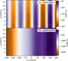 |
Fig. 6. ELBO landscape of the simulated Jones scalars in Fig. 5 during the first and second iterations of Algorithm 1. Top panel: ELBO basin during the first iteration, and lower panel: ELBO basin during the second iteration after one round of parameter estimation. The ground-truth DDTEC is 150 mTECU in this example. |
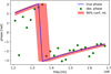 |
Fig. 7. Posterior doubly differential phase solved with variational inference. The shaded region shows the central 90% confidence interval following two passes of Algorithm 1. The resulting variational estimate for DDTEC is 149.1 ± 2.3 mTECU. The ground-truth DDTEC is 150 mTECU. |
To globally optimise ELBO in the presence of many local optima, we use brute force to locate a good starting point, and then use BFGS quasi-Newton optimisation from that point to find the global optimum. Because there are only two variational parameters, the brute-force grid search is very quick.
In this randomly chosen data set 0.1% of the measured DDTEC are found to be outlier solutions, that is, approximately 1.6 × 10³ of 2.6 × 10⁶ optical pathways. Outliers are visually characterised by a posterior uncertainty that is too small to explain its deviation from its neighbouring (in time and direction) DDTEC. Outliers drastically affect the performance of the screen inference step because the uncertainties will be “trusted”.
We detect outliers using a two-part heuristic approach, where we value having more false positives over false negatives. First, we filter for large jumps in DDTEC. We use rolling-statistics sigma-clipping, where we flag DDTEC that deviate by more than two standard deviations from the median in a rolling temporal window of 15 min. Secondly, we filter for large jumps directionally. We fit a smoothed multiquadric radial basis function to the DDTEC over direction and flag outliers where the DDTEC deviates by more than 8 mTECU. Measured DDTEC that are flagged as outliers are given infinite uncertainty.
3.4. Infer DDTEC screen
We denote the DDTEC mean and uncertainties inferred with variational inference in Sect. 3.3 as the measured DDTEC with associated measurement uncertainties. In this section we show how we perform probabilistic inference of a DDTEC screen. In order to distinguish the DDTEC screen from the measured DDTEC, we call them the inferred DDTEC. The process is visualised in the correspondingly labelled box in Fig. 8.
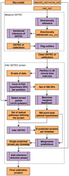 |
Fig. 8. Flow diagram of the measure DDTEC and infer DDTEC screen steps. These steps can be considered the main difference between our method and the method used in the LoTSS-DR1 and DR2 pipelines. |
We define the screen directions by selecting the brightest 250 directions with apparent brightness greater than 0.01 Jy beam−1 and separated by at least 4′. We exclude the original calibrator directions from the set of screen directions, which already have optimal solutions provided in smooth_cal+slow_cal.
We model the measured DDTEC over optical pathways, indexed by (x, k), following the ionospheric model proposed in Albert et al. (2020), which geometrically models the ionosphere as a flat, thick, infinite-in-extent layer with free electron density (FED) realised from a Gaussian process. Whereas in Albert et al. (2020) the modelled quantity was differential total electron content (DTEC), here we model DDTEC, which requires a modification to their model. Generalising the procedure outlined therein, we can arrive at similar expressions as their Eqs. (11) and (14). Because the results can be arrived at by following the same procedure, we do not show the derivation here and simply state the DDTEC prior mean and covariance,
![Mathematical equation: $$ m_{\Delta _0^2\tau }(\boldsymbol{x}, \boldsymbol{k}) = \mathbb{E} [\Delta _0^2\tau (\boldsymbol{x}, \boldsymbol{k})] = 0, $$](/articles/aa/full_html/2020/03/aa37424-19/aa37424-19-eq24.gif) (16)
(16)
![Mathematical equation: $$ \begin{aligned} &K_{\Delta _0^2\tau }((\boldsymbol{x}_i, \boldsymbol{k}), (\boldsymbol{x}_j, \boldsymbol{k}^{\prime} )) = \mathbb{E} [\Delta _0^2\tau (\boldsymbol{x}_i, \boldsymbol{k}) \Delta _0^2\tau (\boldsymbol{x}_j, \boldsymbol{k}^{\prime} )] \\&\qquad \qquad \qquad \qquad \;= I_{ij}^{{\boldsymbol{k}}{\boldsymbol{k}^{\prime} }} -I_{i0}^{{\boldsymbol{k}}{\boldsymbol{k}^{\prime} }} -I_{ij}^{{\boldsymbol{k}}{\boldsymbol{k}}_0} +I_{i0}^{{\boldsymbol{k}}{\boldsymbol{k}}_0}\nonumber \\&\qquad \qquad \qquad \qquad \quad -I_{0j}^{{\boldsymbol{k}}{\boldsymbol{k}^{\prime} }} +I_{00}^{{\boldsymbol{k}}{\boldsymbol{k}^{\prime} }} +I_{0j}^{{\boldsymbol{k}}{\boldsymbol{k}}_0} -I_{00}^{{\boldsymbol{k}}{\boldsymbol{k}}_0}\nonumber \\&\qquad \qquad \qquad \qquad \quad -I_{ij}^{{\boldsymbol{k}}_0{\boldsymbol{k}^{\prime} }} +I_{i0}^{{\boldsymbol{k}}_0{\boldsymbol{k}^{\prime} }} +I_{ij}^{{\boldsymbol{k}}_0{\boldsymbol{k}}_0} -I_{i0}^{{\boldsymbol{k}}_0{\boldsymbol{k}}_0} \end{aligned} $$](/articles/aa/full_html/2020/03/aa37424-19/aa37424-19-eq25.gif) (17)
(17)
 (18)
(18)
where we have used the same notation with Latin subscripts denoting antenna indices. Each term in Eq. (18) is a double integral
 (19)
(19)
of the FED covariance function K, and the integration limits are given by
 (20)
(20)
where a is the height of the centre of the ionosphere layer above the reference antenna, and b is the thickness of the ionosphere layer. The coordinate frame is one where the  is normal to the ionosphere layer, for instance, the east-north-up frame.
The FED kernel, K, that is chosen determines the characteristics of the resulting DDTEC. In Sect. 3.4.1 we discuss our choice of FED kernels. For a comprehensive explanation of the effect of different FED kernels on DTEC and examples of inference with this model, see Albert et al. (2020). Importantly, the only difference between inference of DDTEC and inference of DTEC is in the number of terms in Eq. (18), where there are 16 for DDTEC and only 4 for DTEC.
Using Eqs. (16) and (18) to define the DDTEC prior distribution, we infer the posterior distribution for the DDTEC screen given our measured DDTEC following standard Gaussian process regression formulae (e.g. Rasmussen & Williams 2006). Specifically, given a particular choice for the FED kernel, K, if the set of optical pathways of the measured DDTEC are given by Z and the set of all optical pathways that we wish to infer DDTEC over are given by Z*, then the posterior distribution is (cf. Eq. (19) in Albert et al. 2020)
![Mathematical equation: $$ \begin{aligned} P\left(\Delta _0^2\tau (\mathbf Z ^*) \mid \Delta _0^2\tau (\mathbf Z ), K\right) =\mathcal{N} [\Delta _0^2\tau (\mathbf Z ^*) \mid \mathbf m (\mathbf Z ^*), \mathbf K (\mathbf Z ^*, \mathbf Z ^*)], \end{aligned} $$](/articles/aa/full_html/2020/03/aa37424-19/aa37424-19-eq30.gif) (21)
(21)
where the conditional mean is  , the conditional covariance is
  , and
, and  . The measured DDTEC mean and uncertainties are
  and
and  , respectively. To handle infinite measurement uncertainties, we factor
  into the product of two diagonal matrices, then symmetrically factor the diagonals out of B. The inverted infinities then act to zero-out corresponding columns on right multiplication and rows on left multiplication.
For a given choice of FED kernel, K, the geometric parameters of the ionosphere and FED kernel hyper parameters are determined by maximising the log-marginal likelihood of the measured DDTEC (cf. Eq. (18) in Albert et al. 2020),
![Mathematical equation: $$ \begin{aligned} \log P\left(\Delta _0^2\tau (\mathbf Z ) \mid K\right) = \log \mathcal{N} [\Delta _0^2\tau (\mathbf Z ) \mid 0, \boldsymbol{B}]. \end{aligned} $$](/articles/aa/full_html/2020/03/aa37424-19/aa37424-19-eq37.gif) (22)
(22)
For all our Gaussian process computations we make use of GPFlow (Matthews et al. 2017), which uses auto-differentiation of Tensorflow (Abadi et al. 2015) to expedite complex optimisation procedures on both CPUs and GPUs.
3.4.1. Accounting for a dynamic ionosphere
The ionosphere is very dynamic, with a variety of influencing factors. It can change its overall behaviour in a matter of minutes (e.g. Mevius et al. 2016; Jordan et al. 2017). In our experimentation, we found that choosing the incorrect FED kernel results in very poor quality screens because of a systematic modelling bias.
We delimit two cases of incorrectly specifying the FED kernel. The first is when the true FED covariance is stationary but the spectral properties are incorrectly specified. This can happen, for example, when the character of the ionosphere changes from rough to smooth, or vice versa. The tomographic nature of  then incorrectly infers DDTEC structure that is not there. In the second case, the true FED covariance is non-stationary and a stationary FEED kernel is assumed. This happens, for example, when a travelling ionospheric disturbance (TID) passes over the field of view (van der Tol 2009). In this case, the FED has a locally non-stationary component and the tomographic nature of the DDTEC kernel will incorrectly condition on the TID structures, causing erratic predictive distributions.
Both types of bias can be handled by a dynamic marginalisation over model hypotheses. To do this, we denote each choice of FED kernel as a hypothesis. For each choice of FED kernel, we optimise the FED and ionosphere hyperparameters by maximising the log-marginal likelihood of the measured DDTEC, Eq. (22). We then define the hypothesis-marginalised posterior as
 (23)
(23)
where  . This marginalisation procedure can be viewed as a three-level hierarchical Bayesian model (e.g. Rasmussen & Williams 2006). The hypothesis-marginalised distribution is a mixture of Gaussian distributions, which is a compound model and is no longer Gaussian in general. We approximate the mixture with a single Gaussian by analytically minimising the Kullbeck-Leibler divergence from the mixture to the single Gaussian. For reference, the mean of the single Gaussian approximation is the convex sum of means weighted by the hypothesis weights.
For our FED hypothesis kernels we select the Matérn-p/2 class of kernels for p ∈ {1, 3, 5, ∞} and the rational-quadratic kernel (Rasmussen & Williams 2006). All selected kernels are stationary. While we could incorporate non-stationary FED kernel hypotheses to handle the second type of bias, we do not explore such kernels in this work. See Albert et al. (2020) for examples of the Matérn-p/2 class of FED kernels.
3.4.2. Computational considerations
In order for this approach to be practically feasible, the computation should only require a few hours. The main bottleneck of the computation is computing the 16 double integral terms in Eq. (18) for every pair of optical pathways, and inverting that matrix. A single covariance matrix requires evaluating 16(NresNantNcal)2 double-precision floating point numbers that are stored in a NantNcal × NantNcal matrix. In the case of P126+65, using an abscissa resolution of Nres = 5 as suggested by (Albert et al. 2020), the covariance matrix is approximately 23GB of memory, with approximately 600GB of memory used in intermediate products. The large intermediate products mean that the covariance matrix evaluation is memory bus speed bound. Furthermore, the inversion scales with  . Hyperparameter optimisation requires approximately 200 iterations of hessian-based gradient descent, with each iteration computing the matrix and inverse at least once. Therefore, a lower limit on the number of matrix inversions required for a typical observation with five FED kernel hypotheses is 106. On a single computer with 32 cores and 512 GB of RAM this takes several weeks. Chunking data in time produces modest savings. Using GPUs would make this calculation feasible in just a few hours. However, while GPUs are intrinsically enabled by Tensorflow, we do not currently have access to GPUs with enough memory.
To perform this scalably with enough FED kernel hypotheses to handle the dynamic nature of the ionosphere would require too much computing power for a single measurement set calibration, and unfortunately, a trade-off must be made. Therefore, we first make the approximation that the ionosphere is thin, that is, we let b → 0. When we make this approximation, the double integral terms become
 (24)
(24)
where  . This reduces the memory size of intermediate products by
  approximately from 600 GB to 30 GB, but the size of the matrix is still the same, and the same problem of inverting a large matrix appears many times.
Therefore we introduce a second approximation, that there is no a priori coupling between antennae. When we do this, Eq. (18) becomes
 (25)
(25)
This covariance matrix requires only computing 16(Ncal)2 double-precision floating point numbers and requires inverting an Ncal × Ncal matrix. This is extremely fast, even with CPUs, and the whole P126+65 measurement set can be performed in 50 minutes with five FED kernel hypotheses.
After making these approximations with a stationary FED kernel, it becomes difficult to infer the height of the ionosphere, a. Rather, if the FED kernel is isotropic and parametrised by a length scale, for instance, l, then the marginal likelihood becomes sensitive to the ratio a/l. Therefore it is still possible to learn something of the ionosphere with this approximation.
3.5. Image screen
DDFacet has internal capability for applying solutions during imaging in arbitrary directions (Tasse et al. 2018). DDFacet typically works with its own proprietary solution storage format. To facilitate working with our solutions, we extended DDFacet to work with and recieve the directions layout from H5Parm files whose specifications are defined by LoSoTo (de Gasperin et al. 2019). We convert the smooth_cal+slow_cal solutions to H5Parm format and then convert DDTEC to DTEC by adding back the reference direction phase from smooth_cal.
We use the DDFacet hybrid matching pursuit clean algorithm, with five major cycles, 106 minor cycles, a Briggs robust weight of −0.5 (Briggs 1995), a peak gain factor of 0.001, and clean threshold of 100 μJy beam−1. We initialise the clean mask with the final mask from LoTSS-DR2. All other settings are the same as in the LoTSS-DR2 pipeline and can be found in Shimwell et al. (2019). We also apply the same settings to image the solutions in smooth_cal+slow_cal for comparison purposes later.
4. Results
Figure 9 shows several dimensional slices of the resulting DDTEC screens for LOFAR remote antenna RS508HBA, which is 37 km from the reference antenna. Remote antennae are typically more difficult to calibrate because flux on smaller angular scales (longer baselines) drops off, therefore they are a good choice for showing the performance of the DDTEC measurement and screen inference. The top panel shows the temporal evolution of a single direction. We observe two distinct ionospheric behaviours over the course of the observation. From 0 to 3.5 h the ionosphere is “wild”, with DDTEC variations greater than 150 mTECU, and the variation between time steps are more noise-like. From 3.5 h until the end of the observation, the DDTEC rarely exceeds 10 mTECU, and the variations between time steps are smoother. For comparision, a central antenna within 500 m of the reference antenna typically has DDTEC variations of 10 mTECU. In order to have such a small DDTEC so far from the reference antenna, the FED of the ionosphere should be highly spatially correlated on length scales longer than that baseline. This implies that a structure larger than 50 km, potentially at low altitude, is passing over the array during that time.
 |
Fig. 9. DDTEC screens and temporal profile of LOFAR antenna RS508HBA. The lower four plots show the path-length distortions due to the ionosphere from the perspective of antenna RS508HBA during wild and calm periods. Middle row: inferred DDTEC screen, and the bottom row shows the measured DDTEC screen. The black star indicates the reference direction, hence the DDTEC is always zero in that direction. The top plot shows the DDTEC for a single direction over the course of the observation, and it clearly shows that the temporal behaviour changed around 3.5 h into the observation. |
Because we applied FED model hypothesis marginalisation, we can confirm that the spatial power spectrum indeed changed during these two intervals. During the first half of the observation, coinciding with the “wild” ionosphere, the most highly weighted FED kernel hypothesis was the Matérn-1/2 kernel, followed by the Matérn-3/2 kernel. During the last half of the observation, coinciding with the “calm” ionosphere, the most highly weighted FED kernel hypothesis was the Matérn-3/2 kernel, followed by the Matérn-5/2 kernel.
The change in temporal variation roughness implies that the temporal power spectrum of the FED changed in shape, becoming more centrally concentrated in the last half of the observation. If we apply the frozen-flow assumption, then, over short enough time intervals, the temporal covariance becomes the FED spatial covariance and therefore we expect to see rougher temporal correlations when the spatial correlations become rougher. The frozen-flow assumption is thus supported by the fact that the first and last half of the observations are better described by rough and smooth FED kernels, respectively, matching the temporal behaviour.
The middle and bottom rows of Fig. 9 show the antenna-based DDTEC-screens (showing what the ionosphere looks like from the perspective the antenna) of our inferred DDTEC and measured DDTEC, respectively. The left columns are a slice during the “wild” interval and the right column is a slice during the “calm” interval (points indicated in the temporal profile). We note that during the “calm” time the DDTEC-screens are mostly negative. From Eq. (16) we expect that the DDTEC should be zero on average, which seems at odds with the overall negative DDTEC screen at this time slice. As pointed out in Albert et al. (2020), the mean DTEC, and therefore mean DDTEC, should be zero only in the case of a flat infinite-in-extent ionosphere layer, and then in a model where the ionosphere follows the curvature of the Earth, the mean is not zero. The remote antennae of LOFAR are indeed far enough from the reference antenna to have non-zero mean DDTEC as a result of curvature.
Because we applied the two approximations in Sect. 3.4.2, our model is no longer tomographic, therefore we should not expect super-resolution DDTEC inference as observed in Albert et al. (2020). However, our model still retains the directional coupling of a thin-layer ionosphere model. Therefore, we observe that the reference direction is constrained to have zero DDTEC in the inferred DDTEC screens.
Figure 10 shows, side-by-side, several sources in the LoTSS-DR2 archival image, the smooth_cal+slow_cal image, and the inferred DDTEC screen image. The column numbers correspond to the region indicated in Fig. 2 with red circles, which shows that all selected sources are between calibrators. The LoTSS-DR2 and smooth_cal+slow_cal sources display similar dispersive phase errors, which implies that the isoplanatic assumption was violated in that region of the image at some point during the observation. In the inferred DDTEC screen image the dispersive phase error effects appear less pronounced, indicating that the inferred DDTEC screen provided a better calibration than nearest-neighbour interpolation of the calibrator solutions.
 |
Fig. 10. Comparison of direction dependent effects in regions far from a calibrator. Bottom row: archival LoTSS-DR2 image, the middle row shows the image when smooth_cal+slow_cal is applied, and the top row shows the final image with our inferred DDTEC screen applied. The column numbers correspond to the regions labelled in Fig. 2. |
In order to quantify the improvement to the image quality caused by applying the inferred DDTEC screen, we systematically compare the scale of artefacts in the vicinity around bright sources within the primary beam. We consider an annulus from 12″ to 90″ around all sources brighter than 0.1 Jy beam−1, and calculate the root-mean-squared residuals for the LoTSS-DR2 image, σDR2, and inferred DDTEC screen image, σscreen, within that annulus. Figure 11 shows the histogram of log σscreen/σDR2. In total, 76% of the sources have σscreen < σDR2 with a mean reduction in σscreen of 32% with respect to σDR2.
 |
Fig. 11. Histogram and Gaussian kernel density estimation of the difference in magnitude of root-mean-square residuals in annuli around bright source, screen-corrected, σscreen, over LoTSS-DR2 archival, σDR2. The root-mean-square residuals are calculated within an annulus between 12″ and 90″ centred on sources brighter than 0.1 Jy beam−1. The residuals are primary-beam uncorrected. The black line denotes the mean ratio, and corresponds to σscreen = 0.68σDR2. |
5. Discussion
In P126+65 there is a clear improvement over LoTSS-DR2 resulting from applying our inferred DDTEC screens. Remarkably, we see this improvement using only 35 in-field calibrators compared to the 46 used in LoTSS-DR2. This suggests that the method may have applications to other regimes where calibrators are very sparse, such as in very long baseline interferometry or at ultra-low frequencies.
However, it is unclear whether this observation is typical and if the same method applied to other observations would achieve similar results. One obvious difference between observations is the different layout of sources, and therefore potential calibrators. The distribution of bright sources in P126+65 is relatively uniform over the field of view, which plays to the advantage of our screen inference method. As a result of the approximations in Sect. 3.4.2, the method is no longer tomographic, and sparsity of calibrators could have a significant effect on screen quality. One of the next steps would therefore be to test the performance on a large number of observations. Furthermore, there are potential ways in which to make the tomographic approach computationally efficient and therefore computationally viable, but these require more research.
There is also the question of how robust this method is to various systematics. For example, it is not yet known if unsubtracted compact or diffuse emission could be absorbed during the calibration, as is known to occur if there are too many degrees of freedom during calibration. Another source of uncertainty is the robustness of this method to the behaviour of the ionosphere. In this observation two distinct characteristics of the ionosphere were observed: one “wild” and one “calm”. There are perhaps many more types of ionospheres that could be encountered (e.g. Mevius et al. 2016; Jordan et al. 2017). Because of the FED hypothesis marginalisation, we expect that any new ionosphere should be manageable as long as the calibrators are not too sparse by incorporating the right FED kernel hypotheses.
Furthermore, while the changing ionosphere character may be handled with model weighting, the quality of the inferred DDTEC screens ultimately depends upon the quality of the measured DDTEC. If this method were to be applied to LOFAR-LBA or long-baseline data, the robustness of the DDTEC measurements must be guaranteed. For P126+65, 0.1% of all measured DDTEC were found to be outliers, but this could easily be much larger when there is less flux in the field against which to calibrate, as is the case at lower frequencies and on very long baselines, or when the ionosphere coherence time is shorter than the time interval of calibration (tens of seconds).
The improvements to root-mean-squared residuals near bright sources would be more appreciable with lower thermal noise. An interesting avenue on which to test this method would therefore be multi-epoch observations with tens to hundreds of hours of data. In a deep observation, scattering of emission off of the ionospheric can cause low level structure in the image, mimicking astrophysical sources such as cosmic web accretion shocks that are hidden below the thermal noise. Any wide-field statistical study of faint emission should ensure that such effects are properly calibrated.
6. Conclusion
We have put forward a method for DD calibration and imaging of wide-field low-frequency interferometric data by probabilistically inferring DDTEC for all bright sources (> 0.01 Jy beam−1) in the field of view, using a physics-informed model. In order to do this, we proposed an HMM with variational inference of the forward distribution for measuring DDTEC with uncertainties from Jones scalars solved against isolated calibrators. Isolating the calibrators was found to be important because this gives the Jones scalars well-defined effective directions. We handled the dynamic nature of the ionosphere by marginalising the probabilistic model over a number of FED kernels hypotheses. We only explored stationary hypothesis kernels, therefore this method may not perform well on ionospheres with TIDs.
We tested the method on a randomly selected observation taken from the LoTSS-DR2 archive. The resulting image had fewer direction-dependent effects, and the root-mean-squared residuals around bright sources were reduced by about 32% with respect to the LoTSS-DR2 image. Remarkably, we achieved this improvement using only 35 calibrator directions compared to 46 used in LoTSS-DR2. While these results are promising, the robustness of the method must be verified on more observations.
On 8 December, 2016, the total number of sunspots was 14 ± 1.2 and on 9 December, 2016, it was 20 ± 5.7. The average daily sunspot count in December 2016 was 18.
We use the term “measure DDTEC” purely for distinction between the inferred DDTEC screen discussed in Sect. 3.4. Also, from a philosophical perspective, a measurement is a single realisation of inference.
![Mathematical equation: $ \mathrm{KL}\left[\mathcal{N}[\mu_1, \sigma_1^2] \mid\mid \mathcal{N}[\mu_2, \sigma_2^2]\right] = \frac{1}{2}\left(\frac{\sigma_1^2}{\sigma_2^2} + \frac{(\mu_2-\mu_1)^2}{\sigma_2^2} - 1 + \log\frac{\sigma_2^2}{\sigma_1^2}\right) $](/articles/aa/full_html/2020/03/aa37424-19/aa37424-19-eq46.gif) .
.
If b is conditionally independent of a, then p(a ∣ c) = ∫p(a ∣ b)p(b ∣ c) db = 𝔼b|c[p(a ∣ b)] is the Chapman–Kolmogorov identity.
Acknowledgments
J.G.A. and H.T.I. acknowledge funding by NWO under “Nationale Roadmap Grootschalige Onderzoeksfaciliteiten”, as this research is part of the NL SKA roadmap project. J.G.A. and H.J.A.R. acknowledge support from the ERC Advanced Investigator programme NewClusters 321271. R.J.vW. acknowledges support of the VIDI research programme with project number 639.042.729, which is financed by the Netherlands Organisation for Scientific Research (NWO).
References
- Abadi, M., Agarwal, A., Barham, P., et al. 2015, TensorFlow: Large-Scale Machine Learning on Heterogeneous Systems, Software available from tensorflow.org [Google Scholar]
- Albert, J. G., Oei, M. S. S. L., van Weeren, R. J., Intema, H. T., & Röttgering, H. J. A. 2020, A&A, 633, A77 [NASA ADS] [CrossRef] [EDP Sciences] [Google Scholar]
- Bonnassieux, E., Tasse, C., Smirnov, O., & Zarka, P. 2018, A&A, 615, A66 [NASA ADS] [CrossRef] [EDP Sciences] [Google Scholar]
- Briggs, D. 1995, PhD Thesis, New Mexico Institute of Mining Technology [Google Scholar]
- Cohen, A. S., & Röttgering, H. J. A. 2009, AJ, 138, 439 [NASA ADS] [CrossRef] [Google Scholar]
- Cornwell, T. J., Golap, K., & Bhatnagar, S. 2005, in From Clark Lake to the Long Wavelength Array: Bill Erickson’s Radio Science, eds. N. Kassim, M. Perez, W. Junor, & P. Henning, ASP Conf. Ser., 345, 350 [NASA ADS] [Google Scholar]
- Cotton, W. D., Condon, J. J., Perley, R. A., et al. 2004, in Society of Photo-Optical Instrumentation Engineers (SPIE) Conference Series, eds. J. Oschmann, & M. Jacobus, Proc. SPIE, 5489, 180 [NASA ADS] [CrossRef] [Google Scholar]
- de Gasperin, F., Dijkema, T. J., Drabent, A., et al. 2019, A&A, 622, A5 [NASA ADS] [CrossRef] [EDP Sciences] [Google Scholar]
- Dean, T. A., Singh, S. S., Jasra, A., & Peters, G. W. 2014, Scand. J. Stat., 41, 970 [CrossRef] [Google Scholar]
- Fellgett, P. B., & Linfoot, E. H. 1955, Phil. Trans. R. Soc. London Ser. A, 247, 369 [NASA ADS] [CrossRef] [Google Scholar]
- Hamaker, J. P., Bregman, J. D., & Sault, R. J. 1996, A&AS, 117, 137 [NASA ADS] [CrossRef] [EDP Sciences] [Google Scholar]
- Harrison, I., Camera, S., Zuntz, J., & Brown, M. L. 2016, MNRAS, 463, 3674 [NASA ADS] [CrossRef] [Google Scholar]
- Hensman, J., Fusi, N., & Lawrence, N. D. 2013, ArXiv e-prints [arXiv:1309.6835] [Google Scholar]
- Hewish, A. 1951, Proc. R. Soc. London Ser. A, 209, 81 [NASA ADS] [CrossRef] [Google Scholar]
- Hewish, A. 1952, Proc. R. Soc. London Ser. A, 214, 494 [NASA ADS] [CrossRef] [Google Scholar]
- Intema, H. T., van der Tol, S., Cotton, W. D., et al. 2009, A&A, 501, 1185 [NASA ADS] [CrossRef] [EDP Sciences] [Google Scholar]
- Jones, R. C. 1941, J. Opt. Soc. Am. (1917–1983), 31, 488 [NASA ADS] [CrossRef] [Google Scholar]
- Jordan, C. H., Murray, S., Trott, C. M., et al. 2017, MNRAS, 471, 3974 [NASA ADS] [CrossRef] [Google Scholar]
- Kazemi, S., Yatawatta, S., Zaroubi, S., et al. 2011, MNRAS, 414, 1656 [NASA ADS] [CrossRef] [Google Scholar]
- Kivelson, M. G., & Russell, C. T. 1995, Introduction to Space Physics (Cambridge: Cambridge University Press), 586 [Google Scholar]
- Kolmogorov, A. N. 1960, Foundations of the Theory of Probability, 2nd edn. (London: Chelsea Pub. Co.) [Google Scholar]
- Matthews, A. G. D. G., van der Wilk, M., Nickson, T., et al. 2017, J. Mach. Learn. Res., 18, 1 [Google Scholar]
- Mevius, M., van der Tol, S., Pandey, V. N., et al. 2016, Radio Sci., 51, 927 [NASA ADS] [CrossRef] [Google Scholar]
- Patil, A. H., Yatawatta, S., Koopmans, L. V. E., et al. 2017, ApJ, 838, 65 [NASA ADS] [CrossRef] [Google Scholar]
- Phillips, G. J. 1952, J. Atmos. Terrest. Phys., 2, 141 [NASA ADS] [CrossRef] [Google Scholar]
- Prasad, P., Huizinga, F., Kooistra, E., et al. 2016, J. Astron. Instrum., 5, 1641008 [CrossRef] [Google Scholar]
- Rabiner, L., & Juang, B. 1986, IEEE ASSP Mag., 3, 4 [CrossRef] [Google Scholar]
- Rasmussen, C. E., & Williams, C. K. I. 2006, in Gaussian Processes for Machine Learning (The MIT Press), Adaptive Computation and Machine Learning [Google Scholar]
- Ratcliffe, J. A. 1956, Rep. Progr. Phys., 19, 188 [NASA ADS] [CrossRef] [Google Scholar]
- Rauch, H. E. 1963, IEEE Trans. Autom. Control, AC-8, 371 [CrossRef] [Google Scholar]
- Shimwell, T. W., Röttgering, H. J. A., Best, P. N., et al. 2017, A&A, 598, A104 [NASA ADS] [CrossRef] [EDP Sciences] [Google Scholar]
- Shimwell, T. W., Tasse, C., Hardcastle, M. J., et al. 2019, A&A, 622, A1 [NASA ADS] [CrossRef] [EDP Sciences] [Google Scholar]
- Shumway, R. H., & Stoffer, D. S. 1982, J. Time Ser. Anal., 3, 253 [CrossRef] [Google Scholar]
- Smirnov, O. M., & Tasse, C. 2015, MNRAS, 449, 2668 [NASA ADS] [CrossRef] [Google Scholar]
- Tasse, C. 2014a, ArXiv e-prints [arXiv:1410.8706] [Google Scholar]
- Tasse, C. 2014b, A&A, 566, A127 [NASA ADS] [CrossRef] [EDP Sciences] [Google Scholar]
- Tasse, C., Hugo, B., Mirmont, M., et al. 2018, A&A, 611, A87 [NASA ADS] [CrossRef] [EDP Sciences] [Google Scholar]
- van der Tol, S. 2009, PhD Thesis, TU Delft [Google Scholar]
- van Haarlem, M. P., Wise, M. W., Gunst, A. W., et al. 2013, A&A, 556, A2 [NASA ADS] [CrossRef] [EDP Sciences] [Google Scholar]
- van Weeren, R. J., Williams, W. L., Hardcastle, M. J., et al. 2016, ApJS, 223, 2 [NASA ADS] [CrossRef] [Google Scholar]
- van Weeren, R. J., de Gasperin, F., Akamatsu, H., et al. 2019, Sapce Sci. Rev., 215, 16 [NASA ADS] [CrossRef] [Google Scholar]
- Vernstrom, T., Gaensler, B. M., Brown, S., Lenc, E., & Norris, R. P. 2017, MNRAS, 467, 4914 [NASA ADS] [CrossRef] [Google Scholar]
Appendix A: Factoring commutative DI dependence from the RIME
We consider the effect of directionally referencing spatially referenced commutative Jones scalars. In particular, we study phases of the Jones scalars, and assume amplitudes of one, but the same idea extends to amplitude by considering log-amplitudes that can be treated like a pure-imaginary phase.
Let g(x, k) = eiϕ(x, k) be a Jones scalar, and consider the necessarily non-unique decomposition of phase into DD and DI components,
 (A.1)
(A.1)
This functional form only specifies that the DI term is not dependent on k. The differential phase to which the RIME is sensitive is found by spatially referencing the phase,
 (A.2)
(A.2)
 (A.3)
(A.3)
Directionally referencing the differential phase to direction k0, we have
 (A.4)
(A.4)
 (A.5)
(A.5)
We see that the DI phase has disappeared, and we are left with the doubly differential phase for the DD term. We then assume that there was a remnant DI component in ϕDD(x, k). Then by induction we have that  must be free of DI terms, and
  must be free of all DI components. It follows that directionally referencing phase guarantees that all DI components are removed.
Furthermore, assuming we were to directionally reference a doubly differential phase. We assume that the doubly differential phase is referenced to direction  , with
  . Then we see
 (A.6)
(A.6)
 (A.7)
(A.7)
 (A.8)
(A.8)
That is, directionally referencing a doubly differential phase produces a new doubly differential phase, referenced to the new direction, k0. This trick thus allows us to set a well-defined reference direction to phases that have undergone DI calibration before DD calibration.
Appendix B: Recursive Bayesian estimation
Recursive Bayesian estimation is a method of performing inference on a hidden Markov model (HMM; Rabiner & Juang 1986). Let y be an observable and x be a hidden variable. The HMM assumptions on x and y are, firstly, that the hidden random variable is only conditionally dependent on its previous state, and secondly, the observable is conditionally independent of all other random variables except for the current hidden state. These assumptions are depicted in Fig. B.1, where i is the sequence index. This paradigm is often given a notion of causality or time, but this is not necessary in any way. The sequence index is an abstract notion that simply explains how the set of hidden variables are traversed. For example, we assume that the observations are frames of a movie, and the hidden variable is the plot contained in each movie frame. The HMM assumption is that the movie plot is linear, and the picture encodes what is going on in the movie at a given point in time. With recursive Bayesian estimation the movie can be watched with frames randomly ordered and the complete plot is still rendered completely.
 |
Fig. B.1. Casual graph depicting a hidden Markov model. |
There are two distinct types of information propagation in a hidden Markov model. Information can flow in the direction of the arrows, or against them. This leads to the notion of the forward and backwards equations that describe how belief in hidden variables is propagated forward, and for revising, we believe in previously visited hidden variables.
The joint distribution of the hidden random variables and observables in a chain of length T can be written out as a product of conditional distributions and a marginal using the product rule of probability distributions (Kolmogorov 1960). Because of the HMM assumptions the joint distribution is
 (B.1)
(B.1)
We first consider propagating information forward. This is done in two steps, typically called the predict and update steps. For the predict step, we consider how belief in the absence of new observables is propagated. For this, we apply the Chapman–Kolmogorov identity4 for Markovian processes,
![Mathematical equation: $$ \begin{aligned} p(\boldsymbol{x}_{i+1} \mid \boldsymbol{y}_{0:i}) = \mathbb{E} _{\boldsymbol{x}_{i} \mid \boldsymbol{y}_{0:i}}\left[p(\boldsymbol{x}_{i+1} \mid \boldsymbol{x}_{i}) \right], \end{aligned} $$](/articles/aa/full_html/2020/03/aa37424-19/aa37424-19-eq60.gif) (B.2)
(B.2)
which gives us the probability distribution of the hidden variables at time i + 1 in terms of the so-called state transition distribution p(xi + 1 ∣ xi) and posterior distribution p(xi ∣ y0 : i) at index i. The current prior belief can be understood as the expectation of the state transition distribution over the measure of the current posterior belief.
The update step is simply an application of the Bayes theorem with the prior defined by the predict step,
![Mathematical equation: $$ \begin{aligned} p(\boldsymbol{x}_{i} \mid \boldsymbol{y}_{0:i}) = \frac{{p}(\boldsymbol{y}_{i} \mid \boldsymbol{x}_{i}) \mathbb{E} _{\boldsymbol{x}_{i-1} \mid \boldsymbol{y}_{0:i-1}}\left[p(\boldsymbol{x}_{i} \mid \boldsymbol{x}_{i-1}) \right]}{{p}(\boldsymbol{y}_{i} \mid \boldsymbol{y}_{0:i-1})}, \end{aligned} $$](/articles/aa/full_html/2020/03/aa37424-19/aa37424-19-eq61.gif) (B.3)
(B.3)
where the denominator is the Bayesian evidence of the newly arrived data given all previous data, and it is independent of the hidden variables. Equation (B.3) gives a recurrence relation for propagating our belief forward, therefore this is called the forward equation.
We now assume that we are at index T, and wish to use all acquired information to revise our belief in the previously visited hidden variables at indices i < T. The trick is to realise that p(xi ∣ xi + 1 ∣ y0 : T) = p(xi ∣ xi + 1 ∣ y0 : i) as a result of the Markov properties. In this case, again using the product rule, we find that the joint conditional distribution of a pair of sequential hidden states given the whole sequence of data is
 (B.4)
(B.4)
Marginalising the second hidden parameter, we arrive at the recurrence relation
 (B.5)
(B.5)
This can be solved by starting at T and solving this equation iteratively backwards, therefore Eq. (B.5) is called the backward equation. Most importantly, we note that the backward equation does not require conditioning on data, as was done in the update step.
When the transition and likelihood are assumed to be Gaussian, for example, in a linear dynamical system, the forward and backward equations are equivalent to the well-known Kalman filter equations and Rauch smoother equations (Rauch 1963), respectively.
Appendix C: Jones scalar variational expectation
Let g ∈ ℂNfreq be an observed complex Jones scalar vector, with amplitudes g ∈ ℝNfreq and phases ϕ ∈ ℝNfreq. We assume that the Jones scalars have complex Gaussian noise, described by the observational covariance matrix Σ. Thus, we have that the observational likelihood of the Jones scalars (cf Eq. (9)) is
![Mathematical equation: $$ \begin{aligned} p(\boldsymbol{g} \mid \phi , {g}, \boldsymbol{\Sigma }) = \mathcal{N} _\mathbb{C} [\boldsymbol{g} \mid g e^{\iota \phi }, \boldsymbol{\Sigma }], \end{aligned} $$](/articles/aa/full_html/2020/03/aa37424-19/aa37424-19-eq64.gif) (C.1)
(C.1)
where 𝒩ℂ is the complex Gaussian distribution, which is defined as the Gaussian distribution of the stacked real and imaginary components. We define the residuals δR = Re[g]−g cos ϕ and δI = Im[g]−g sin ϕ, and the stacked residuals δg = (δR, δI)T. Then the log-likelihood becomes
 (C.2)
(C.2)
![Mathematical equation: $$ \begin{aligned} &= -N_{\rm freq} \log 2 \pi - \frac{1}{2}\log |\boldsymbol{\Sigma }| - \frac{1}{2} \mathrm{Tr} [\boldsymbol{\Sigma }^{-1} \delta \boldsymbol{g} \delta \boldsymbol{g}^T] \end{aligned} $$](/articles/aa/full_html/2020/03/aa37424-19/aa37424-19-eq66.gif) (C.3)
(C.3)
![Mathematical equation: $$ \begin{aligned} \\&= -N_{\rm freq} \log 2 \pi - \frac{1}{2} \log |\boldsymbol{\Sigma }| - \frac{1}{2} \mathrm{vec} [\boldsymbol{\Sigma }^{-1}]^{T} \mathrm{vec} [\delta \boldsymbol{g} \delta \boldsymbol{g}^T] \end{aligned} $$](/articles/aa/full_html/2020/03/aa37424-19/aa37424-19-eq67.gif) (C.4)
(C.4)
where we used the fact that the trace of a scalar is a scalar, and that Tr[ATB] = Tr[BAT] = vec[A]Tvec[B].
Now we assume that the phases are linearly modelled according to
 (C.5)
(C.5)
where fi(ν) is the ith basis function of a set of M linearly independent functions depending on frequency ν, and ai is the ith parameter in the linear model. We furthermore assume that each parameter ai is a Gaussian random variable,
![Mathematical equation: $$ \begin{aligned} a_i \sim \mathcal{N} [m_i, l_i^2], \end{aligned} $$](/articles/aa/full_html/2020/03/aa37424-19/aa37424-19-eq69.gif) (C.6)
(C.6)
and that all parameters are independent, that is, p(ai, aj) = p(ai)p(aj). Because all parameters are independent and the basis functions are linearly independent, the phase is the unique Gaussian random variable with distribution,
![Mathematical equation: $$ \begin{aligned} p(\phi (\nu )) = \mathcal{N} \left[\sum _i^M f_i(\nu ) m_i, \sum _i^M f^2_i(\nu ) l_i^2\right]. \end{aligned} $$](/articles/aa/full_html/2020/03/aa37424-19/aa37424-19-eq70.gif) (C.7)
(C.7)
The variational expectation of the Jones scalars with respect to the phase is thus defined as
![Mathematical equation: $$ \begin{aligned} \mathbb{E} _{{p}(\phi )}\left[\log p(\boldsymbol{g} \mid \phi , {g}, \boldsymbol{\Sigma }) \right]&= -N_{\rm freq} \log 2 \pi -\frac{1}{2} \log |\boldsymbol{\Sigma }| \nonumber \\ &\quad - \frac{1}{2} \mathrm{vec} [\boldsymbol{\Sigma }^{-1}]^T \mathrm{vec} \left[\mathbb{E} _{{p}(\phi )}[\delta \boldsymbol{g} \delta \boldsymbol{g}^T]\right], \end{aligned} $$](/articles/aa/full_html/2020/03/aa37424-19/aa37424-19-eq71.gif) (C.8)
(C.8)
where we used that expectation and the vectorisation operator commute. Now we need to evaluate the expectation, 𝔼p(ϕ)[δgδgT]. In order to do this, we realise that there are three explicit integrations that must be done corresponding to unique sub-blocks of δgδgT consisting of the real–real, real–imaginary, and imaginary–imaginary outer products of residual vectors,
![Mathematical equation: $$ \begin{aligned} \mathbb{E} _{{p}(\phi )}\left[\delta R \delta R^T\right]&= \int \delta R \delta R^T\, \mathrm{d} p(\phi ) \end{aligned} $$](/articles/aa/full_html/2020/03/aa37424-19/aa37424-19-eq72.gif) (C.9)
(C.9)
 (C.10)
![Mathematical equation: $$ \mathbb{E} _{{p}(\phi )}\left[ \delta R \delta I^T\right]= \int \delta R \delta I^T\, \mathrm{d} p(\phi ) $$](/articles/aa/full_html/2020/03/aa37424-19/aa37424-19-eq74.gif) (C.11)
(C.11)
 (C.12)
![Mathematical equation: $$ \begin{aligned} \mathbb{E} _{{p}(\phi )}\left[\delta I \delta I^T\right]&= \int \delta I\delta I^T\, \mathrm{d} p(\phi ) \end{aligned} $$](/articles/aa/full_html/2020/03/aa37424-19/aa37424-19-eq76.gif) (C.13)
(C.13)
 (C.14)
All three of the above integrals involve Gaussian expectations of trigonometric functions. For example the (i, j)th element of the integral Irr is,
![Mathematical equation: $$ \begin{aligned} (I_{\rm rr})_{(i,j)} = \int (\mathrm{Re} [\boldsymbol{g}]_i - {g}_i \cos \phi (\nu _i)) (\mathrm{Re} [\boldsymbol{g}]_j - {g}_j \cos \phi (\nu _j))\, \mathrm{d} p(\phi (\nu _i), \phi (\nu _j)). \end{aligned} $$](/articles/aa/full_html/2020/03/aa37424-19/aa37424-19-eq78.gif) (C.15)
(C.15)
To evaluate this integral, we use Euler’s formulae, for example, for cosine, 2 cos ϕ = eiϕ + e−iϕ. This allows us to reduce all combinations of trigonometric functions to complex exponentials. We then use the characteristic function of the Gaussian distribution, which gives the relation, ![Mathematical equation: $ \mathbb{E}_{X \sim \mathcal{N}[m, l^2]}[\mathrm{e}^{i X}] = \mathrm{e}^{i m - \frac{l^2}{2}} $](/articles/aa/full_html/2020/03/aa37424-19/aa37424-19-eq79.gif) . Applying the above, after significant elementary algebraic work, we evaluate all integral matrix elements,
. Applying the above, after significant elementary algebraic work, we evaluate all integral matrix elements,
![Mathematical equation: $$ \begin{aligned} (I_{rr})_{(i,j)}&= \mathrm{Re} [\boldsymbol{g}]_i \mathrm{Re} [\boldsymbol{g}]_j - e^{-\theta _i} g_i\mathrm{Re} [\boldsymbol{g}]_j \cos \phi _i - e^{-\theta _j} g_j \mathrm{Re} [\boldsymbol{g}]_i \cos \phi _j\nonumber \\&\quad + \frac{1}{2}e^{\theta _{ij}^-} g_i g_j\cos \phi _{ij}^- + \frac{1}{2}e^{-\theta _{ij}^+} g_i g_j\cos \phi _{ij}^+ \end{aligned} $$](/articles/aa/full_html/2020/03/aa37424-19/aa37424-19-eq80.gif) (C.16)
(C.16)
![Mathematical equation: $$ \begin{aligned} (I_{ri})_{(i,j)}&= \mathrm{Re} [\boldsymbol{g}]_i \mathrm{Im} [\boldsymbol{g}]_j - e^{-\theta _i} g_i \mathrm{Im} [\boldsymbol{g}]_j \cos \phi _i - e^{-\theta _j} g_j \mathrm{Re} [\boldsymbol{g}]_i \sin \phi _j\nonumber \\&\quad - \frac{1}{2}e^{\theta _{ij}^-} g_i g_j\sin \phi _{ij}^- + \frac{1}{2}e^{-\theta _{ij}^+} g_i g_j\sin \phi _{ij}^+ \end{aligned} $$](/articles/aa/full_html/2020/03/aa37424-19/aa37424-19-eq81.gif) (C.17)
(C.17)
![Mathematical equation: $$ \begin{aligned} (I_{ii})_{(i,j)}&= \mathrm{Im} [\boldsymbol{g}]_i \mathrm{Im} [\boldsymbol{g}]_j - e^{-\theta _i} g_i \mathrm{Im} [\boldsymbol{g}]_j \sin \phi _i - e^{-\theta _j} g_j\mathrm{Im} [\boldsymbol{g}]_i \sin \phi _j\nonumber \\&\quad + \frac{1}{2}e^{\theta _{ij}^-} g_i g_j\cos \phi _{ij}^- - \frac{1}{2}e^{-\theta _{ij}^+} g_i g_j\cos \phi _{ij}^+ \end{aligned} $$](/articles/aa/full_html/2020/03/aa37424-19/aa37424-19-eq82.gif) (C.18)
(C.18)
where,
 (C.19)
 (C.20)
 (C.21)
 (C.22)
This completes the evaluation of Eq. (C.8) for an arbitrary linear phase model. For example, in a phase model consisting only of DDTEC, we have M = 1,  and
and  . It is simple to calculate the variational expectation of other linear phase models including terms such as clock-like terms, constant-in-frequency terms, and higher order ionospheric terms.
All Figures
|
Fig. 1. Flow diagram overview of our DD calibration and imaging program. |
| In the text | |
|
Fig. 2. Layout of our selected calibrators (black stars) compared to the LoTSS-DR2 archival calibrator layout (cyan circles). The calibrators define a facet tessellation of the field of view. The red circles indicate the regions of the cutouts in Fig. 10. |
| In the text | |
|
Fig. 3. Example of an average effective direction in a facet. The red circles indicate calibrators. The central calibrator has a peak flux of 0.91 Jy beam−1, while the next brightest non-calibrator source, approximately 16′ to the left, is 0.12 Jy beam−1. Within the facet of the calibrator, the Jones matrices are mostly optimised in a direction of the calibrator, but this effective direction changes over time, baseline, and frequency. |
| In the text | |
|
Fig. 4. Flow chart of the subtract and solve and smooth and slow-resolve steps. Together, they represent a DD calibration program similar to the LoTSS-DR1 and DR2 pipelines. |
| In the text | |
|
Fig. 5. Simulated real and imaginary components of noise-dominated Jones scalars and observational uncertainties. The simulated ground truth DDTEC is 150 mTECU and the observational uncertainties are frequency dependent and correlated, corresponding to a remote station for a calibrator at the cutoff peak flux limit of 0.3 Jy beam−1. |
| In the text | |
|
Fig. 6. ELBO landscape of the simulated Jones scalars in Fig. 5 during the first and second iterations of Algorithm 1. Top panel: ELBO basin during the first iteration, and lower panel: ELBO basin during the second iteration after one round of parameter estimation. The ground-truth DDTEC is 150 mTECU in this example. |
| In the text | |
|
Fig. 7. Posterior doubly differential phase solved with variational inference. The shaded region shows the central 90% confidence interval following two passes of Algorithm 1. The resulting variational estimate for DDTEC is 149.1 ± 2.3 mTECU. The ground-truth DDTEC is 150 mTECU. |
| In the text | |
|
Fig. 8. Flow diagram of the measure DDTEC and infer DDTEC screen steps. These steps can be considered the main difference between our method and the method used in the LoTSS-DR1 and DR2 pipelines. |
| In the text | |
|
Fig. 9. DDTEC screens and temporal profile of LOFAR antenna RS508HBA. The lower four plots show the path-length distortions due to the ionosphere from the perspective of antenna RS508HBA during wild and calm periods. Middle row: inferred DDTEC screen, and the bottom row shows the measured DDTEC screen. The black star indicates the reference direction, hence the DDTEC is always zero in that direction. The top plot shows the DDTEC for a single direction over the course of the observation, and it clearly shows that the temporal behaviour changed around 3.5 h into the observation. |
| In the text | |
|
Fig. 10. Comparison of direction dependent effects in regions far from a calibrator. Bottom row: archival LoTSS-DR2 image, the middle row shows the image when smooth_cal+slow_cal is applied, and the top row shows the final image with our inferred DDTEC screen applied. The column numbers correspond to the regions labelled in Fig. 2. |
| In the text | |
|
Fig. 11. Histogram and Gaussian kernel density estimation of the difference in magnitude of root-mean-square residuals in annuli around bright source, screen-corrected, σscreen, over LoTSS-DR2 archival, σDR2. The root-mean-square residuals are calculated within an annulus between 12″ and 90″ centred on sources brighter than 0.1 Jy beam−1. The residuals are primary-beam uncorrected. The black line denotes the mean ratio, and corresponds to σscreen = 0.68σDR2. |
| In the text | |
|
Fig. B.1. Casual graph depicting a hidden Markov model. |
| In the text | |
Current usage metrics show cumulative count of Article Views (full-text article views including HTML views, PDF and ePub downloads, according to the available data) and Abstracts Views on Vision4Press platform.
Data correspond to usage on the plateform after 2015. The current usage metrics is available 48-96 hours after online publication and is updated daily on week days.
Initial download of the metrics may take a while.