| Issue |
A&A
Volume 635, March 2020
|
|
|---|---|---|
| Article Number | A173 | |
| Number of page(s) | 14 | |
| Section | Stellar atmospheres | |
| DOI | https://doi.org/10.1051/0004-6361/201937150 | |
| Published online | 02 April 2020 | |
Stellar wind models of central stars of planetary nebulae
1
Ústav teoretické fyziky a astrofyziky, Masarykova univerzita,
Kotlářská 2,
611,
37 Brno,
Czech Republic
e-mail: This email address is being protected from spambots. You need JavaScript enabled to view it.
2
Astronomický ústav, Akademie věd České republiky,
Fričova 298,
251 65
Ondřejov,
Czech Republic
Received:
20
November
2019
Accepted:
26
February
2020
Abstract
Context. Fast line-driven stellar winds play an important role in the evolution of planetary nebulae, even though they are relatively weak.
Aims. We provide global (unified) hot star wind models of central stars of planetary nebulae. The models predict wind structure including the mass-loss rates, terminal velocities, and emergent fluxes from basic stellar parameters.
Methods. We applied our wind code for parameters corresponding to evolutionary stages between the asymptotic giant branch and white dwarf phases for a star with a final mass of 0.569 M⊙. We study the influence of metallicity and wind inhomogeneities (clumping) on the wind properties.
Results. Line-driven winds appear very early after the star leaves the asymptotic giant branch (at the latest for Teff ≈ 10 kK) and fade away at the white dwarf cooling track (below Teff = 105 kK). Their mass-loss rate mostly scales with the stellar luminosity and, consequently, the mass-loss rate only varies slightly during the transition from the red to the blue part of the Hertzsprung–Russell diagram. There are the following two exceptions to the monotonic behavior: a bistability jump at around 20 kK, where the mass-loss rate decreases by a factor of a few (during evolution) due to a change in iron ionization, and an additional maximum at about Teff = 40−50 kK. On the other hand, the terminal velocity increases from about a few hundreds of km s−1 to a few thousands of km s−1 during the transition as a result of stellar radius decrease. The wind terminal velocity also significantly increases at the bistability jump. Derived wind parameters reasonably agree with observations. The effect of clumping is stronger at the hot side of the bistability jump than at the cool side.
Conclusions. Derived fits to wind parameters can be used in evolutionary models and in studies of planetary nebula formation. A predicted bistability jump in mass-loss rates can cause the appearance of an additional shell of planetary nebula.
Key words: stars: winds, outflows / stars: mass-loss / stars: early-type / stars: AGB and post-AGB / white dwarfs / planetary nebulae: general
© ESO 2020
1 Introduction
The transition between the asymptotic giant branch (AGB) and white dwarf (WD) phases belongs to one of the most prominent phases of stellar evolution. After leaving the AGB phase, the stars for which the expansion time of the AGB envelope is comparable to the transition time-scale create planetary nebulae (Kwok 2008). During this phase, the hot central star of planetary nebula (CSPN) ionizes the material left over from previous evolutionary phases and fast wind of the central star collides with slow material lost during previous evolution (Schönberner et al. 2005). This creates a magnificent nebula that is visible from extragalactic distances (e.g., Herrmann et al. 2008; Richer & McCall 2008).
Although evolutionary tracks after leaving the AGB phase are rather simple (Vassiliadis & Wood 1994; Bloecker 1995), their detailed properties are sensitive to processes occurring during previous evolutionary phases (Miller Bertolami 2016). The detailed treatment of opacities, nuclear reaction rates, and AGB mass-loss affects the predictions of evolutionary models. Yet there is another process that appears after leaving the AGB branch that may affect the evolutionary timescales and appearance of CSPNe: a stellar wind in post-AGB and CSPN phases.
Stellar winds of CSPNe are driven in a similar way as winds of their more massive counterparts, that is, by light absorption and scattering in the lines of heavier elements, including carbon, nitrogen, oxygen, and iron (Pauldrach et al. 1988). The mass-loss rate of hot star winds mainly depends on the stellar luminosity (Castor et al. 1975) and since the winds are primarily driven by heavier elements, also on metallicity (Vink et al. 2001; Krtička 2014). On the other hand, wind terminal velocity, which is the wind velocity at large distances from the star, mainly depends on the surface escape speed (Castor et al. 1975; Lamers et al. 1995).
Stellar winds of CSPN are accessible for observation at intermediate evolutionary stages between AGB and WD. Observational probes of CSPN winds include ultraviolet (UV) P Cygni line profiles and Hα emission (Kudritzki et al. 2006; Herald & Bianchi 2011) and possibly also X-rays (Chu et al. 2001; Guerrero 2006). The observational studies enabled us to derive the wind parameters, that is, the wind mass-loss rate and the terminal velocity.
On the other hand, the stellar winds in the phase immediately following the AGB phase (the post-AGB phase) and at the top of the WD cooling track are difficult to probe observationally due to a fast speed of evolution and weak winds, respectively. However, the winds can be very important even in these elusive stages. Strong winds in a post-AGBphase may affect the duration of this phase (Miller Bertolami 2016) and winds in hot WDs may prevent gravitational settling (Unglaub & Bues 2000), thus explaining near-solar abundances in these stars (Werner et al. 2017, 2018).
To better understand the final evolutionary stages of solar-mass stars, we provide theoretical models of their stellar winds. We used our own wind code to predict wind properties of the stars that just left the AGB phase, CSPNe, and the stars that started their final descend along the WD cooling sequence.
2 Description of the CMF wind models
The wind models of CSPNe were calculated using the global (unified) code METUJE (Krtička & Kubát 2010, 2017). The global models provide self-consistent structure of the stellar photosphere and radiatively-driven wind and, therefore, avoid artificial splitting of these regions. The code solves the radiative transfer equation, the kinetic (statistical) equilibrium equations, and hydrodynamic equations from a nearly hydrostatic photosphere to supersonically expanding wind. The code assumes stationary (time-independent) and spherically symmetric wind.
The radiative transfer equation was solved in the comoving frame (CMF) after Mihalas et al. (1975). In the CMF radiative transfer equation, we account for line and continuum transitions of elements given in Table 1, which are relevant in atmospheres of CSPNe. The inner boundary condition for the radiative transfer equation was derived from the diffusion approximation.
The ionization and excitation state of considered elements (listed in Table 1) was calculated from the kinetic equilibrium equations, which are also called the statistical equilibrium or NLTE equations. These equations account for the radiative and collisional excitation, deexcitation, ionization (including Auger ionization), and recombination. Part of the models of ions was adopted from the TLUSTY model stellar atmosphere input data (Lanz & Hubeny 2003, 2007, denoted as 1 in Table 1). The remaining ionic models given in Table 1 were prepared using the same strategy as in TLUSTY, that is, the data are based on the Opacity and Iron Projectcalculations (Seaton et al. 1992; Hummer et al. 1993) or they were downloaded from the NORAD webpage1 and corrected with the level energies and oscillator strengths available in the NIST database (Kramida et al. 2015). The models of phosphorus ions were prepared using the data described by Pauldrach et al. (2001). The models of ions are based on a superlevel concept as in Lanz & Hubeny (2003, 2007), that is, the low-lying levels are included explicitly, while the higher levels are merged into superlevels. The bound-free radiative rates in kinetic equilibrium equations are consistently calculated from the CMF mean intensity. However, for the bound–bound rates, we used the Sobolev approximation, which can be easily linearized for iterations.
We applied three different methods to solve the energy equation. In the photosphere, we used differential and integral forms of the transfer equation (Kubát 1996), while we applied the electron thermal balance method (Kubát et al. 1999) in the wind.Individual terms in these equations are taken from the CMF radiative field. The energy equations together with the remaining hydrodynamical equations, that is, the continuity equation and the equation of motion, were solved iteratively to obtain the wind density, velocity, and temperature structure. These iterations were performed using the Newton–Raphson method. The models include the radiative force due to line and continuum transitions calculated from the CMF radiative field. However, to avoid possible negative velocity gradients in the photosphere, we limited the continuum radiative force there to a multiple (typically 2) of the radiative force due to the light scattering on free electrons. The line data for the calculation of the line force (see Table 1) were taken from the VALD database (Piskunov et al. 1995, Kupka et al. 1999) with some updates using the NIST (Kramida et al. 2015) and Kurucz (1992) data. For Fe VIII – Fe X, we used line data from the Kurucz website2.
Our model predicts flow structure as a function of the base velocity, which combined with the density gives the mass-loss rate. The code searches for such a value of the mass-loss rate that allows the solution to smoothly pass through the wind critical point, where the wind velocity is equal to the speed of radiative-acoustic waves (Abbott 1980; Thomas & Feldmeier 2016). We calculated a series of wind models with variable base velocity and searched for the base velocity, which provides a smooth transonic solution with a maximum mass-loss rate using the “shooting method” (Krtička & Kubát 2017).
We used the TLUSTY plane-parallel static model stellar atmospheres (Lanz & Hubeny 2003, 2007) to derive the initial estimate of photospheric structure and to compute the emergent fluxes for comparison purposes. The TLUSTY models werecalculated for the same effective temperature, surface gravity, and chemical composition as the wind models.
The wind models were calculated with stellar parameters (given in Table 2) taken from the post-AGB evolutionary tracks of Vassiliadis & Wood (1994, see also Fig. 1). We selected the track with an initial (main-sequence) mass of 1 M⊙, a helium abundance of 0.25, and a metallicity of 0.016, which yields a CSPN mass of M = 0.569 M⊙. This corresponds to a typical mass of CSPN and white dwarfs, which is about 0.55−0.65 M⊙ (e.g., Koester 1987; Stasińska et al. 1997; Kudritzki et al. 2006; Voss et al. 2007; Falcon et al. 2010). Although some deviations of the chemical compositions of CSPN atmospheres from the solar chemical composition can be expected as a result of stellar evolution, most CSPNe and their nebulae have near-solar chemical composition (e.g., Stasińska et al. 1998; Wang & Liu 2007; Milingo et al. 2010). Therefore, we assumed solar abundances Z⊙ according to Asplund et al. (2009).
To get a better convergence, our code assumes an inner boundary radius that is fixed deep in the photosphere. As a result of this, for a given stellar luminosity, the conventionally defined stellar radius is slightly higher and the effective temperature is slightly lower than what is assumed here. This is not a problem for the stars with a higher gravity (with thin atmospheres), but this may have a larger impact on atmospheric models of the stars with lower effective temperatures, which have more extended atmospheres.
Our code finds the wind critical point, which appears slightly above the photosphere. There the mass-loss rate of our models is determined. In some cases, when the initial range of radii was too narrow, the code was unable to find the critical point. A simple solution would be to extend the subcritical model to include the region of the critical point. In some cases, this simple approach failed during subsequent iterations, even if another calculation with a different initial estimate of the solution was able to find a physical solution. This is most likely caused by a complex wind structure that is close to the photosphere, where the temperature bump exists, which significantly influences the density distribution of the subsonic part of the wind. A similar problem can also appear in the codes that use direct integration of hydrodynamical equations.
For some stellar parameters (denoted using an asterisk in Table 2), we were unable to get converged global models. For these models, we calculated core-halo models with TLUSTY model atmosphere emergent flux as a boundary condition (Krtička & Kubát 2010). This may lead to a slight overestimation of the mass-loss rate (Krtička & Kubát 2017) for these particular models.
Atoms and ions included in the NLTE and line force calculations.
3 Calculated wind models
Parameters of calculated wind models (mass-loss rates Ṁ and terminal velocities v∞) are given in Table 2. The wind mass-loss rate mostly depends on the stellar luminosity (e.g., Castor et al. 1975; Vink et al. 2001; Sander et al. 2017; Krtička & Kubát 2017); consequently, the mass-loss rate is nearly constant (on the order of 10−9 M⊙ yr−1) during the evolution of a star from the AGB to the top of the white dwarf cooling track. The mass-loss rate increases with temperatureby more than an order of magnitude for the coolest stars at the beginning of the adopted evolutionary tracks. This is caused by the increase in the UV flux for frequencies that are higher than that of the Lyman jump where most of the strong resonance lines, which drive the wind, appear. When the star settles on the white dwarf cooling track, its luminosity starts to decrease leading to the decrease in the mass-loss rate. We have not found any winds for stars at the white dwarf cooling track after reaching effective temperatures lower than about 100 kK (Fig. 1).
Figure 2 shows the relative contribution of individual elements to the radiative force at the critical point. From Fig. 2, it follows that winds of CSPN are mostly accelerated by C, O, Ne, Mg, and Fe. The contribution of individual elements to the radiative force strongly varies with effective temperature due to changes in the ionization structure. This is demonstrated in the plot of the mean ionization degree that mostly contributes to the radiative force (Fig. 2). The degree changes from III for the coolest stars to VII for the hottest stars. The wind mass-loss rate is relatively high around Teff ≈ 20 kK; consequently, iron lines are optically thick and dominate the radiative driving (Vink et al. 2001). With an increasing temperature, iron ionizes from Fe III to Fe IV, which accelerates the wind less efficiently. Consequently, lighter elements, such as carbon, oxygen, and silicon, take over the wind acceleration. However, for even higher temperatures, these elements appear in closed shell configurations as a He-like ion (carbon) and a Ne-like ion (silicon). These ions have resonance lines around 10 Å, where the stellar flux is low, and as a result they do not significantly accelerate the wind. On the other hand, neon and magnesium, with abundances that are higher than silicon, appear in open shell configurations with a larger number of lines that are capable of driving the wind at higher temperatures.
The wind mass-loss rate mostly depends on the stellar luminosity, which is constant during the post-AGB evolution. As a result, Table 2 mostly shows just mild variations of the mass-loss rate with temperature, connected with changes of contribution of individual ions to the radiative force during the evolution (Fig. 2). Models around Teff = 20 kK most significantly deviate from this behavior. The mass-loss rate from the model T18 to the model T29 decreases by a factor of about 8. This is caused by the decrease in the contribution of iron to the radiative driving (see Fig. 2). Iron around Teff = 20 kK ionizes from Fe III to Fe IV, which accelerates the wind less efficiently. This is accompanied by the increase in the terminal velocity. The behavior of the mass-loss rate and of the terminal velocity corresponds to the bistability jump around Teff ≈ 21 kK, which is found in wind models of B supergiants (Pauldrach & Puls 1990; Vink et al. 1999; Vink 2018). However, the observational behavior of the mass-loss rates of B supergiants around the jump does not seem to follow the theoretical expectations (Crowther et al. 2006; Markova & Puls 2008; Haucke et al. 2018). The reason for different behavior of observationally determined mass-loss rates is unclear and is likely caused by inadequate wind models used to determine the mass-loss rates either from observations or from theory.
There is another broad and weak maximum of the mass-loss rates around Teff = 45 kK, which was also found in the models of Pauldrach et al. (2004). The maximum is caused by a higher radiative flux in the far-UV domain (cf. the flux distributions of T35 and T44 models in Fig. 3), which leads to an increase in the radiative force due to Fe V (Fig. 2).
Another case that deviates from strict Ṁ ~ L dependence is the T116 model. Although the corresponding star has a slightly lower luminosity than that of the T111 model, the mass-loss rate of T116 is higher than the mass-loss rate of the T111 model (see Table 2). This is caused by the change in the ionization of magnesium that most significantly contributes to the radiative force at these temperatures (see Fig. 2). In most cases, higher ionization leads to a weaker radiative force, but Mg VII has more resonance lines that are close to the flux maximum than Mg VI; consequently, as a result of higher ionization, the radiative force and the mass-loss rate increase in this case. The increase in the mass-loss rate is accompanied by the decrease in the terminal velocity (Table 2). This behavior of the mass-loss rate and the terminal velocity resembles the bistability jump around Teff ≈ 20 kK, which is dueto the change in iron ionization (Pauldrach & Puls 1990; Vink 2018).
The wind mass-loss rate of the calculated models on the leftward (heating) part of the evolutionary track can be fit as a function of the effective temperature with a sum of four Gaussians
![Mathematical equation: \begin{equation*}\dot M(T_{\textrm{eff}},L,Z)=\left({\frac{L}{10^3\,L_{\odot}}}\right)^{\alpha} \left({\frac{Z}{Z_{\odot}}}\right)^{\zeta} \sum_{i=1}^4 m_i \exp\left[{-\left({\frac{T_{\textrm{eff}}-T_i}{\Delta T_i}}\right)^2}\right], \end{equation*}](/articles/aa/full_html/2020/03/aa37150-19/aa37150-19-eq1.png) (1)
(1)
where mi, Ti, and ΔTi are parameters of the fit given in Table 3. Equation (1) fits the numerical results with an average precision of about 10%. To account for the dependence of the wind mass-loss rate on the stellar luminosity, we introduced the additional parameter α in Eq. (1), which was kept fixed during fitting. We adopted its value from O star wind models (Krtička & Kubát 2017, Eq. (11)). The metallicity dependence parameter ζ was derived by fitting results of nonsolar metallicity models (see Sect. 5), assuming a solar mass fraction of heavy elements Z⊙ after Asplund et al. (2009). Equation (1) can only be used for the stars within the studied temperature range, that is, for Teff = 10−117 kK.
Wind terminal velocity is proportional to the surface escape speed (e.g., Castor et al. 1975; Lamers et al. 1995; Crowther et al. 2006). The stellar luminosity is constant after leaving the AGB phase, but the effective temperature increases and, therefore, the stellar radius decreases. As a result, the surface escape speed rises and, in addition, the wind terminal velocity increases from 100 to about 4000 km s−1. The wind driving becomes less efficient when the star approaches the white dwarf cooling track; therefore, with a decreasing mass-loss rate, the wind terminal velocity also decreases.
In Fig. 3 we compare emergent fluxes from our global models with fluxes derived from plane-parallel TLUSTY photospheremodels. There is relatively good agreement between these fluxes for frequencies below the Lyman jump. However, for Teff ≲ 40 kK, the global models predict significantly lower fluxes in the region of Lyman continuum due to the blocking of radiation by the stellar wind and due to deviations from spherical symmetry (Kunasz et al. 1975; Kubát 1997). These trends are also apparent in Table 4 where we give the number of ionizing photons per unit of surface area
 (2)
(2)
where Hν is the Eddington flux and the ionization frequency ν0 corresponds to ionization frequencies of H I, He I, and He II. From the table, it follows that the number of H I ionizing photons can be derived from plane–parallel photospheric models for Teff ≳ 40 kK and that the plane-parallel models predict a reliable number of He I ionizing photons for Teff ≳ 50 kK. On the other hand, wind absorption above the He II ionization jump is so strong that the plane–parallel models never predict the correct number of He II ionizing photons for any star with wind. However, even global models are not able to predict He II ionizing flux reliably because there are even significant differences in predicting the He II ionizing flux between individual global models (Puls et al. 2005).
Our derived number of H I and He I ionizing photons for the models T35 and T44 agree typically within 0.1–0.2 dex with the results for dwarfs and supergiants that are published elsewhere (Mokiem et al. 2004; Puls et al. 2005; Martins et al. 2005a). However, the differences in He II ionizing photons (Pauldrach et al. 2001) are more significant and reflect involved model assumptions.
In Table 5 we list the most prominent metallic wind lines in predicted spectra that can be used to search for wind signatures in CSPN spectra. As the wind becomes more ionized for stars with higher effective temperatures, higher ions become visible in the spectra and the most prominent wind features shift toward lower wavelengths.
Adopted stellar parameters (after Vassiliadis & Wood 1994) of the model grid and predicted wind parameters for M = 0.569 M⊙ and Z = Z⊙.
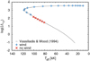 |
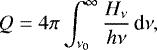
Fig. 1 Adopted evolutionary track of the star with CSPN mass M = 0.569 M⊙ in HR diagram. Blue plus symbols and red crosses denote the locations of studied models from Table 2 with and without wind. |
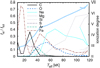 |
Fig. 2 Relative contribution of individual elements to the radiative force at the critical point as a function of the effective temperature. Thick blue line denotes the mean ionization degree that contributes to the radiative force, ∑fizi∕∑fi), where zi is the charge of ion i and fi is its contribution to the radiative force. |
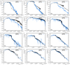 |
Fig. 3 Comparison of the emergent flux from TLUSTY (black line) and METUJE (blue line) models smoothed by a Gaussian filter. The graphs are plotted for individual models from Table 2 (denoted in the plots). |
Calculated number of ionizing photons per unit of surface area  .
.
Wavelengths (in Å) of the most prominent metallic wind lines in individual models.
4 Comparison with observations
Before Gaia Data Release 2 (Gaia Collaboration 2018, hereafter DR2), the observational estimates of CSPN mass-loss rates were problematic due to poorly known distances. To overcome this, Pauldrach et al. (2004) used hydrodynamical wind models to fit the wind line profiles and to estimate the stellar radius (or luminosity) and mass. On the other hand, Herald & Bianchi (2011) provide two sets of stellar and wind parameters; one was derived assuming the most likely stellar mass of CSPNe is about 0.6 M⊙ (adopted here) and second one was derived when using various estimates for distances.
In Fig. 4 we compare our predicted wind mass-loss rates with observational and theoretical results for hydrogen-rich CSPNe as a function of effective temperature. For a reliable determination of mass-loss rates from observations, the inclusion of small-scale inhomogeneities (clumping) is important (Hoffmann et al. 2016). The estimates of Pauldrach et al. (2004) neglect the influence of clumping on the line profiles, while Herald & Bianchi (2011), Kudritzki et al. (2006), and Hultzsch et al. (2007) account for clumping. Because the luminosities of observed CSPNe are generally higher than the luminosity assumed here and since the mass-loss rate scales with luminosity on average as Ṁ ~Lα, where α = 1.63 (Krtička & Kubát 2017), we scaled the empirical mass-loss rates by a factor of  , where LCSPN is the typical luminosity assumed here (we adopted log (LCSPN∕L⊙) = 3.52) and L is the stellar luminosity derived from observations. From Fig. 4, it follows that the mass-loss rates derived from literature slightly increase with Teff up to roughly 50 kK, when they start to decrease. The predicted mass-loss rates nicely follow this trend, albeit with much less scatter. Our predicted mass-loss rates reasonably agree with the results of Herald & Bianchi (2011). Our predictions are slightly lower than the rates derived by Pauldrach et al. (2004), who used the Sobolev approximation to determine the line force. The Sobolev approximation possibly leads to the overestimation of the mass-loss rates (see discussion in Krtička & Kubát 2010).
The wind terminal velocity increases during the post-AGB evolution with increasing temperature, which is in agreement with observations (Fig. 5). These variations stem from the linear dependence of the terminal velocity on the escape speed (Castor et al. 1975; Lamers et al. 1995; Crowther et al. 2006). If real CSPN radii are larger than assumed here, as indicated by their larger luminosities derived from observations (Table 6) and from evolutionary models (Miller Bertolami 2016), then the predicted terminal velocities are in fact slightly lower than what was derived from observations (as shown by Pauldrach et al. 2004; Kaschinski et al. 2012; Hoffmann et al. 2016). However, this problem is not strong because the increase in the luminosity by 0.3 dex would imply the decrease in the wind terminal velocity by just 20%. We face a similar problem for our O star wind models (Krtička & Kubát 2017) where we attributed this problem either to radial variations of clumping or to X-ray irradiation.
The observed terminal velocities show large scatter for Teff ≳ 90 kK and in some cases lie below the predicted values. This is possibly a result of lower wind mass-loss rates and weaker line profiles, which do not trace the wind up to the terminal velocity. In this case, the observational results can be considered as lower limits. In addition, the stars with observed values of terminal velocities do not need to be exactly on our selected evolutionary track.
The ability of our code to predict reliable wind parameters is further demonstrated in Fig. 6, where we compare predicted spectra with observed IUE spectra. We have not made any attempt to fit the spectra, we just selected a model from the grid (Table 2) with a temperature that is closest to a given star. For the displayed stars, the strength of the emission peak and the depth of the line profile are well reproduced by our models. On the other hand, the extension of the blue part of the P Cygni profiles is not fully reproduced by the models. The profiles are in good agreement for the central star of NGC 1535, while the extension of the absorption was overestimated for NGC 2392 and underestimated for Tc 1, implying problems with the terminal velocity estimation.
The wind terminal velocity scales with the escape speed, assuming smooth spherically symmetric wind (Lamers et al. 1995). This dependence enabled Pauldrach et al. (2004) to determine the stellar mass. However, the CSPN masses estimated using this method fall significantly below or above the canonical mass of about 0.6 M⊙ (see also Table 6). Our models face similar problems as shown in Fig. 6 because our models underestimate the terminal velocity in Tc1 (as measured from the blue edge of P Cygni profile) and overestimate the terminal velocity in NGC 2392.
The wind terminal velocity is influenced by the ionization balance in the outer wind and may be affected by such processes as clumping or shock X-ray ionization (e.g., Krtička et al. 2018). The aim to reproduce the observed values of the terminal velocity with our models would lead to higher surface gravities and masses, similarly as in Pauldrach et al. (2004). To resolve this problem, wetook advantage of recent Gaia DR2 parallaxes (Gaia Collaboration 2016, 2018) to improve the parameters of CSPNe (see also González-Santamaría et al. 2019). We determined the absolute magnitudes with visual magnitudes V from Simbad and Mendez et al. (1988), extinction parameters taken either from maps of Green et al. (2018) or adapted from Mendez et al. (1988), and distances from Gaia DR2 data. The emergent fluxes from our models with 18 kK < Teff < 100 kK, on average, give the bolometric correction
 (3)
(3)
which was determined using Eq. (1) of Lanz & Hubeny (2003) with V response curves derived from Mikulášek (priv. comm.). From this, we derived the luminosity (using a formula from Martins et al. 2005a) with the effective temperature, the stellar radius, and finally the mass using spectroscopic surface gravity.
The results given in Table 6 do not show any large group of near-Chandrasekhar mass CSPNe due to reduced luminosities compared to Pauldrach et al. (2004). The average CSPN mass 0.81 ± 0.18 M⊙ reasonably agrees with a typical mass of white dwarfs of about 0.59 M⊙ (Kleinman et al. 2013). Moreover, we determined the evolutionary mass of studied stars from their luminosities and effective temperatures using post-AGB evolutionary tracks of Miller Bertolami (2016, see also Table 6). The evolutionary masses agree with spectroscopic ones within errors, albeit the spectroscopic determination gives higher values on average. This may reflect a similar problem termed a “mass discrepancy” found in O stars (Herrero et al. 1992; Markova et al. 2018). Nevertheless, the average evolutionary mass of studied stars 0.60 ± 0.03 M⊙ perfectly agrees with a typical mass of white dwarfs (Kleinman et al. 2013); consequently, our results point to a nice agreement for all mass determinations of post-AGB stars.
Some planetary nebulae are sources of X-ray emission, which may have a diffuse component coming from the nebula (e.g., Chu et al. 2001; Heller et al. 2018) and a point-source component associated with the central star (Freeman et al. 2014; Montez et al. 2015). X-ray emission of O stars, which is supposed to originate in their winds (Feldmeier et al. 1997), shows a strong correlation between the X-ray luminosity and stellar luminosity roughly as LX ≈ 10−7L (Nazé 2009). We compared the relation between the X-ray luminosity and the stellar luminosity of CSPNe derived from Chandra data (Montez et al. 2015) with corresponding relations obtained for O stars and subdwarfs (Fig. 7). All of the relations roughly follow the same trend. Moreover, the observed X-ray luminosities are, in most cases, lower than the wind kinetic energy lost per unit of time  . This shows that the point-source X-ray luminosities of most of CSPNe are consistent with their origin in the wind and that the wind is strong enough to power the X-ray emission. The only outlier in Fig. 7 is LoTr 5 for which the X-ray emission likely originates in the corona around the late-type companion (Montez et al. 2010).
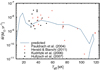 |
Fig. 4 Predicted mass-loss rate as a function of stellar temperature (solid blue line) in comparison with the observational results of Herald & Bianchi (2011) based on a UV analysis, the observational results of Kudritzki et al. (2006) and Hultzsch et al. (2007) based on an optical analysis, and the predictions of Pauldrach et al. (2004). |
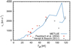 |
Fig. 5 Predicted terminal velocity as a function of stellar temperature (solid blue line) in comparison with observational results. |
Parameters of CSPNe with reliable distances.
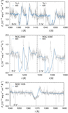 |
Fig. 6 Comparison of predicted spectra from the grid in Table 2 and IUE spectra of selected CSPNe. The predicted spectra were scaled to fit the continuum. Upper panel: Tc1 (central star HD 161044) and IUE spectrum SWP 42675. Middle panel: NGC 2392 and IUE spectrum SWP 19889. Bottom panel: NGC 1535 and IUE spectrum SWP 10821. |
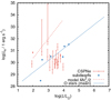 |
Fig. 7 Relation between observed X-ray luminosities and bolometric luminosities for CSPNe (Montez et al. 2015) and subdwarfs (Montez et al. 2010; La Palombara et al. 2012, 2014, 2015; Mereghetti et al. 2013). We overplotted the mean relation for O stars (Nazé 2009, blue solid line) and the wind kinetic energy loss per unit of time (red dashed line; derived using v∞ = 1000 km s−1 and mass-loss rate from Eq. (1) for T = 100 kK). |
5 Influence of metallicity
Hot star winds are driven by a radiative force due to heavier elements; consequently, the radiative force is sensitive to metallicity. Our calculations assumed solar chemical composition, which might not be realistic in many cases. The chemical composition of CSPNe partly reflects the composition of the interstellar medium, which can be nonsolar depending on the environment. Massive stars with an initial mass that is higher than about 1.2 M⊙ experience third dredge-up (Gallino et al. 2004), affecting the abundance of CNO elements and enriching the abundance of s-process elements at the expense of iron (Iben 1975).
We calculated additional wind models with an overabundance (Z = 3 Z⊙) and underabundance (Z = Z⊙∕3) of heavier elements. These might describe the influence of the dredge-up phase and the initially metal-poor environment, respectively. The resulting parameters of the models with nonsolar chemical composition are given in Table 7. On average, the wind mass-loss rate increases with metallicity as  , which is included in Eq. (1). The wind mass-loss rate is more sensitive to the metallicity for low mass-loss rates Ṁ < 10−9 M⊙ yr−1 at which the wind is typically driven by a few optically thick lines and, therefore, a small change in metallicity may cause a large change in the mass-loss rate.
6 Influence of clumping
We assumedspherically symmetric and stationary winds in our study. In reality, stellar winds are far from this assumption. It is generally considered that inhomogeneities on a small-scale (clumping) have the most significant effect on the wind structure. Clumping in hot star winds influences the ionization equilibrium (Hamann & Koesterke 1998; Bouret et al. 2003; Martins et al. 2005b; Puls at al. 2006) and the radiative transfer in the case of optically thick clumps either in continuum (Feldmeier et al. 2003)or in lines (Oskinova et al. 2007; Sundqvist et al. 2010, 2011; Šurlan et al. 2012, 2013). The origin of clumping is likely the line-driven wind instability (Lucy & Solomon 1970; Owocki & Rybicki 1984; Feldmeier & Thomas 2017), which may amplify the photospheric perturbations seeded by subsurface turbulent motions (Feldmeier et al. 1997; Cantiello & Braithwaite 2011; Jiang et al. 2015) or which may be self-initiated in the wind (Sundqvist et al. 2018).
In hot star winds, clumping affects not only the wind empirical characteristics, but also wind parameters. Optically thin clumping leads to an increase in the predicted mass-loss rates (Muijres et al. 2011; Krtička et al. 2018), which is in contrast to their influence on the empirical mass-loss rates. On the other hand, optically thick clumps counteract this effect. This has been found in a flow with a smooth velocity profile (Muijres et al. 2011) and the effect of optically thick clumps on the ionization structure in the wind with a nonmonotonic velocity profile (Sundqvist & Puls 2018) would also likely lead to the same result.
We included clumping into our wind models (for details see Krtička et al. 2018) assuming optically thin clumps. The clumping is parameterized by a clumping factor  , where the angle brackets denote the average over volume. Always Cc ≥ 1, and Cc = 1 corresponds to a smooth flow. We adopted the empirical radial clumping stratification from Najarro et al. (2009)
 (4)
(4)
which gives Cc(r) in terms of the radial wind velocity v(r). For our calculations, we inserted the radial velocity from the models without clumping into Eq. (4). Here, C1 is the clumping factor that is close to the star and the velocity C2 determines the location of the onset of clumping. Najarro et al. (2009) introduced additional constants C3 and C4 to account for the decrease of clumping in outer regions of dense winds (Puls at al. 2006). We neglected this effect because we are mostly concerned with the behavior of the wind that is close to the star. As a result, the formula becomes similar to what was used by Bouret et al. (2012), for example. Motivated by typical values derived in Najarro et al. (2009), we assume C1 = 10 and two values of C2, namely C2 = 100 km s−1 and C2 = 300 km s−1, for which the empirical Hα mass-loss rates of O stars agree with observations (Krtička & Kubát 2017). This gives a slightly higher value of the clumping factor than what was found from CSPN spectroscopy, which is about Cc ≈ 4 (Kudritzki et al. 2006; Hoffmann et al. 2016).
Wind parameters that were calculated with inclusion of clumping are given in Table 8 in comparison with the parameters derived for smooth winds (Cc = 1). In general, with increasing clumping, the rate of processes that depend on the square of the density also increases. Consequently, wind becomes less ionized and the mass-loss rate increases because ions in the lower degree of ionization accelerate wind more efficiently (Muijres et al. 2011). The effect is weaker for a higher value of C2 because with the increasing onset of clumping, the radiative force becomes less affected in the region close to the star where the mass-loss rate is determined. In exceptional cases, the mass-loss rate may decrease due to clumping. This happens when the lower ions are able to drive the wind less efficiently. For example, in the case of the T116 model, the clumping leads to a change in the dominant ionization stage of magnesium from Mg VII to Mg VI, which accelerates the wind less efficiently, thereby leading to a lower mass-loss rate (see Table 8).
Typically, the increase in the mass-loss rate is weaker than the dependence  derived for O stars (Muijres et al. 2011; Krtička et al. 2018). In a present sample, the mass loss rate typically varies as
  . The reason for this weaker dependence on clumping compared to O stars is most likely a lower contribution of iron lines to the radiative driving. The CSPN winds are mostly driven by elements that are lighter than iron. These elements effectively have a lower number of lines than iron, but these lines are significantly optically thick and they stay optically thick even after the change in ionization due to clumping. Because the radiative force due to optically thick lines is related to their number and not to the number density of corresponding levels, the radiative force only varies weakly with clumping.
Some models deviate more significantly from the mean incr- ease in the mass-loss rate with clumping. The model T23 with Cc = 1 (i.e., for a smooth wind without clumping) shows an increased mass-loss rate due to the commencing effect of the bistability jump. With clumping, the fraction of Fe III becomes even larger and the increase in the mass-loss rate with respect to the unclumped model is more significant than for other models. The influence of clumping is also stronger for winds at low mass-loss rates, which are typically given by a few lines and which are sensitive to a small change in the radiative force.
The model T18 is only very weakly sensitive to clumping. If this is also true for B supergiants, then this effect can partly explain the discrepancy (Crowther et al. 2006; Markova & Puls 2008; Haucke et al. 2018) between theoretical and empirical mass-loss rates for these stars in the region of the bistability jump. The same level of clumping at both sides of the jump would then lead to a larger increase in the mass-loss rate at the hot side of the jump, improving the agreement between theory and observation. The influence of clumping on the radiative transfer in the optically thick Hα line (Petrov et al. 2014) or different growth rates of instabilities (Driessen et al. 2019) can also contribute to explain the discrepancy.
Predicted wind parameters for individual metallicities.
Predicted wind parameters for different clumping.
7 Discussion
7.1 Influence of the magnetic field
White dwarfs, which are the descendants of central stars of planetary nebulae, are found to be magnetic (see Kawka 2018, for a review) with surface field strengths ranging from a few kilogauss up to about 1000 MG (e.g., Valyavin et al. 2006; Kawka & Vennes 2011; Landstreet et al. 2016). From this, we can expect strong surface magnetic fields, even in CSPNe. However, the observationsshow that this is not the case, placing the upper limit of the magnetic field strength to about 100 G (Jordan et al. 2012; Asensio Ramos et al. 2014; Leone et al. 2014; Steffen et al. 2014). This might pose problems for the models describing shapes of some planetary nebulae by magnetic fields (Aller 1958; Chvojková 1964; Chevalier & Luo 1994; García-Segura et al. 2005). On the other hand, the detection of few G fields in post-AGB stars (Sabin et al. 2015) shows that the magnetic fields with strength of the order 10 G may still be present in CSPN. In such a case, it is likely that the fields are frozen in the stellar plasma (similar to presumable fossil fields in hot main-sequence magnetic stars) and that the fields are stable over the CSPN lifetime. We discuss the effect of such fields on line driven winds.
The effect of the magnetic field is given by the ratio of the magnetic field density and the wind kinetic energy density:  . With a wind mass-loss rate of Ṁ = 4πr2ρv and by replacing B = Beq with the equatorial field strength, r = R* with the stellar radius, and v = v∞ with the terminal velocity, we derive
 (5)
(5)
which is the wind magnetic confinement parameter (ud-Doula & Owocki 2002). For weak confinement, η* ≲ 1, the wind energy density dominates over the magnetic field energy density and the wind speed is higher than the Alfvén velocity. The magnetic field opens up and the wind flows radially. For strong confinement, η* ≳ 1, the magnetic field energy density dominates over the wind energy density. Wind is trapped by the magnetic field and collision of wind flowfrom opposite footpoints of magnetic loops leads to magnetically confined wind shocks (Babel & Montmerle 1997).
In rewriting Eq. (5) in terms of typical parameters of CSPNe, we derive
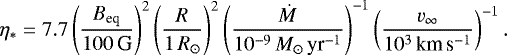 (6)
(6)
Consequently, even the magnetic field with strength that evades detection on the order of 10 G can still significantly affect the stellar wind especially in early post-AGB evolutionary stages with a large radius or in later phases with a low mass-loss rate.
The case of strong confinement η*≳ 1 leads to wind quenching (e.g., Petit et al. 2017). One can distinguish between two types of loops, closed and open ones. Within a closed loop, the wind speed is always lower than the Alfvén speed and wind confined within a closed loop never leaves the star (Babel & Montmerle 1997). The wind velocity at the apex of the last closed loop is just equal to the Alfvén speed. The wind only leaves the star on open loops on which the wind velocity exceeds the Alfvén speed at some point. Because the open loops cover just a fraction of the stellar surface, thisleads to a reduction in the mass-loss rate, that is, to the wind quenching. Assuming a dipolar field r = Rapex sin2θ, where Rapex is the apex radius and θ is the colatitude, equating Rapex = RA gives the magnetic field that is open for θ < θA, given by (ud-Doula & Owocki 2002)
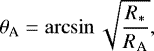 (7)
(7)
where  is the Alfvén radius (ud-Doula et al. 2008). Numerical simulations (ud-Doula et al. 2008) give a slightly lower maximum radius of a closed magnetic loop as Rc ≈ R* + 0.7(RA − R*). In the case of strong confinement, the wind only leaves the star in the direction of magnetic poles for angles θ < θA, forming a jet-like structure. The wind, therefore, only interacts with material from previous evolutionary stages in two opposite directions. This could possibly lead to a bipolar structure of some planetary nebulae (e.g., Kohoutek 1982; Lago & Costa 2016; Rechy-García et al. 2017).
Mass-loss via magnetised stellar wind also leads to the angular momentum loss and to the rotational braking (e.g., Soker 2006). The spin-down time depends on the stellar and wind parameters, on the magnetic field strength, and on the moment of inertia constant k (ud-Doula et al. 2009). To obtain a rough estimate of the moment of inertia constant k, which is not available from the Vassiliadis & Wood (1994) models, we used the MESA evolutionary code (Paxton et al. 2011, 2013). We let a star with an initial mass of 1 M⊙ evolve until the white dwarfs stage with a final mass of 0.52 M⊙. The moment of inertia constant k = 3.3 × 10⁻⁵ was derived from a model corresponding to a CSPN star with Teff = 15 kK. For typical stellar and wind parameters of CSPNe, Eq. (25) in ud-Doula et al. (2009) gives the spin-down time of about 103 yr for 100 G magnetic field strength. This is an order of magnitude shorter than the typical CSPN life-time (Miller Bertolami 2016). Consequently, magnetised CSPN significantly brake down their rotation, providing an additional explanation for low rotational velocities of white dwarfs (Hermes et al. 2017).
Magnetic braking at the top of the white dwarf cooling se- quence can explain extremely long rotational periods observed in some strongly magnetised white dwarfs (Bagnulo & Landstreet 2019). With k = 0.12, which was derived for the hot white dwarf stage of the MESA evolutionary track discussed in a previous paragraph, with a typical mass-loss rate of 10−10 M⊙ yr−1, and with B = 100 MG, the spindown time is about 104 yr (ud-Doula et al. 2009), which is a few orders of magnitude shorter than the white dwarf cooling timescale.
Magnetic field only influences the mass-loss via its channeling along the magnetic field lines, while the influence of the Zeeman effect is negligible for magnetic fields that are weaker than about 105 G (Krtička 2018). On the other hand, some white dwarfs show a magnetic field that is stronger than this limit. Consequently, for hot white dwarfs with extremely strong magnetic fields, the line splitting due to the Zeeman effect might affect the line force and the mass-loss rate.
7.2 Shaping a planetary nebulae
Much effort was put into understanding the shapes of planetary nebulae since the proposition of Kwok et al. (1978) that these nebulae originate from the collision of fast weak wind with slow dense outflow coming from previous evolutionary phases. It is typically assumed that the AGB wind is the main culprit of the aspherical shape of many planetary nebulae, but the wind of CSPNe may also play its role. There are several effects that lead to departures of the CSPN wind structure from spherical symmetry and which may therefore cause asymmetry of planetary nebulae.
Magnetic fields have long been suspected to cause the bipolar shape of planetary nebulae (e.g., Chevalier & Luo 1994; García-Segura et al. 2005). We find that the magnetic fields with strengths on the order of 10 G that evade the detection may still have a significant impact on the wind (see Eq. (6)). A magnetic field with η* ≳ 1 (introduced in Eq. (5)) confines the wind into a form of narrow outflow with an opening angle given by the Alfvén radius Eq. (7). The magnetic field axis may likely be tilted with respect to the rotational axis as in magnetic main-sequence stars (see Wade & Neiner 2018, for a recent review). In such a case, the narrow outflow (jet) precesses with the rotational period. Such precessing jets were inferred from observations (Sahai et al. 2005). In the case of fast rotation, the rotational signature is likely smeared out and the precessing jets may create just bipolar lobes.
Fast rotation is another mechanism that can potentially lead to the winds that are not spherically symmetric. As a result of fast rotation, the stellar equator becomes cooler, leading to weaker flow in the equatorial region than in the polar region (Owocki et al. 1996). Such effects are important when the rotational velocity is close to the critical rotational speed 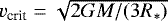 , which is vcrit = 60 km s−1 for T10 model, but is vcrit = 330 km s−1 for T55 model, which roughly corresponds to typical CSPN parameters. Due to a huge increase in the moment of inertia in late phases of stellar evolution, angular momentum loss, and efficient coupling between the core and envelope (Suijs et al. 2008; García-Segura et al. 2014), the stellar remnants are predicted to rotate very slowly. Even magnetic torques are needed to reproduce the observed rotational velocities of white dwarfs, which are typically rather slow (Kawaler 2004). Consequently, even CSPNe with extreme rotational speeds rotate at a small fraction of the critical velocity (Prinja et al. 2012) and thus shaping of planetary nebula by rotating post-AGB winds is unlikely.
Another effect that can influence the structure of planetary nebulae is the bistability jump around Teff = 20 kK (see Fig. 4). During the post-AGB evolution, the mass-loss rate decreases by a factor of about 8 and the wind terminal velocity increases by a factor of roughly 2 around the bistability jump. Therefore, after the star passes through the bistability jump, the fast weak wind overtakes the slow dense wind, resembling the situation just after leaving the AGB phase. This could possibly lead to the creation of an additional inner shell of planetary nebulae.
7.3 Wind limits
The wind mass-loss rate is on the order of 10−9 M⊙ yr−1 during the post-AGB evolutionary phase with constant luminosity. The mass-loss rate starts to significantly decrease when the star turns right in the HR diagram and settles on the white dwarf cooling track (Fig. 4). For our selected evolutionary track, there is a wind limit at about 105 kK below whichthere are no homogeneous (i.e., hydrogen and helium dominated) stellar winds (see Table 2). The location of the wind limit nicely agrees with results of Unglaub & Bues (2000), who found the wind limit at about 120 kK for solar abundance stars with log g = 7 (see their Fig. 1).
The location of the wind limit was derived from additional models with a fixed hydrodynamical structure, where we compared the radiative force with the gravity for several different mass-loss rates between 10−16 M⊙ yr−1 − 10−10 M⊙ yr−1 (for details see Krtička 2014). In all models descending on the white dwarf cooling track with Teff< 105 kK and log (L∕L⊙) < 2.4, the radiative force was lower than the gravity force. This means that the radiative force is not able to drive a homogeneous wind and that there is no (hydrogen or helium dominated) wind below Teff< 105 kK.
The existence of the wind limit around Teff ≈ 105 kK is supportedby the observation of hot white dwarfs with near-solar chemical composition (Werner et al. 2017, 2018, 2019). Despite their high gravity, the stellar wind possibly prevents the gravitational settling (Unglaub & Bues 2000). This region in the HR diagram with fading wind where the gravity and radiative force compete can be theoretically appealing. Similar processes as in classical chemically peculiar stars, including rotationally modulated spectroscopic and photometric variability (e.g., Kochukhov et al. 2014; Prvák et al. 2015), may also appear in hot white dwarfs.
Unglaub & Bues (1998, 2000) showed that the wind mass-loss rate limit that prevents abundance stratification is about 10−12 M⊙ yr−1. From Table 2, it follows that the predicted division between homogeneous and stratified atmospheres lies at about 110 kK, which is in reasonable agreement with observations. An exact location of this boundary is uncertain due to a large sensitivity of the wind mass-loss rate on the stellar parameters, such as the effective temperature and metallicity (see, e.g., Table 7).
To better understand the influence of metallicity on the location of the wind limit, we performed additional wind tests with a factor of 10 higher abundance of iron and silicon. This leads to a shift in the wind limit of 5–100 kK in the models with overabundant iron and to a shift of about 15–89 kK in the models with overabundant silicon. The location of the wind limit is also significantly different in He-rich stars and in PG 1159 stars (Unglaub & Bues 2000).
There is a possibility to launch an outflow even below the wind limit. Such an outflow is not chemically homogeneous and consists of individual radiatively accelerated metallic ions (Babel 1995).
There is a relatively strong line driven wind, even for the coolest star in our sample, with Teff = 10 kK. This indicates that even cooler star likely have line-driven winds. This is consistent with the observation of P Cygni line profiles in the B-type post-AGB stars (Sarkar et al. 2012).
7.4 Effects of a multicomponent flow and frictional heating
Hot star winds are mostly driven by the radiative force acting on heavier elements, while the radiative force on hydrogen and helium is negligible. The momentum acquired from radiation is transferred by Coulomb collisions to hydrogen and helium, which constitute the bulk of the wind. In dense winds, the momentum transfer is very efficient; consequently, dense winds can be treated as a one-component flow assuming equal velocities of all ions (Castor et al. 1976). However, in low-density winds, the Coulomb collisions are less efficient, which leads to the frictional heating and to decoupling of individual components (Springmann & Pauldrach 1992; Krtička & Kubát 2001; Owocki & Puls 2002; Votruba et al. 2007; Unglaub 2008).
The effects of a multicomponent flow become important when the star appears at the white dwarf cooling track, decreasing its luminosity and mass-loss rate (Krtička & Kubát 2005). Their importance can be estimated from the value of the relative velocity difference xhp (Eq. (18) in Krtička 2006) between a given element h and protons. When the velocity difference is low, xhp ≲ 0.1, the multicomponent effects are unimportant, while for xhp ≳ 0.1, friction may heat the wind, and for xhp ≳ 1 the element h decouples.
We calculated the relative velocity difference xhp according toKrtička (2006) for all heavier elements. In a given wind model, the relative velocity difference increases with the radius due to decreasing density and reaches maximum in the outer parts of the wind. Our calculations show that for high luminosities log (L∕L⊙) ≳ 2.9, the wind density is so high that the maximum nondimensional velocity difference is low, xhp< 0.1, and therefore the flow can be considered as a one-component one. For lower luminosities, log (L∕L⊙) ≲ 2.5 (in the model T105), the maximum nondimensional velocity difference is higher, xhp> 0.1; consequently, the wind may be frictionally heated or the components may decouple. The elements that may decouple are those which significantly contribute to the radiative driving, which are Ne, Mg, and Si for parameters corresponding to the T105 model. The decoupling affects the wind terminal velocity and may even reduce the bulk mass-loss rate if it appears close to the critical point, where the wind velocity is equal to the speed of the Abbott (1980) radiative-acoustic waves (see also Feldmeier et al. 2008).
The frictionally heated winds were connected with the presence of ultrahigh-excitation absorption lines in the spectra of hot white dwarfs (Werner et al. 1995, 2018). In such a case, the optical depth of a given line should be close to one to cause a considerable absorption. In neglecting the finite cone effects and the population of the upper level, the condition for unity Sobolev line optical depth in a supersonic wind (Castor 1970) reads as
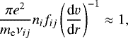 (8)
(8)
where ni is the number density of atoms in the lower level of a corresponding line transition with frequency νij and oscillator strength fij and where d v∕dr is the velocity gradient. Assuming fij ≈ 1 and approximating dv∕dr ≈ v∞∕R*, the minimum mass-loss rate needed to cause a considerable absorption is
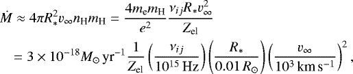 (9)
(9)
where Zel is the ratio of number densities of a given element and hydrogen. This shows that for CNO elements with Zel ≈ 10−3, the absorption line profiles can be observed down to the bulk mass-loss rates of the order 10−14 M⊙ yr−1 in hot white dwarfs. Moreover, the wind with velocity on the order of 103 km s−1 has a high enough kinetic energy that just part of it is able to heat the wind to the temperatures required to generate ultrahigh-excitation lines. Therefore, the presence of ultrahigh-excitation absorption lines can be possibly explained by the frictionally heated wind.
8 Conclusions
We studied line-driven winds of white dwarf progenitors along their evolution between the AGB stage and the top of the white dwarf cooling track. We calculated global wind models for individual stellar parameters obtained from evolutionary models with a CSPN mass of 0.569 M⊙ and predicted wind structure, including wind mass-loss rates and terminal velocities. We compared derived results with observations.
Line driven winds are initiated very early after leaving the AGB phase and appear, at the latest, for Teff ≈ 10 kK (but most likely even earlier). Because the wind mass-loss rate mostly depends on the stellar luminosity, which is nearly constant along the evolutionary track, the mass-loss rate does not vary significantly during most of the CSPN evolution and is on the order of 10−9 M⊙ yr−1. This nicely agrees with observations. We fit our resulting mass-loss rate as a function of stellar effective temperature and provided corresponding scalings that account for different luminosities and metallicities. Line-driven winds fade out at the white dwarf cooling track for temperatures of about 105 kK for solar metallicity composition. Possibly only metallic winds exist below this limit.
Two features interfere with an otherwise nearly constant mass-loss rate along the post-AGB evolutionary track. A bistability jump at around Teff ≈ 20 kK due to the change in dominant iron ion from Fe III to Fe IV leads to a decrease in the mass-loss rate by a factor of about 8 and to an increase in the terminal velocity by a factor of roughly 2 (during the evolution). At about Teff = 45 kK, additional broad and weak maximum of mass-loss rates appears, which we interpreted as a result of an increase in the far-UV radiative flux.
Because the post-AGB evolution proceeds at roughly constant luminosity, the stellar radius decreases with increasing effective temperature. This and the proportionality between the escape speed and the wind terminal velocity cause the wind terminal velocity to increase during the post-AGB evolution. This nicely agrees with observed terminal velocities. The predicted and observational values also agree, although we argue that this could be partly a consequence of adopted luminosities, which are slightly lower than those derived from observations of typical CSPNe and from updated evolutionary models (Miller Bertolami 2016). Therefore, as in the case of O stars (Krtička & Kubát 2017), our models slightly underpredict the wind terminal velocities, which could be caused by radial variations of clumping or by X-ray irradiation. As the winds start to fade out close to the white dwarf cooling track, the wind terminal velocities also decrease.
We calculated the number of ionizing photons and compared the values with results of plane-parallel models. As a result, it follows that the number of H I ionizing photons can be derived from plane-parallel photospheric models for Teff≳ 40 kK and that the plane-parallel models predict a reliable number of He I ionizing photons for Teff≳ 50 kK. For cooler stars, the effects of spherical symmetry and envelope extension are so strong that the number of ionizing photons are not reliably predicted from plane–parallel models. On the other hand, wind absorption above the He II ionization jump is so strong that the plane-parallel models never predict the correct number of He II ionizing photons for any star with wind and even results of spherical models are sensitive to model assumptions.
We discuss how the wind properties can contribute to the shaping of planetary nebula. The bistability jump can lead to the appearance of an additional shell of planetary nebula. Magnetic fields with strengths that are close to their observational upper limits are still powerful enough to channel the wind along the field lines and to affect the shaping of planetary nebulae (Steffen et al. 2014)and the rotational evolution of CSPNe.
Our models provide reliable wind parameters that can be used in post-AGB evolutionary calculations or in the studies of planetary nebulae.
Acknowledgements
This research was supported by grant GA ČR 18-05665S. Computational resources were provided by the CESNET LM2015042 and the CERIT Scientific Cloud LM2015085, provided under the programme “Projects of Large Research, Development, and Innovations Infrastructures”. The Astronomical Institute Ondřejov is supported by a project RVO:67985815 of the Academy of Sciences of the Czech Republic.
References
- Abbott, D. C. 1980, ApJ, 242, 1183 [NASA ADS] [CrossRef] [Google Scholar]
- Aller, L. H. 1958, AJ, 63, 47 [NASA ADS] [CrossRef] [Google Scholar]
- Asensio Ramos, A., Martínez González, M. J., Manso Sainz, R., Corradi, R. L. M., & Leone, F. 2014, ApJ, 787, 111 [NASA ADS] [CrossRef] [Google Scholar]
- Asplund, M., Grevesse, N., Sauval, A. J., & Scott, P. 2009, ARA&A, 47, 481 [NASA ADS] [CrossRef] [Google Scholar]
- Babel, J. 1995, A&A, 301, 823 [Google Scholar]
- Babel, J., & Montmerle, T. 1997, A&A, 323, 121 [NASA ADS] [Google Scholar]
- Bagnulo, S., & Landstreet, J. D. 2019, MNRAS, 486, 4655 [NASA ADS] [CrossRef] [Google Scholar]
- Bautista, M. A., & Pradhan, A. K. 1997, A&AS, 126, 365 [NASA ADS] [CrossRef] [EDP Sciences] [Google Scholar]
- Bloecker, T. 1995, A&A, 299, 755 [NASA ADS] [Google Scholar]
- Bouret, J.-C., Lanz, T., Hillier, D. J., et al. 2003, ApJ, 595, 1182 [NASA ADS] [CrossRef] [Google Scholar]
- Bouret, J.-C., Hillier, D. J., Lanz, T., & Fullerton, A. W. 2012, A&A, 544, A6 [NASA ADS] [CrossRef] [EDP Sciences] [Google Scholar]
- Butler, K., Mendoza, C., & Zeippen, C. J. 1993, J. Phys. B. 26, 4409 [NASA ADS] [CrossRef] [Google Scholar]
- Cantiello, M., & Braithwaite, J. 2011, A&A, 534, A140 [NASA ADS] [CrossRef] [EDP Sciences] [Google Scholar]
- Castor, J. I. 1970, MNRAS, 149, 111 [NASA ADS] [Google Scholar]
- Castor, J. I., Abbott D. C., & Klein, R. I. 1975, ApJ, 195, 157 [NASA ADS] [CrossRef] [Google Scholar]
- Castor, J. I., Abbott, D. C., & Klein, R. I. 1976, Physique Des Mouvements Dans Les Atmosphères Stellaires, eds. R. Cayrel, & M. Sternberg (Paris: CNRS), 363 [Google Scholar]
- Chen, G. X., & Pradhan, A. K. 1999, A&AS, 136, 395 [NASA ADS] [CrossRef] [EDP Sciences] [Google Scholar]
- Chevalier, R. A., & Luo, D. 1994, ApJ, 421, 225 [NASA ADS] [CrossRef] [Google Scholar]
- Chu, Y.-H., Guerrero, M. A., Gruendl, R. A., Williams, R. M., & Kaler, J. B. 2001, ApJ, 553, L69 [NASA ADS] [CrossRef] [Google Scholar]
- Chvojková, E. 1964, Bull. Astron. Inst. Czechoslov., 15, 241 [NASA ADS] [Google Scholar]
- Crowther, P. A., Lennon, D. J., & Walborn, N. R. 2006, A&A, 446, 279 [NASA ADS] [CrossRef] [EDP Sciences] [Google Scholar]
- Driessen, F. A., Sundqvist, J. O., & Kee, N. D. 2019, A&A, 631, A172 [NASA ADS] [CrossRef] [EDP Sciences] [Google Scholar]
- Falcon, R. E., Winget, D. E., Montgomery, M. H., & Williams, K. A. 2010, ApJ, 712, 585 [NASA ADS] [CrossRef] [Google Scholar]
- Feldmeier, A., & Thomas, T. 2017, MNRAS, 469, 3102 [NASA ADS] [CrossRef] [Google Scholar]
- Feldmeier, A., Puls, J., & Pauldrach, A. W. A. 1997, A&A, 322, 878 [NASA ADS] [Google Scholar]
- Feldmeier, A., Oskinova, L., & Hamann, W.-R. 2003, A&A, 403, 217 [NASA ADS] [CrossRef] [EDP Sciences] [Google Scholar]
- Feldmeier, A., Rätzel, D., & Owocki, S. P. 2008, ApJ, 679, 704 [NASA ADS] [CrossRef] [Google Scholar]
- Fernley J. A., Taylor K. T., & Seaton, M. J. 1987, J. Phys. B, 20, 6457 [NASA ADS] [CrossRef] [Google Scholar]
- Freeman, M., Montez, R., Jr. Kastner, J. H., et al. 2014, ApJ, 794, 99 [NASA ADS] [CrossRef] [Google Scholar]
- Gaia Collaboration (Prusti, T., et al.) 2016, A&A, 595, A1 [NASA ADS] [CrossRef] [EDP Sciences] [Google Scholar]
- Gaia Collaboration (Brown, A. G. A., et al.) 2018, A&A, 616, A1 [NASA ADS] [CrossRef] [EDP Sciences] [Google Scholar]
- Gallino, R., Arnone, E., Pignatari, M., & Straniero, O. 2004, Mem. Soc. Astron. It., 75, 700 [NASA ADS] [Google Scholar]
- García-Segura, G., López, J. A., & Franco, J. 2005, ApJ, 618, 919 [NASA ADS] [CrossRef] [Google Scholar]
- García-Segura, G., Villaver, E., Langer, N., Yoon, S.-C., & Manchado, A. 2014, ApJ, 783, 74 [NASA ADS] [CrossRef] [Google Scholar]
- González-Santamaría, I., Manteiga, M., Manchado, A., et al. 2019, A&A, 630, A150 [NASA ADS] [CrossRef] [EDP Sciences] [Google Scholar]
- Green, G. M., Schlafly, E. F., Finkbeiner, D., et al. 2018, MNRAS, 478, 651 [NASA ADS] [CrossRef] [Google Scholar]
- Guerrero, M. A. 2006, IAU Symp., 234, 153 [NASA ADS] [CrossRef] [Google Scholar]
- Hamann, W.-R., & Koesterke, L. 1998, A&A, 335, 1003 [NASA ADS] [Google Scholar]
- Haucke, M., Cidale, L. S., Venero, R. O. J., et al. 2018, A&A, 614, A91 [NASA ADS] [CrossRef] [EDP Sciences] [Google Scholar]
- Heller, R., Jacob, R., Schönberner, D., & Steffen, M. 2018, A&A, 620, A98 [NASA ADS] [CrossRef] [EDP Sciences] [Google Scholar]
- Herald, J. E., & Bianchi, L. 2011, MNRAS, 417, 2440 [NASA ADS] [CrossRef] [Google Scholar]
- Hermes, J. J., Gänsicke, B. T., Kawaler, S. D., et al. 2017, ApJS, 232, 23 [NASA ADS] [CrossRef] [Google Scholar]
- Herrero, A., Kudritzki R. P., Vilchez, J. M., et al. 1992, A&A, 261, 209 [NASA ADS] [Google Scholar]
- Herrmann, K. A., Ciardullo, R., Feldmeier, J. J., & Vinciguerra, M. 2008, ApJ, 683, 630 [NASA ADS] [CrossRef] [Google Scholar]
- Hoffmann, T. L., Pauldrach, A. W. A., & Kaschinski, C. B. 2016, A&A, 592, A158 [NASA ADS] [CrossRef] [EDP Sciences] [Google Scholar]
- Hultzsch, P. J.N., Puls, J., Méndez, R. H., et al. 2007, A&A, 467, 1253 [NASA ADS] [CrossRef] [EDP Sciences] [Google Scholar]
- Hummer, D. G., Berrington, K. A., Eissner, W., et al. 1993, A&A, 279, 298 [NASA ADS] [Google Scholar]
- Iben, I., Jr. 1975, ApJ, 196, 549 [NASA ADS] [CrossRef] [Google Scholar]
- Jiang, Y.-F., Cantiello, M., Bildsten, L., Quataert, E., & Blaes, O. 2015, ApJ, 813, 7 [NASA ADS] [CrossRef] [Google Scholar]
- Jordan, S., Bagnulo, S., Werner, K., & O’Toole, S. J. 2012, A&A, 542, A64 [NASA ADS] [CrossRef] [EDP Sciences] [Google Scholar]
- Kaschinski, C.B., Pauldrach, A. W. A., & Hoffmann, T. L. 2012, A&A, 542, A45 [NASA ADS] [CrossRef] [EDP Sciences] [Google Scholar]
- Kawaler, S. D. 2004, IAU Symp., 215, 561 [NASA ADS] [Google Scholar]
- Kawka, A. 2018, Contrib. Astron. Observ. Skalnaté Pleso, 48, 228 [NASA ADS] [Google Scholar]
- Kawka, A., & Vennes, S. 2011, A&A, 532, A7 [NASA ADS] [CrossRef] [EDP Sciences] [Google Scholar]
- Kleinman, S. J., Kepler, S. O., Koester, D., et al. 2013, ApJS, 204, 5 [NASA ADS] [CrossRef] [MathSciNet] [Google Scholar]
- Kochukhov, O., Lüftinger, T., Neiner, C., & Alecian, E. 2014, A&A, 565, A83 [NASA ADS] [CrossRef] [EDP Sciences] [Google Scholar]
- Koester, D. 1987, ApJ, 322, 852 [NASA ADS] [CrossRef] [Google Scholar]
- Kohoutek, L. 1982, A&A, 115, 420 [NASA ADS] [Google Scholar]
- Kramida, A., Ralchenko, Y., Reader, J., and NIST ASD Team 2015, NIST Atomic Spectra Database (ver. 5.3) [Google Scholar]
- Krtička, J. 2006, MNRAS, 367, 1282 [NASA ADS] [CrossRef] [Google Scholar]
- Krtička, J. 2018, A&A, 620, A176 [NASA ADS] [CrossRef] [EDP Sciences] [Google Scholar]
- Krtička, J. 2014, A&A, 564, A70 [NASA ADS] [CrossRef] [EDP Sciences] [Google Scholar]
- Krtička, J., & Kubát, J. 2001, A&A, 377, 155 [NASA ADS] [CrossRef] [EDP Sciences] [Google Scholar]
- Krtička, J., & Kubát, J. 2005, ASP Conf. Ser., 334, 337 [NASA ADS] [Google Scholar]
- Krtička, J., & Kubát, J. 2010, A&A, 519, A5 [NASA ADS] [CrossRef] [EDP Sciences] [Google Scholar]
- Krtička, J., & Kubát, J. 2017, A&A, 606, A31 [NASA ADS] [CrossRef] [EDP Sciences] [Google Scholar]
- Krtička, J., Kubát, J., & Krtičková, I. 2018, A&A, 620, A150 [NASA ADS] [CrossRef] [EDP Sciences] [Google Scholar]
- Kubát, J. 1996, A&A, 305, 255 [NASA ADS] [Google Scholar]
- Kubát, J. 1997, A&A, 323, 524 [NASA ADS] [Google Scholar]
- Kubát, J., Puls, J., & Pauldrach, A. W. A. 1999, A&A, 341, 587 [NASA ADS] [Google Scholar]
- Kudritzki, R. P., Urbaneja, M. A., & Puls, J. 2006, IAU Symp., 234, 119 [NASA ADS] [CrossRef] [Google Scholar]
- Kunasz, P. B., Hummer, D. G., & Mihalas, D. 1975, ApJ 202, 92 [NASA ADS] [CrossRef] [Google Scholar]
- Kupka, F., Piskunov, N. E., Ryabchikova, T. A., Stempels, H. C., & Weiss, W. W. 1999, A&AS, 138, 119 [NASA ADS] [CrossRef] [EDP Sciences] [MathSciNet] [PubMed] [Google Scholar]
- Kurucz, R. L. 1994, Kurucz CD-ROM 1 (Cambridge: SAO) [Google Scholar]
- Kwok, S. 2008, IAU Symp., 252, 197 [NASA ADS] [CrossRef] [Google Scholar]
- Kwok, S., Purton, C. R., & Fitzgerald, P. M. 1978, ApJ, 219, L125 [NASA ADS] [CrossRef] [Google Scholar]
- Lago, P. J. A.,& Costa, R. D. D. 2016, Rev. Mex. Astron. Astrofis., 52, 329 [NASA ADS] [Google Scholar]
- Lamers, H. J. G. L. M., Snow, T. P., & Lindholm, D. M. 1995, ApJ, 455, 269 [NASA ADS] [CrossRef] [Google Scholar]
- Landstreet, J. D., Bagnulo, S., Martin, A., & Valyavin, G. 2016, A&A, 591, A80 [NASA ADS] [CrossRef] [EDP Sciences] [Google Scholar]
- Lanz, T., & Hubeny, I. 2003, ApJS, 146, 417 [NASA ADS] [CrossRef] [Google Scholar]
- Lanz, T., & Hubeny, I. 2007, ApJS, 169, 83 [CrossRef] [Google Scholar]
- La Palombara, N., Mereghetti, S., Tiengo, A., & Esposito, P. 2012, ApJ, 750, L34 [NASA ADS] [CrossRef] [Google Scholar]
- La Palombara, N., Esposito, P., Mereghetti, S., & Tiengo, A. 2014, A&A, 566, A4 [NASA ADS] [CrossRef] [EDP Sciences] [Google Scholar]
- La Palombara, N., Esposito, P., Mereghetti, S., Novara, G., & Tiengo, A. 2015, A&A, 580, A56 [NASA ADS] [CrossRef] [EDP Sciences] [Google Scholar]
- Leone, F., Corradi, R. L. M., Martínez González, M. J., Asensio Ramos, A., & Manso Sainz, R. 2014, A&A, 563, A43 [NASA ADS] [CrossRef] [EDP Sciences] [Google Scholar]
- Lucy, L. B., & Solomon, P. M. 1970, ApJ, 159, 879 [NASA ADS] [CrossRef] [Google Scholar]
- Luo, D., & Pradhan, A. K. 1989, J. Phys. B, 22, 3377 [NASA ADS] [CrossRef] [Google Scholar]
- Markova, N., & Puls, J. 2008, A&A, 478, 823 [NASA ADS] [CrossRef] [EDP Sciences] [Google Scholar]
- Markova, N., Puls, J., & Langer, N. 2018, A&A, 613, A12 [NASA ADS] [CrossRef] [EDP Sciences] [Google Scholar]
- Martins, F., Schaerer, D., & Hillier, D. J. 2005a, A&A, 436, 1049 [NASA ADS] [CrossRef] [EDP Sciences] [Google Scholar]
- Martins, F., Schaerer, D., Hillier, D. J., et al. 2005b, A&A, 441, 735 [NASA ADS] [CrossRef] [EDP Sciences] [Google Scholar]
- Mendez, R. H., Kudritzki, R. P., Herrero, A., Husfeld, D., & Groth, H. G. 1988, A&A, 190, 113 [NASA ADS] [Google Scholar]
- Mereghetti, S., La Palombara, N., Tiengo, A., et al. 2013, A&A, 553, A46 [NASA ADS] [CrossRef] [EDP Sciences] [Google Scholar]
- Mihalas, D., Kunasz, P. B., & Hummer, D. G. 1975, ApJ, 202, 465 [NASA ADS] [CrossRef] [Google Scholar]
- Milingo, J. B., Kwitter, K. B., Henry, R. B. C., & Souza, S. P. 2010, ApJ, 711, 619 [NASA ADS] [CrossRef] [Google Scholar]
- Miller Bertolami, M. M. 2016, A&A, 588, A25 [NASA ADS] [CrossRef] [EDP Sciences] [Google Scholar]
- Mokiem, M. R., Martín-Hernández, N. L., Lenorzer, A., de Koter, A., & Tielens, A. G. G. M. 2004, A&A, 419, 319 [NASA ADS] [CrossRef] [EDP Sciences] [Google Scholar]
- Montez, R., Jr. De Marco, O., Kastner, J. H., & Chu, Y.-H. 2010, ApJ, 721, 1820 [NASA ADS] [CrossRef] [Google Scholar]
- Montez, R., Jr. Kastner, J. H., Balick, B., et al. 2015, ApJ, 800, 8 [NASA ADS] [CrossRef] [Google Scholar]
- Muijres L., de Koter A., Vink J., et al. 2011, A&A, 526, A32 [Google Scholar]
- Nahar, S. N., & Pradhan, A. K. 1993, J. Phys. B, 26, 1109 [NASA ADS] [CrossRef] [Google Scholar]
- Nahar, S. N., & Pradhan, A. K. 1994, J. Phys. B, 27, 429 [NASA ADS] [CrossRef] [Google Scholar]
- Nahar, S. N., & Pradhan, A. K. 2006, ApJS, 162, 417 [NASA ADS] [CrossRef] [Google Scholar]
- Najarro, F., Figer, D. F., Hillier, D. J., Geballe, T. R., & Kudritzki, R. P. 2009, ApJ, 691, 1816 [NASA ADS] [CrossRef] [Google Scholar]
- Nazé, Y. 2009, A&A, 506, 1055 [NASA ADS] [CrossRef] [EDP Sciences] [Google Scholar]
- Oskinova, L. M., Hamann W.-R., & Feldmeier, A. 2007, A&A, 476, 133 [Google Scholar]
- Owocki, S. P., & Puls, J. 2002, ApJ, 568, 965 [NASA ADS] [CrossRef] [Google Scholar]
- Owocki, S. P., & Rybicki, G. B. 1984, ApJ 284, 337 [NASA ADS] [CrossRef] [Google Scholar]
- Owocki, S. P., Cranmer, S. R., & Gayley, K. G. 1996, ApJ, 472, 115 [Google Scholar]
- Pauldrach, A. W. A., & Puls, J. 1990, A&A, 237, 409 [NASA ADS] [Google Scholar]
- Pauldrach, A., Puls, J., Kudritzki, R. P., Mendez, R. H., & Heap, S. R. 1988, A&A, 207, 123 [NASA ADS] [Google Scholar]
- Pauldrach, A. W. A., Hoffmann, T. L., & Lennon, M. 2001, A&A, 375, 161 [NASA ADS] [CrossRef] [EDP Sciences] [Google Scholar]
- Pauldrach, A. W. A., Hoffmann, T. L., & Méndez, R. H. 2004, A&A, 419, 1111 [NASA ADS] [CrossRef] [EDP Sciences] [Google Scholar]
- Paxton, B., Bildsten, L., Dotter, A., et al. 2011, ApJS, 192, 3 [Google Scholar]
- Paxton, B., Cantiello, M., Arras, P., et al. 2013, ApJS, 208, 4 [NASA ADS] [CrossRef] [Google Scholar]
- Peach, G., Saraph, H. E., & Seaton, M. J. 1988, J. Phys. B, 21, 3669 [NASA ADS] [CrossRef] [Google Scholar]
- Petit, V., Keszthelyi, Z., MacInnis, R., et al. 2017, MNRAS, 466, 1052 [NASA ADS] [CrossRef] [Google Scholar]
- Petrov, B., Vink, J. S., & Gräfener, G. 2014, A&A, 565, A62 [NASA ADS] [CrossRef] [EDP Sciences] [Google Scholar]
- Piskunov, N. E., Kupka, F., Ryabchikova, T. A., Weiss, W. W., & Jeffery, C. S. 1995, A&AS, 112, 525 [NASA ADS] [Google Scholar]
- Prinja, R. K., Massa, D. L., & Cantiello, M. 2012, ApJ, 759, L28 [NASA ADS] [CrossRef] [Google Scholar]
- Prvák, M., Liška J., Krtička J., Mikulášek Z., & Lüftinger, T. 2015, A&A, 584, A17 [NASA ADS] [CrossRef] [EDP Sciences] [Google Scholar]
- Puls, J., Urbaneja, M. A., Venero, R., et al. 2005, A&A, 435, 669 [NASA ADS] [CrossRef] [EDP Sciences] [Google Scholar]
- Puls, J., Markova N., Scuderi S., et al. 2006, A&A, 454, 625 [NASA ADS] [CrossRef] [EDP Sciences] [Google Scholar]
- Rechy-García, J. S., Velázquez, P. F., Pe na, M., & Raga, A. C. 2017, MNRAS, 464, 2318 [NASA ADS] [CrossRef] [Google Scholar]
- Richer, M. G.,& McCall, M. L. 2008, ApJ, 684, 1190 [NASA ADS] [CrossRef] [Google Scholar]
- Sabin, L., Wade, G. A., & Lèbre, A. 2015, MNRAS, 446, 1988 [NASA ADS] [CrossRef] [Google Scholar]
- Sahai, R., Le Mignant, D., Sánchez Contreras, C., Campbell, R. D., & Chaffee, F. H. 2005, ApJ, 622, L53 [NASA ADS] [CrossRef] [Google Scholar]
- Sander, A. A. C., Hamann, W.-R., Todt, H., et al. 2017, A&A, 603, A86 [NASA ADS] [CrossRef] [EDP Sciences] [Google Scholar]
- Sarkar, G., García-Hernández, D. A., Parthasarathy, M., et al. 2012, MNRAS, 421, 679 [NASA ADS] [Google Scholar]
- Sawey, P. M. J., & Berrington, K. A. 1992, J. Phys. B, 25, 1451 [NASA ADS] [CrossRef] [Google Scholar]
- Schönberner, D., Jacob, R., Steffen, M., et al. 2005, A&A, 431, 963 [NASA ADS] [CrossRef] [EDP Sciences] [Google Scholar]
- Scuderi, S., Panagia, N., Stanghellini, C., Trigilio, C., & Umana, G. 1998, A&A 332, 251 [NASA ADS] [Google Scholar]
- Seaton, M. J., Zeippen, C. J., Tully, J. A. et al. 1992, Rev. Mex. Astron. Astrofis., 23, 19 [NASA ADS] [EDP Sciences] [Google Scholar]
- Soker, N. 2006, PASP, 118, 260 [NASA ADS] [CrossRef] [Google Scholar]
- Springmann, U. W. E., & Pauldrach, A. W. A. 1992, A&A 262, 515 [NASA ADS] [Google Scholar]
- Stasińska, G., Gorny, S. K., & Tylenda, R. 1997, A&A, 327, 736 [NASA ADS] [Google Scholar]
- Stasińska, G., Richer, M. G., & McCall, M. L. 1998, A&A, 336, 667 [NASA ADS] [Google Scholar]
- Steffen, M., Hubrig, S., Todt, H., et al. 2014, A&A, 570, A88 [NASA ADS] [CrossRef] [EDP Sciences] [Google Scholar]
- Suijs, M. P. L., Langer, N., Poelarends, A.-J., et al. 2008, A&A, 481, L87 [NASA ADS] [CrossRef] [EDP Sciences] [Google Scholar]
- Sundqvist, J. O., & Puls, J. 2018, A&A, 619, A59 [NASA ADS] [CrossRef] [EDP Sciences] [Google Scholar]
- Sundqvist, J. O., Puls, J., & Feldmeier, A. 2010, A&A, 510, A11 [NASA ADS] [CrossRef] [EDP Sciences] [Google Scholar]
- Sundqvist, J. O., Puls, J., Feldmeier, A., & Owocki, S. P. 2011, A&A, 528, A6 [EDP Sciences] [Google Scholar]
- Sundqvist, J. O., Owocki, S. P., & Puls, J. 2018, A&A, 611, A17 [NASA ADS] [CrossRef] [EDP Sciences] [Google Scholar]
- Šurlan, B., Hamann W.-R., Kubát J., Oskinova L., & Feldmeier, A. 2012, A&A, 541, A37 [NASA ADS] [CrossRef] [EDP Sciences] [Google Scholar]
- Šurlan, B., Hamann, W.-R., Aret, A., et al. 2013, A&A, 559, A130 [NASA ADS] [CrossRef] [EDP Sciences] [Google Scholar]
- Thomas, T., & Feldmeier, A. 2016, MNRAS, 460, 1923 [NASA ADS] [CrossRef] [Google Scholar]
- Tully, J. A., Seaton, M. J., & Berrington, K. A. 1990, J. Phys. B, 23, 3811 [NASA ADS] [CrossRef] [Google Scholar]
- ud-Doula, A., & Owocki, S. P. 2002, ApJ, 576, 413 [NASA ADS] [CrossRef] [Google Scholar]
- ud-Doula, A., Owocki, S. P., & Townsend, R. H. D. 2008, MNRAS, 385, 97 [NASA ADS] [CrossRef] [Google Scholar]
- ud-Doula, A., Owocki, S. P., & Townsend, R. H. D. 2009, MNRAS, 392, 1022 [NASA ADS] [CrossRef] [Google Scholar]
- Unglaub, K. 2008, A&A, 486, 923 [NASA ADS] [CrossRef] [EDP Sciences] [Google Scholar]
- Unglaub, K., & Bues, I. 1998, A&A, 338, 75 [NASA ADS] [Google Scholar]
- Unglaub, K., & Bues, I. 2000, A&A, 359, 1042 [NASA ADS] [Google Scholar]
- Valyavin, G., Bagnulo, S., Fabrika, S., et al. 2006, ApJ, 648, 559 [NASA ADS] [CrossRef] [Google Scholar]
- Vassiliadis, E.,& Wood, P. R. 1994, ApJS, 92, 125 [NASA ADS] [CrossRef] [Google Scholar]
- Vink, J. S. 2018, A&A, 619, A54 [NASA ADS] [CrossRef] [EDP Sciences] [Google Scholar]
- Vink, J. S., deKoter, A., & Lamers, H. J. G. L. M. 1999, A&A, 350, 181 [NASA ADS] [Google Scholar]
- Vink, J. S., deKoter, A., & Lamers, H. J. G. L. M. 2001, A&A, 369, 574 [NASA ADS] [CrossRef] [EDP Sciences] [Google Scholar]
- Voss, B., Koester, D., Napiwotzki, R., Christlieb, N., & Reimers, D. 2007, A&A, 470, 1079 [NASA ADS] [CrossRef] [EDP Sciences] [Google Scholar]
- Votruba, V., Feldmeier, A., Kubát, J., & Rätzel, D. 2007, A&A, 474, 549 [NASA ADS] [CrossRef] [EDP Sciences] [Google Scholar]
- Wade, G. A., & Neiner, C. 2018, Contrib. Astron. Observ. Skalnaté Pleso, 48, 106 [NASA ADS] [Google Scholar]
- Wang, W., & Liu, X.-W. 2007, MNRAS, 381, 669 [NASA ADS] [CrossRef] [Google Scholar]
- Werner, K., Dreizler, S., Heber, U., et al. 1995, A&A, 293, 75 [NASA ADS] [Google Scholar]
- Werner, K., Rauch, T., & Kruk, J. W. 2017, A&A, 601, A8 [NASA ADS] [CrossRef] [EDP Sciences] [Google Scholar]
- Werner, K., Rauch, T., & Kruk, J. W. 2018, A&A, 609, A107 [NASA ADS] [CrossRef] [EDP Sciences] [Google Scholar]
- Werner, K., Rauch, T., & Reindl, N. 2019, MNRAS, 483, 5291 [NASA ADS] [CrossRef] [Google Scholar]
- Zhang, H. 1996, A&AS, 119, 523 [NASA ADS] [CrossRef] [EDP Sciences] [Google Scholar]
- Zhang, H. L., & Pradhan, A. K. 1997, A&AS, 126, 373 [NASA ADS] [CrossRef] [EDP Sciences] [Google Scholar]
All Tables
Adopted stellar parameters (after Vassiliadis & Wood 1994) of the model grid and predicted wind parameters for M = 0.569 M⊙ and Z = Z⊙.
Wavelengths (in Å) of the most prominent metallic wind lines in individual models.
All Figures
|
Fig. 1 Adopted evolutionary track of the star with CSPN mass M = 0.569 M⊙ in HR diagram. Blue plus symbols and red crosses denote the locations of studied models from Table 2 with and without wind. |
| In the text | |
|
Fig. 2 Relative contribution of individual elements to the radiative force at the critical point as a function of the effective temperature. Thick blue line denotes the mean ionization degree that contributes to the radiative force, ∑fizi∕∑fi), where zi is the charge of ion i and fi is its contribution to the radiative force. |
| In the text | |
|
Fig. 3 Comparison of the emergent flux from TLUSTY (black line) and METUJE (blue line) models smoothed by a Gaussian filter. The graphs are plotted for individual models from Table 2 (denoted in the plots). |
| In the text | |
|
Fig. 4 Predicted mass-loss rate as a function of stellar temperature (solid blue line) in comparison with the observational results of Herald & Bianchi (2011) based on a UV analysis, the observational results of Kudritzki et al. (2006) and Hultzsch et al. (2007) based on an optical analysis, and the predictions of Pauldrach et al. (2004). |
| In the text | |
|
Fig. 5 Predicted terminal velocity as a function of stellar temperature (solid blue line) in comparison with observational results. |
| In the text | |
|
Fig. 6 Comparison of predicted spectra from the grid in Table 2 and IUE spectra of selected CSPNe. The predicted spectra were scaled to fit the continuum. Upper panel: Tc1 (central star HD 161044) and IUE spectrum SWP 42675. Middle panel: NGC 2392 and IUE spectrum SWP 19889. Bottom panel: NGC 1535 and IUE spectrum SWP 10821. |
| In the text | |
|
Fig. 7 Relation between observed X-ray luminosities and bolometric luminosities for CSPNe (Montez et al. 2015) and subdwarfs (Montez et al. 2010; La Palombara et al. 2012, 2014, 2015; Mereghetti et al. 2013). We overplotted the mean relation for O stars (Nazé 2009, blue solid line) and the wind kinetic energy loss per unit of time (red dashed line; derived using v∞ = 1000 km s−1 and mass-loss rate from Eq. (1) for T = 100 kK). |
| In the text | |
Current usage metrics show cumulative count of Article Views (full-text article views including HTML views, PDF and ePub downloads, according to the available data) and Abstracts Views on Vision4Press platform.
Data correspond to usage on the plateform after 2015. The current usage metrics is available 48-96 hours after online publication and is updated daily on week days.
Initial download of the metrics may take a while.