| Issue |
A&A
Volume 635, March 2020
|
|
|---|---|---|
| Article Number | A51 | |
| Number of page(s) | 9 | |
| Section | Planets and planetary systems | |
| DOI | https://doi.org/10.1051/0004-6361/201937022 | |
| Published online | 06 March 2020 | |
Ionospheric total electron content of comet 67P/Churyumov-Gerasimenko
1
LPC2E, CNRS,
Orléans,
France
2
Indian Institute of Technology Indore,
Simrol,
Indore
453552, India
e-mail: rhajra@iiti.ac.in
3
Laboratoire Lagrange, OCA, CNRS, UCA,
Nice, France
4
Department of Physics, Imperial College London,
Prince Consort Road,
London, SW7 2AZ, UK
5
Physikalisches Institut, University of Bern,
Sidlerstrasse 5,
3012
Bern, Switzerland
6
Jet Propulsion Laboratory, California Institute of Technology,
4800 Oak Grove Drive,
Pasadena,
CA
91109, USA
7
Wigner Research Centre for Physics,
Konkoly-Thege M. Road 29-33,
1121
Budapest, Hungary
Received:
30
October
2019
Accepted:
27
January
2020
We study the evolution of a cometary ionosphere, using approximately two years of plasma measurements by the Mutual Impedance Probe on board the Rosetta spacecraft monitoring comet 67P/Churyumov-Gerasimenko (67P) during August 2014–September 2016. The in situ plasma density measurements are utilized to estimate the altitude-integrated electron number density or cometary ionospheric total electron content (TEC) of 67P based on the assumption of radially expanding plasma. The TEC is shown to increase with decreasing heliocentric distance (rh) of the comet, reaching a peak value of ~(133 ± 84) × 109 cm−2 averaged around perihelion (rh < 1.5 au). At large heliocentric distances (rh > 2.5 au), the TEC decreases by ~2 orders of magnitude. For the same heliocentric distance, TEC values are found to be significantly larger during the post-perihelion periods compared to the pre-perihelion TEC values. This “ionospheric hysteresis effect” is more prominent in the southern hemisphere of the comet and at large heliocentric distances. A significant hemispheric asymmetry is observed during perihelion with approximately two times larger TEC values in the northern hemisphere compared to the southern hemisphere. The asymmetry is reversed and stronger during post-perihelion (rh > 1.5 au) periods with approximately three times larger TEC values in the southern hemisphere compared to the northern hemisphere. Hemispheric asymmetry was less prominent during the pre-perihelion intervals. The correlation of the cometary TEC with the incident solar ionizing fluxes is maximum around and slightly after perihelion (1.5 au < rh < 2 au), while it significantly decreases at larger heliocentric distances (rh > 2.5 au) where the photo-ionization contribution to the TEC variability decreases. The results are discussed based on cometary ionospheric production and loss processes.
Key words: comets: general / comets: individual: 67P/Churyumov-Gerasimenko / Sun: activity / Sun: UV radiation / methods: data analysis
© R. Hajra et al. 2020
 Open Access article, published by EDP Sciences, under the terms of the Creative Commons Attribution License (http://creativecommons.org/licenses/by/4.0), which permits unrestricted use, distribution, and reproduction in any medium, provided the original work is properly cited.
1 Introduction
The main aim of this work is to study the evolution of a cometary ionosphere with the heliocentric distance and life cycle of a comet. It is based on the in situ plasma measurements by Rosetta (Glassmeier et al. 2007) around comet 67P/Churyumov-Gerasimenko (hereafter referred to as 67P; Churyumov & Gerasimenko 1972). The Rosetta spacecraft monitored the cometary plasma environment from 2014 August 6 to 2016 September 30. During this time interval, comet 67P moved from a heliocentric distance of ~3.6 au toward the Sun, attained a perihelion distance of ~1.2 au from the Sun, and again moved away from the Sun as far as ~3.8 au until the Rosetta operations were terminated. This enabled Rosetta to explore the evolution of the cometary ionosphere from a weak activity state to a highly active state, and again back to a quiet state.
Comet 67P is reported to have a dynamic ionosphere (see Edberg et al. 2015; Galand et al. 2016; Vigren et al. 2016; Hajra et al. 2017, 2018a,b; Henri et al. 2017; Heritier et al. 2017, 2018; Engelhardt et al. 2018). This ionosphere consists of newborn or freshly picked-up water group ions, such as H2O+ and H3O+, and CO+ and CO ions (Fuselier et al. 2015, 2016; Nilsson et al. 2015; Goldstein et al. 2017; Beth et al. 2019), together with warm (~5–10 eV) and cold (<0.1 eV) electrons (Eriksson et al. 2017; Gilet et al. 2017; Wattieaux et al. 2019); there is also a lesser population of energetic (~10–200 eV) electrons (Clark et al. 2015; Broiles et al. 2016; Myllys et al. 2019). The photo-ionization or electron-impact ionization of cometary neutrals (e.g., H2O, CO2, and CO; Le Roy et al. 2015; Fougere et al. 2016), and, to a lesser extent, the charge-exchange of cometary neutrals with solar wind ions, have been shown to be the main sources of the cometary ions and electrons (Cravens et al. 1987; Vigren & Galand 2013; Galand et al. 2016; Vigren et al. 2016; Heritier et al. 2018; Simon Wedlund et al. 2016).
The 67P cometary ionosphere studies reported earlier are based on plasma measurements along the Rosetta orbiter spacecraft trajectory that varied largely between 0 and ~1500 km from the comet nucleus. However, a cometary ionosphere has a large altitudinal extent, which depends on its activity level. As the plasma density varies significantly depending on the cometocentric distance (e.g., Edberg et al. 2015), in situ spacecraft plasma measurements cannot directly give a complete description of the cometary ionosphere. In this context, we estimate the altitude-integrated electron number density of comet 67P, referred to as cometary total electron content (TEC). Using this parameter, we describe the cometary ionospheric evolution over a wide range of cometary activity throughout the Rosetta mission. Cometary ionospheric variability dependences, if any, on the cometary hemisphere, heliocentric distance, and solar activity will be quantified.
2 Data and method of analyses
The total electron density (Ne) at the spacecraft location was deduced from the mutual impedance spectra obtained from the Mutual Impedance Probe (MIP; Trotignon et al. 2007) of the Rosetta Plasma Consortium (RPC; Carr et al. 2007) on board the Rosetta spacecraft. The RPC-MIP is a linear quadrupolar electrode array consisting of two transmitting electric monopoles and one receiving electric dipole, mounted on a 1 m in length carbon fiber-reinforced plastic cylindrical bar with diameter of 2 cm. Each of the electrodes are 20 cm long with diameter of 1.1 cm. Each of the transmitting monopoles is at a 40 cm distance from the nearest receiver and the largest distance between a transmitter and receiver is 1 m.
A mutual impedance spectrum is produced by feeding sinusoidal currents at different frequencies to the transmitters and measuring simultaneously the voltage difference from a receiving dipole with both electric dipoles embedded in the plasma to be measured. When the plasma Debye length (λD) is smaller than the transmitter-receiver distance, the electron plasma frequency fp can be identified from a resonance in the mutual impedance spectrum. The electron density Ne is estimated from fp as Ne ~(fp/8.98)1∕2, where fp is in kHz and Ne, in cm−3. For cases in which the plasma Debye length is too large (i.e., plasma density that is too small), typically in the range 40 cm < λD < 4 m, RPC-MIP could make use of one of the two Langmuir probes of the LAngmuir Probe (RPC-LAP; Eriksson et al. 2007) instrument as an additional electric transmitter, located 4 m away from the RPC-MIP receiver. The RPC-MIP operational mode that makes use of the RPC-MIP transmitters is known as short Debye length (SDL) mode, while the mode that makes use of the RPC-LAP1 as a transmitter is referred to as the long Debye length (LDL) mode.
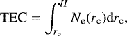
Using the above principle, cometary ionospheric electron density Ne was estimated along the Rosetta trajectories around comet 67P. For this long-term study, we utilized the average Ne over a time window of 320 s when the number of density measurements extracted from the RPC-MIP spectra exceeds 50% of the total number of available spectra during that time window. During an approximately two-year-long period Rosetta monitored in situ the cometary plasma environment from a varying distance between 0 and ~1500 km. Vigren & Galand (2013) predict an Ne altitude profile with a peak ionospheric density above the comet surface. From the analysis of the near-surface cometary ionospheric density measurements during the final descent of Rosetta spacecraft to 67P, a peak in Ne was identified and was found to be located at ~5 km from the cometary nucleus center (Heritier et al. 2017). This result therefore confirmed the previous theoretical expectations of the cometary ionosphere peak density location. This location was shown to be dependent only on the geometry of the nucleus, and to be independent of solar or other external conditions. Using these results, and the fact that Ne follows an  dependence (Edberg et al. 2015), where rc is the cometocentric distance, above the altitude of the peak density (Heritier et al. 2017), we schematically present the rc -dependent ionospheric Ne profile of 67P in Fig. 1. Based on this simple schematic consideration, we define a cometary TEC or the altitude-integrated electron number density as follows:
 (1)
(1)
![\[ \text{where } N_{\textrm{e}}(r_{\textrm{c}}) = \begin{cases} N_{\textrm{p}}\frac{r_{\textrm{p}}}{r_{\textrm{c}}} &\text{for } H \geq r_{\textrm{c}} > r_{\textrm{p}}\\ N_{\textrm{p}}\frac{r_{\textrm{c}} - r_{\textrm{o}}}{r_{\textrm{p}} - r_{\textrm{o}}} &\text{for } r_{\textrm{o}} < r_{\textrm{c}} \leq r_{\textrm{p}}. \end{cases} \]](/articles/aa/full_html/2020/03/aa37022-19/aa37022-19-eq4.png)
In equation (1), ro is the average radius of comet 67P, typically taken as 2 km. The quantity Np represents the peak plasma density and rp is corresponding cometocentric distance which is considered to be 5 km. For practical reasons, we take the upper limit of integration H as 500 km. This ensuresconvergence and is justified by the fact that the cometary plasma density is shown to follow a much steeper variation, closer to  , at larger distances (see Behar et al. 2018) associated with the cometary ion pick-up process in the incoming magnetized solar wind flow; this results in insignificant contribution to cometary ionospheric TEC at large cometocentric distances. It should be noted that this TEC estimation is based on an assumption of radially expanding plasma. However, a radial expansion at the constant velocity of plasma may not be expected out to several 100 km, particularly at a low activity period. During such conditions, density contributions from distances above 100 km may be significantly low. This is discussed later in the paper.
Using the above relations, TEC is finally expressed as a function of Ne and rc :
![\[ \textrm{TEC} = \begin{cases} 4.9\times10^5r_{\textrm{c}}N_{\textrm{e}} &\text{for } 500~\textrm{km} \geq r_{\textrm{c}} > 5~\textrm{km}\\ \frac{73.6}{r_{\textrm{c}} - 2}\times10^5N_{\textrm{e}} &\text{for } 2~\textrm{km} < r_{\textrm{c}} \leq 5~\textrm{km}, \end{cases} \]](/articles/aa/full_html/2020/03/aa37022-19/aa37022-19-eq6.png)
where Ne and rc are obtained from Rosetta measurements in cm−3 and km, respectively, and TEC is obtained in cm−2.
The TEC represents the total number of free thermal electrons contained in a column of unit cross-section along a vertical propagation path from the comet surface to an altitude of 500 km. Because it is an altitude-integrated parameter, TEC is supposed to give a description of the cometary ionosphere that is independent of the Rosetta cometocentric distance rc at the time of measurement. Therefore TEC is more suitable than a single-point Ne value to study the global structure of the cometary ionosphere. For example, TEC can give more complete idea about the altitude extent of the cometary diamagnetic cavity void of magnetic fields (e.g., Goetz et al. 2016a,b; Nemeth et al. 2016; Timar et al. 2017), about the global impacts of space weather events like coronal mass ejections (CMEs; e.g., Witasse et al. 2017; Goetz et al. 2019), corotating interaction regions (CIRs) between solar wind high-speed streams, and slow streams (e.g., Edberg et al. 2016; Hajra et al. 2018b) on the cometary atmosphere.
The main neutral species present in the 67P coma are reported to be H2O, CO2, and CO (Hässig et al. 2015; Le Roy et al. 2015; Fougere et al. 2016). Their ionization threshold wavelengths are ~98, 90, and 89 nm, respectively, below which absorption of solar photons can lead to ionization (e.g., Galand et al. 2016). Thus the solar flux dependence of the cometary plasma can be studied by considering the solar extreme ultraviolet (EUV) radiations. As there was no EUV solar flux monitor on board the Rosetta spacecraft, we used the daily average spectral solar fluxes obtained from the Thermosphere Ionosphere Mesophere Energetics and Dynamics–Solar EUV Experiment (TIMED–SEE; Woods et al. 2005). The fluxes are corrected for the 67P orbit by considering the Earth-Sun-67P angle and an interplanetary solar rotation period of 26 days (Withers & Mendillo 2005). Since the solar flux is proportional to the inverse square of distance from the Sun, the actual fluxes (EUVc) incident on the comet nucleus are estimated by taking into account the heliocentric distance of comet 67P (once the shift in angle has been considered).
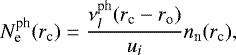
According to analytical ionospheric modeling at the comet (Galand et al. 2016; Vigren et al. 2016), cometary plasma density  at a cometocentric distance rc due to photo-ionization of cometary neutral species l by solar ionizing fluxes is estimated as follows:
 (2)
(2)
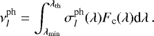
In the above equations,  is the photo-ionization frequency of cometary outgassing neutral species l, ui is the ion bulk velocity, nn (rc) is the cometary neutral density at rc,
  is the total photo-ionization cross-section of the neutral species l having ionization threshold and minimum wavelengths λth and λmin, respectively, and Fc(λ) is the un-attenuated solar ionizing flux at the comet ionosphere. We estimated the photo-ionization frequency, electron density Ne along the Rosetta trajectory, and TEC due to photo-ionization using the above relationships. The TIMED–SEE spectral solar flux extrapolated as described above are used to estimate
  , following Heritier et al. (2018). We considered photo-ionization cross-sections separately for dominating species H2O given in Vigren & Galand (2013) and species CO2 given in Cui et al. (2011). This same procedure was used by Galand et al. (2016) and Heritier et al. (2018) for modeling 67P in situ ionospheric plasma, although the above-mentioned authors also included electron-impact ionization. The λmin is taken as 0.1 nm. Accounting for the range of neutral outflow velocity, we estimated a range of Ne and TEC for ui of 500 m s−1 and 900 m s−1 (Gulkis et al. 2015; Lee et al. 2015; Galand et al. 2016; Hansen et al. 2016; Marshall et al. 2017). The cometary neutral density nn measured by the Rosetta Orbiter Spectrometer for Ion and Neutral Analysis/COmet Pressure Sensor (ROSINA/COPS; Balsiger et al. 2007) was used for the present analysis. It may be mentioned that the ROSINA/COPS nn measurement is sensitive to the neutral composition (Gasc et al. 2017). However, in our model calculation, we took care of this factor in theestimation of photo-ionization frequencies of the species (see Galand et al. 2016).
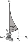 |
Fig. 1 Schematic Ne profile of comet 67P as a function of cometocentric distance rc. The quantity Np represents the peak plasma density and rp is the corresponding cometocentric distance. |
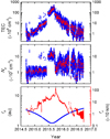 |
Fig. 2 Ionosphere of comet 67P during the Rosetta mission. From top to bottom panels: ionospheric TEC derived from RPC-MIP, observed electron density (Ne) along the Rosetta spacecraft trajectory, and heliocentric distance (rh) of comet 67P (blue, scale on the left), and cometocentric distance (rc) of Rosetta from 67P (red, scale on the right), respectively. Top two panels: the blue points show 320 s average data and red shows the corresponding daily averages (see Sect. 2). |
3 Results
3.1 Cometary TEC variation during the entire Rosetta mission: an overview
The variations of estimated TEC and in situ electron density Ne along the spacecraft trajectory, along with the cometocentric distance rc and the heliocentric distance rh of comet 67P for the entire mission operation interval are shown in Fig. 2. The blue data points in the top two panels correspond to 320 s average RPC-MIP measurements with >50% detection ratio (see Sect. 2), while the red points correspond to their “daily averages”. It should be noted that the comet exhibits roughly two rotations per 24 h period, thus the daily average is performed over roughly two cometary rotations. We also excluded the intervals with prominent solar and interplanetary disturbances (Edberg et al. 2016; Hajra et al. 2018a; Goetz et al. 2019) to study the “quiet-time” ionospheric behavior. The day with cometary brightness outburst was also excluded (Hajra et al. 2017). From Fig. 2 discontinuities can be recorded in Ne and TEC during June 2015. It may be noted that there was a change in Rosetta operation mode on 2015 June 29; LDL was mostly used before and SDL mostly used after. The maximum density retrieved in LDL mode is ~350 cm−3, while plasma density below ~500 cm−3 cannot be measured in SDL mode. However, all RPC-MIP spectra were manually scrutinized to avoid the errors associated with this mode change.
During the entire Rosetta mission operation period, a maximum TEC of ~555 × 109 cm−2 was estimated on 2015 September 7 at a heliocentric distance of ~1.28 au. However, plasma density variations below ~10% would not be detected because of the finite frequency resolution in the RPC-MIP operational mode used to retrieve the plasma density. This may introduce errors in the lowest TEC values as TEC is a linear function of in situ plasma density.
For statistical analysis and comparison, the entire Rosetta observation period is divided into five intervals according to the heliocentric distance and orbital position of comet 67P. These consist of perihelion, where rh < 1.5 au; medium heliocentric distances of 1.5 au < rh < 2 au before and after perihelion; and large heliocentric distances rh > 2.5 au before and after perihelion. The intervals are shown in Table 1. The corresponding seasonal information taken from Heritier et al. (2018) is also shown. The statistical characteristics of TEC during these intervals are summarized in Table 2. The TEC exhibits large variability as evident from significant standard deviations. As 67P approached the Sun, TEC increased and reached its maximum following perihelion, after which it decreased with increasing heliocentric distance. Average diurnal TEC during perihelion is ~(133 ± 84) × 109 cm−2, that is, significantly larger than ~(1–3) × 109 cm−2 recorded at large heliocentric distances (>2.5 au).
Classification of the mission period according to the heliocentric distance rh of comet 67P.
Statistical mean and standard deviations of diurnal mean and median TEC during various orbital phases of comet 67P.
3.2 Cometary TEC dependence on heliocentric distance
The variation of TEC as a function of heliocentric distance rh of 67P is shown in Fig. 3. The green circles in the top panel show all TEC values during the entire mission (320 s average), while blue and red triangles show the daily average TEC during pre- and post- perihelion periods, respectively. The middle and bottom panels show data separately for northern and southern hemispheres, respectively. A clear decrease in TEC with increasing rh can be noted during both pre- and post- perihelion periods. The blue and red lines (top panel) represent the regression equations obtained from regression analysis between logarithm of TEC and rh during pre- and post- perihelion periods, respectively. From this analysis, TEC can be expressed as an exponential function of rh : TEC = Aexp(-Brh), where A and B are constants. The values of the constants and the corresponding correlation coefficients (cc) are given in Table 3. High values of cc confirm significant association of TEC with rh. However, at the same rh, TEC values during the post-perihelion period are significantly (roughly two to four times) larger compared to the pre-perihelion TEC values.This “ionospheric hysteresis effect” is more prominent at large heliocentric distances. This result is also consistent with results shown in Table 2.
Figure 3 (middle and bottom panels) shows clear hemispheric dependence of the hysteresis effect. In the northern hemisphere, pre- and post- perihelion TEC values are quite comparable at all heliocentric distances. However, in the southern hemisphere, post-perihelion TECs are significantly larger than the pre-perihelion values. A more detailed study on the hemispheric asymmetry is presented in Sect. 3.3.
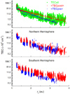 |
Fig. 3 Variation of TEC with heliocentric distance rh. Top panel: the green circles show the 320 s average TEC values during the entire mission operation period, while blue and red triangles show the daily average TEC during pre- and post- perihelion periods, respectively (see Sect. 2). The linear fits between logarithm of TEC and rh are also shown. Middle and bottom panels: pre- (blue) and post- (red) perihelion TEC values in northern and southern hemispheres, respectively. |
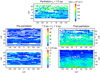 |
Fig. 4 Quiet time average TEC maps during different phases of the Rosetta mission. The color bar maximum values in the top, middle, and bottom panels are different. |
Cometary TEC (in 109 cm−2) vs. heliocentric distance rh (in au) during pre- and post- perihelion periods.
3.3 Hemispheric asymmetry of cometary TEC
Previous studies (e.g., Edberg et al. 2016; Galand et al. 2016; Hajra et al. 2018a) reported that cometary Ne variation exhibits dependences on the cometary sub-spacecraft latitude (λ) and longitude (θ). To verify any λ–θ dependence of TEC, we developed average quiet time TEC maps for the five intervals shown in Table 1. The maps are shown in Fig. 4. The average TEC values at each λ–θ grid are shown in the associated color scales.
In general, the average TEC values decrease with increasing heliocentric distance before and after perihelion. The TEC is larger in thepost-perihelion periods compared to the pre-perihelion intervals for the same heliocentric distance range. These are consistent with the results depicted in Fig. 3 and Table 2. In addition to these, variation in the hemispheric asymmetry is shown in Fig. 4.
During post-perihelion, at both 1.5 au < rh < 2 au and at rh > 2.5 au, TEC values are prominently larger in the southern hemisphere (~(50–70) × 109 cm−2 and ~(6–10) × 109 cm−2, respectively) compared to the northern hemisphere (~(20–30) × 109 cm−2 and ~(2–3) × 109 cm−2, respectively). Thus, on the average, TEC in the southern hemisphere is approximiately three times larger than the TEC in the northern hemisphere during the post-perihelion period. During perihelion, TEC estimations are available from ~70° N latitude to ~60° S latitude of the comet. Around the low- to mid- latitude zone (~20–50°), TEC values of ~(150–200) × 109 cm−2 are recorded in the southern hemisphere, while TEC varies around ~(350–400) × 109 cm−2 in the northern hemisphere. Thus, during perihelion, TEC in the northern hemisphere is approximately two times larger than the southern hemispheric TEC on the average. This clearly shows a reversal of hemispheric asymmetry between perihelion with higher TEC in the northern hemisphere, and post-perihelion with higher TEC in the southern hemisphere. However, such hemispheric asymmetry seems to be less prominent during the pre-perihelion intervals when overall TEC values were smaller.
3.4 Cometary TEC dependence on solar ionizing fluxes
Figure 5 shows the variation of diurnal median TEC with the ionizing EUV fluxes incident on the comet 67P ionosphere (EUVc) at different phases of the cometary activity (Table 1). The TEC is found to increase linearly with increasing EUVc. The correlation coefficient cc of linear regression between TEC and EUVc exhibits an interesting dependence on the heliocentric distance rh. Both during pre- and post-perihelion periods, cc increases with decreasing heliocentric distance. The best correlation is however recorded at distances 1.5 au < rh < 2 au and decreases at larger heliocentric distances rh > 2.5 au. The relationships are statistically significant at the 99.9% confidence level (Student’s t-test; Student 1908).
Considering the contributions of solar ionizing fluxes on the cometary plasma, TEC values due to photo-ionization are estimated for the entire mission. These are compared with the estimated values (red) from the RPC-MIP observations in Fig. 6. The blue and green points in the top two panels correspond to model values computed using ion bulk velocities of 500 and 900 m s−1, respectively.In the top panel, TEC model values are estimated by only considering photo-ionization of H2O, while TEC model estimations in the second panel from top correspond to CO2 as the only ionized neutral species. It is interesting to note that estimated electron density due to photo-ionization of CO2 is larger than that due to photo-ionization of H2O by ~20–40%. This is consistent with results shown by Galand et al. (2016). According to their model study for a pre-perihelion period when comet 67P was at a heliocentric distance of ~3 au, the photo-ionization frequency increased by 18% at most from a pure H2O to a half CO2 and half H2O mixture (Läuter et al. 2018).
The diurnal average TEC values and standard deviations obtained from the actual observations are shown by red points and error bars, respectively, in the top two panels of Fig. 6. For 1.5 au < rh < 2 au, the model values are found to match well with the observed values both during pre- and post-perihelion periods. This result is consistent with the highest correlation coefficients between TEC and solar ionizing fluxes recorded during these periods as shown in Fig. 5. At larger heliocentric distances rh > 2.5 au, modeled values due to photo-ionization are found to underestimate the actual observation. This indicates possible domination of another ionization process over the photo-ionization. On the other hand, the model overestimates the observations during perihelion. This result is in good agreement with the recent study by Vigren et al. (2019), who demonstrate that the standard simplified ionospheric models (e.g., Galand et al. 2016; Heritier et al. 2018) overestimate observed electron density near perihelion, while the level of agreement improves at larger heliocentric distances.
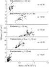 |
Fig. 5 Variation of diurnal median TEC with EUVc. The linear regression fits and regression coefficients (cc) are shown in each plot. All the correlation coefficients are significant at the 99.9% confidence level. |
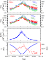 |
Fig. 6 Comparison between observed and modeled TEC at comet 67P during the entire Rosetta mission operation period. In the top two panels, the red points show the diurnally averaged TEC values obtained from actual observation,while the blue and green points correspond to the model TEC values for ion bulk speeds of 500 and 900 m s−1, respectively. Top panel: the modeled TEC values correspond to a pure H2O coma, while they correspond to a pure CO2 coma in thesecond panel from the top. Third panel from the top: corrected EUV fluxes incident on the comet. Bottom panel: variations of rh (blue, legend on the left) and rc (red, legend on the right). |
3.5 Dawn–dusk effects on cometary TEC
The Rosetta spacecraft orbited comet 67P in its terminator plane corresponding to dawn and/or dusk local times. To study the dawn–dusk effects on the cometary TEC, if any, we considered TEC variations during the last four months of the mission, from 2016 June to September, when the comet was between ~3.1 and ~3.8 au from the Sun. All TEC measurements during this period were separated according to local dawn (0400–0800 LT at the sub-spacecraft point) and dusk (1600–2000 LT) time sectors. These are shown in Fig. 7. Dusk TEC values are often larger compared to the dawn-time values. When northern and southern hemispheric values are separated, a clear hemispheric dependence can be noted in the dawn-dusk TEC variability. Overall TEC values are smaller in northern hemisphere compared to those in the southern hemisphere, which is consistent with results shown in previous sections. While dawn and dusk TEC values are comparable (~1.5 × 109 cm−2) in the northern hemisphere, dusk-time TEC values (~10.9 × 109 cm−2) are often significantly larger than the dawn-time TEC values (~3.2 × 109 cm−2) in the southern hemisphere.
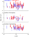 |
Fig. 7 Variation of TEC with heliocentric distance rh during 2016 June–September. The blue empty and red filled circles correspond to TEC values during dawn (0400–0800 LT) and dusk (1600–2000 LT) local times, respectively. While the top panel shows the data for both hemispheres combined, the middle and bottom panels show TEC values in northern and southern hemispheres, respectively. |
4 Discussion
4.1 TEC variability
We explored cometary ionospheric variability during solar/ interplanetary quiet intervals. The TEC values depict high variability of the quiet-time ionosphere of comet 67P. During the entire Rosetta mission, comet 67P exhibited a large TEC variation by ~2 orders of magnitude on average, with a daily-average peak of ~(133 ± 84) × 109 cm−2 near perihelion. This may be compared to a neutral outgassing rate variation by ~3 orders of magnitude when the heliocentric distance varied from ~1.2 to 3.8 au (Hansen et al. 2016; Heritier et al. 2018). The present study suggests an exponential decay of TEC with the heliocentric distance. This can be related to a steep evolution of the neutral outgassing rate with heliocentric distance, typically between  to
to  as reported in previous studies (e.g., Snodgrass et al. 2013; Simon Wedlund et al. 2016; Biver et al. 2019).
There were very few previous attempts to estimate cometary TEC based on remote sensing and/or flyby experiments. Edenhofer et al. (1985) suggested a peak TEC value of ~10 × 1012 cm−2 of comet 1P/Halley (at a heliocentric distance of ~0.9 au) based on a Doppler simulation during Giotto spacecraft encounter on 1986 March 14. The ionospheric sounding of the comet by coherent dual frequency (C-band: 5.8 GHz and L-band: 0.9 GHz) radio waves during the Vega-1 spacecraft flyby on 1986 March 6 revealed a peak cometary TEC of ~5 × 1012 cm−2 (Pätzold et al. 1997). Both of these studies used radial distribution of cometary electron density to estimate TEC as is done in the present work. The Halley TEC values are ~2 orders of magnitude larger than the peak TEC value at comet 67P obtained in the present work. This is consistent with the fact that the cometary neutral outgassing rate of 67P is significantly less (by ~2 orders of magnitude) than that at comet Halley (see, e.g., Mandt et al. 2016; Ksanfomality 2017, and references therein). Compared to comet 67P TEC, the highly variable terrestrial ionospheric TEC is ~3 orders of magnitude larger near dayside maximum (see Browne et al. 1956; Evans 1956; Hargreaves 1992; Mannucci et al. 1998; Tsurutani et al. 2004; Chakraborty & Hajra 2008; Hajra 2012; Hajra et al. 2016, and references therein).
4.2 TEC hysteresis
A cometary ionospheric hysteresis effect is revealed for the first time in the present work. At the same heliocentric distance, overall TEC values are larger during post-perihelion than during pre-perihelion intervals. When separated in hemispheres, the hysteresis is found to be a dominant feature over the southern hemisphere, while north hemispheric TEC values are found to be comparable between pre- and post-perihelion intervals. It may be noted that Hansen et al. (2016) report local outgassing rate peak ~20 days after perihelion, attributed to some plausible hemispheric effects and neutral density variation (see Hansen et al. 2016; Heritier et al. 2018). While the neutral outgassing rate shows asymmetry pre- and post-perihelion, TEC hysteresis may not be solely related to the cometary neutral density asymmetry. This is supported by the present work showing lower ionizing solar fluxes incident on the comet ionosphere after perihelion compared to the pre-perihelion fluxes (Fig. 6), confirming earlier results (Heritier et al. 2018). This latter result is related to the fact that the entire mission interval was in the descending part of the solar activity cycle 24. An additional cause may be that the inbound equinox was much closer to perihelion compared to the outbound equinox.
The asymmetry may also be triggered by an asymmetry in electron-impact ionization, which is a key ionizing source at large heliocentric distances (Heritier et al. 2018). Other important factors contributing to TEC variability may be the attenuation of solar ionizing fluxes by the cometary neutrals and dissociative recombination between electrons and ions (Heritier et al. 2018; Beth et al. 2019). Both these processes can act to reduce TEC values. However, along the Rosetta trajectory the impacts of the dissociative recombination and solar absorption were found to be insignificant before and after perihelion (Heritier et al. 2018). Heritier et al. (2018) show that solar flux attenuation or photo-absorption effect may only be significant near the surface of the comet, while the dissociative recombination effect is significant at larger cometocentric distances. As TEC is an altitude-integrated plasma parameter, TEC variability is supposed to be modulated by both these processes.
As mentioned above, the photo-ionization contribution was lower during post-perihelion. Thus higher observed TEC values during this period may be related to larger electron-impact ionization rates during post-perihelion.
With the decrease of solar activity owing to the descending phase of solar cycle, the photo-ionization frequency gets smaller, while the electron-impact ionization frequency remains about constant or may even increase during post-perihelion phase. This raises the question of why there would be more electron-impact ionization and whether the electron acceleration processes could be more efficient during post-perihelion, and in such a case, why. Further study is required to fully understand this behavior.
4.3 TEC hemispheric asymmetry
We developed average latitude-longitude maps of TEC during different cometary activity conditions (heliocentric distances). In general, while pre-perihelion TEC exhibits approximate hemispheric homogeneity on average, significant asymmetry was recorded during perihelion and post-perihelion orbital periods of comet 67P. The maps can be compared with outgassing H2O maps developed by Hansen et al. (2016). Based on both observation and modeling, the H2O production rate was shown to be larger in the northern hemisphere compared to the southern hemisphere during pre-perihelion. This was shown to reverse during and after perihelion. Very asymmetric electron-impact ionization frequency is considered to have compensated the lower neutral density in the southern hemisphere exhibiting winter season during pre-perihelion (see Galand et al. 2016). On the other hand, during post-perihelion, the electron-impact asymmetry could not compensate for larger neutral density over the southern hemisphere exhibiting summer season (Heritier et al. 2018).
During perihelion, average TEC values were roughly two times larger in the northern hemisphere that was exhibiting autumn season compared to that in the southern hemisphere where it was spring. However, the neutral outgassing rate was reported to be higher in the southern hemisphere than in the northern hemisphere (Hansen et al. 2016; Biver et al. 2019). The anti-correlation between TEC and neutral outgassing rate hemispheric variations deserves further study. Engelhardt et al. (2018) report an overall larger population of cold (<0.1 eV) electrons in the southern hemisphere during perihelion. This may suggest less electron-impact ionization in the southern hemisphere compared to the northern hemisphere. This is consistent with observed hemispheric asymmetry in TEC during perihelion. However, near perihelion, electron-impact ionization is reported to be a negligible source of ionization (Heritier et al. 2018).
During post-perihelion, the hemispheric asymmetry was reversed and stronger; the southern hemisphere exhibited approximately three times larger TEC values compared to the northern hemisphere. This result is correlated with hemispheric inhomogeneity of outgassing rate reported by Gasc et al. (2017). Strengthening of the asymmetry (compared to that during perihelion) may be related to additional effects of electron-impact ionization during post-perihelion. However, this has yet to be confirmed quantitatively.
The hemispheric asymmetry is also reflected in the local dawn-dusk TEC variability during the last four months of the mission (>3 au). In the southern hemisphere, dusk time TECs were significantly higher than the dawn time TEC values. No such dawn-dusk asymmetry was prominent in the northern hemisphere, where the overall TEC values are lower than in the southern hemisphere. As there is no significant difference in ionizing solar fluxes between dawn and dusk, the dawn-dusk asymmetry should be directly associated with higher neutral outgassing at dusk because of surface thermal inertia. However, this requires further confirmation.
4.4 TEC dependence on photo-ionization
To quantify the photo-ionization contribution to the TEC variability, we estimated the expected TEC values due to photo-ionization of cometary neutrals throughout the Rosetta mission. This process “detrends” the TEC variability with respect to the variability in the neutral outgassing rate. While photo-ionization seems to be the dominating contributor around 1.5 au < rh < 2 au, it underestimates the actual observations at large heliocentric distances (rh > 2.5 au). The latter result corroborates the finding of Heritier et al. (2018) that electron-impact ionization is a dominating source of ionization at large heliocentric distances. Around perihelion (rh < 1.5 au), modeled TEC due to photo-ionization seems to overestimate the actual observations of TEC. This is probably related to the overestimation of solar ionizing fluxes near perihelion and an underestimation of loss processes. Ionizing solar fluxes are suggested to suffer from absorption by cometary neutrals (Rees 1989; Beth et al. 2019), although at the location of Rosetta the electron density may not be affected by it (Beth et al. 2019). Solar flux also suffers from scattering and absorption by cometary dust (Johansson et al. 2017) and loss due to dissociative recombination (Heritier et al. 2018) around perihelion. This may result in reduction of actual ionospheric density (TEC) around perihelion.
In addition, the model discrepancy may be associated with the possibility that the bulk speed of the plasma may be higher than that of the neutrals or that the plasma are decoupled from the neutrals. In fact, Odelstad et al. (2018) report ion speeds markedly higher than the neutral outgassing velocity. Acceleration along an ambipolar electric field and inefficient coupling to the neutrals could cause such a situation (Vigren & Eriksson 2017, 2019; Vigren et al. 2019).
5 Summary and conclusions
We have used the in situ cometary plasma measurements by the Rosetta spacecraft to assess and interpret the variability of the cometary ionospheric TEC of comet 67P over the whole comet escort phase for the first time. Because it is an altitude-integrated plasma parameter, TEC gives a more comprehensive description of the cometary ionosphere compared to plasma measurements along the spacecraft trajectory. The present study covers the entire Rosetta mission operation period of approximately two years in order to explore the cometary ionospheric evolution depending on varying heliocentric distances. The main findings of the present work may be summarized as follows:
- 1.
Cometary TEC exhibits large variability with diurnally averaged peak value of ~(133 ± 84) × 109 cm−2 reached during perihelion (rh < 1.5 au). It decreases exponentially with heliocentric distance attaining values ~2 orders of magnitude lower at larger heliocentric distance (rh > 2.5 au).
- 2.
A clear ionospheric hysteresis effect is observed in heliospheric variation of TEC. At similar heliocentric distances of the comet, TEC values are significantly (roughly two to four times) larger during post-perihelion compared to pre-perihelion TEC values. The hysteresis effect is more prominent in the southern hemisphere of the comet and at larger heliocentric distances. Our study suggests possible contributions of larger electron-impact ionization (production) during post-perihelion and, to an lesser extent, of larger dissociative recombination (loss) effects during pre-perihelion.
- 3.
On average, significant hemispheric asymmetry is recorded in TEC during perihelion and post-perihelion periods, while the asymmetry was less pronounced during pre-perihelion periods. During perihelion (rh < 1.5 au), the northern hemisphere exhibited roughly two times larger TEC values compared to the southern hemisphere. The asymmetry reversed and became stronger during post-perihelion when average TEC in the southern hemisphere was approximiately three times larger than that in the northern hemisphere. Variation in relative importance of electron-impact ionization and photo-ionization processes (seasonal variation of outgassing rates) are suggested as the plausible reasons.
- 4.
A hemispheric asymmetry was also observed in dawn-dusk variations of TEC. While dawn and dusk TEC values are comparable in the northern hemisphere, dusk-time TEC values are more than three times larger than the dawn-time TEC values in the southern hemisphere.
- 5.
While TEC is found to increase with increasing solar ionizing fluxes incident on the comet ionosphere at any heliocentric distance, the strongest association was noted just after perihelion (1.5 au < rh < 2 au).
- 6.
We estimated the expected TEC values due to photo-ionization of cometary neutrals by solar ionizing fluxes. At moderate heliocentric distances (1.5 au < rh < 2 au), photo-ionization contribution matches well with the actual TEC observations. At larger heliocentric distances (rh > 2.5 au), photo-ionization contribution underestimates the actual observations implying importance of electron-impact ionization process in the cometary ionosphere, as reported previously (Galand et al. 2016; Heritier et al. 2018).
In this paper, we presented a method to estimate the altitude-integrated electron number density (TEC) from the comet 67P surface to an arbitrarily chosen altitude of 500 km, beyond which the cometary plasma density is supposed to decrease significantly. While TEC can be a suitable parameter to study the behavior of a cometary ionosphere which is expanding radially, care is suggested to be taken in the interpretation during varying cometary and solar activity conditions. For example, at low activity a radial expansion at constant velocity of the plasma may not be expected out to several 100 km. However, from the presented results in this work, TEC revealed a clearer picture of the cometary ionosphere compared to in situ spacecraft plasma measurement, in terms of ionospheric hysteresis effect, hemispheric asymmetry, and solar activity dependence. Further study can be done on solar wind coupling of cometary ionosphere using this parameter.
Acknowledgements
Rosetta is an European Space Agency (ESA) mission with contributions from its member states and National Aeronautics and Space Administration (NASA). The work of R.H. is financially supported by the Science & Engineering Research Board (SERB), a statutory body of the Department of Science & Technology (DST), Government of India through Ramanujan Fellowship. The work at LPC2E/CNRS was supported by CNES, ESEP, and by ANR under the financial agreement ANR-15-CE31-0009-01. Work at Imperial College London is supported by STFC of UK under grant ST/N000692/1 and ESA under contract No.4000119035/16/ES/JD. Portions of the research were conducted at the Jet Propulsion Laboratory, California Institute of Technology, under contract with NASA. M.R. is supported by the State of Bern and the Swiss National Science Foundation (SNSF, 200020_182418). The work of Z.N. was supported by the János Bolyai Research Scolarship of the Hungarian Academy of Sciences. This work has made use of AMDA and RPC quick-look database to provide an initial overview of the event studied. This is provided through a collaboration between theCentre de Données de la Physique des Plasmas (CDPP) (supported by CNRS, CNES, Observatoire de Paris, and Université Paul-Sabatier, Toulouse) and Imperial College London (supported by the UK Science and Technology Facilities Council). The data used in this paper are available on the ESA Planetary Science Archive (PSA).
References
- Balsiger, H., Altwegg, K., Bochsler, P., et al. 2007, Space Sci. Rev., 128, 745 [NASA ADS] [CrossRef] [Google Scholar]
- Behar, E., Tabone, B., Saillenfest, M., et al. 2018, A&A, 620, A35 [Google Scholar]
- Beth, A., Galand, M., & Heritier, K. L. 2019, A&A, 630, A47 [NASA ADS] [CrossRef] [EDP Sciences] [Google Scholar]
- Biver, N., Bockelée-Morvan, D., Hofstadter, M., et al. 2019, A&A, 630, A19 [NASA ADS] [CrossRef] [EDP Sciences] [Google Scholar]
- Broiles, T. W., Burch, J. L., Chae, K., et al. 2016, MNRAS, 462, S312 [CrossRef] [Google Scholar]
- Browne, I. C., Evans, J. V., Hargreaves, J. K., & Murray, W. A. S. 1956, Proc. Phys. Soc., 69, 901 [NASA ADS] [CrossRef] [Google Scholar]
- Carr, C., Cupido, E., Lee, C. G. Y., et al. 2007, Space Sci. Rev., 128, 629 [NASA ADS] [CrossRef] [Google Scholar]
- Chakraborty, S. K., & Hajra, R. 2008, Ann. Geophys., 26, 47 [Google Scholar]
- Churyumov, K. I., & Gerasimenko, S. I. 1972, IAU Symp., 45, 27 [NASA ADS] [Google Scholar]
- Clark, G., Broiles, T. W., Burch, J. L., et al. 2015, A&A, 583, A24 [NASA ADS] [CrossRef] [EDP Sciences] [Google Scholar]
- Cravens, T. E., Kozyra, J. U., Nagy, A. F., Gombosi, T. I., & Kurtz, M. 1987, J. Geophys. Res., 92, 7341 [Google Scholar]
- Cui, J., Galand, M., Coates, A. J., Zhang, T. L., & Müller-Wodarg, I. C. F. 2011, J. Geophys. Res., 116, A04321 [NASA ADS] [Google Scholar]
- Edberg, N. J. T., Eriksson, A. I., Odelstad, E., et al. 2015, Geophys. Res. Lett., 42, 4263 [CrossRef] [Google Scholar]
- Edberg, N. J. T., Eriksson, A. I., Odelstad, E., et al. 2016, J. Geophys. Res. Space Phys., 121, 949 [NASA ADS] [CrossRef] [Google Scholar]
- Edenhofer, P., Bird, M. K., Volland, H., Esposito, P. B., & Porsche, H. 1985, Adv. Space Res., 5, 201 [NASA ADS] [CrossRef] [Google Scholar]
- Engelhardt, I. A. D., Eriksson, A. I., Stenberg Wieser, G., et al. 2018, MNRAS, 477, 1296 [Google Scholar]
- Eriksson, A. I., Boström, R., Gill, R., et al. 2007, Space Sci. Rev., 128, 729 [NASA ADS] [CrossRef] [Google Scholar]
- Eriksson, A. I., Engelhardt, I. A. D., André, M., et al. 2017, A&A, 605, A15 [NASA ADS] [EDP Sciences] [Google Scholar]
- Evans, J. V. 1956, Proc. Phys. Soc., 69, 953 [NASA ADS] [CrossRef] [EDP Sciences] [Google Scholar]
- Fougere, N., Altwegg, K., Berthelier, J.-J., et al. 2016, MNRAS, 462, S156 [CrossRef] [Google Scholar]
- Fuselier, S. A., Altwegg, K., Balsiger, H., et al. 2015, A&A, 583, A2 [NASA ADS] [CrossRef] [EDP Sciences] [Google Scholar]
- Fuselier, S. A., Altwegg, K., Balsiger, H., et al. 2016, MNRAS, 462, S67 [NASA ADS] [CrossRef] [EDP Sciences] [Google Scholar]
- Galand, M., Héritier, K. L., Odelstad, E., et al. 2016, MNRAS, 462, S331 [CrossRef] [Google Scholar]
- Gasc, S., Altwegg, K., Balsiger, H., et al. 2017, MNRAS, 469, S108 [Google Scholar]
- Gilet, N., Henri, P., Wattieaux, G., Cilibrasi, M., & Béghin, C. 2017, Radio Sci., 52, 1432 [NASA ADS] [CrossRef] [Google Scholar]
- Glassmeier, K.-H., Boehnhardt, H., Koschny, D., Kührt, E., & Richter, I. 2007, Space Sci. Rev., 128, 1 [NASA ADS] [CrossRef] [Google Scholar]
- Goetz, C., Koenders, C., Hansen, K. C., et al. 2016a, MNRAS, 462, S459 [Google Scholar]
- Goetz, C., Koenders, C., Richter, I., et al. 2016b, A&A, 588, A24 [Google Scholar]
- Goetz, C., Tsurutani, B. T., Henri, P., et al. 2019, A&A, 630, A38 [NASA ADS] [CrossRef] [EDP Sciences] [Google Scholar]
- Goldstein, R., Burch, J. L., Mokashi, P., et al. 2017, MNRAS, 469, S262 [Google Scholar]
- Gulkis, S., Allen, M., von Allmen, P., et al. 2015, Science, 347, 0709 [Google Scholar]
- Hajra, R. 2012, PhD Thesis, University of Calcutta, Kolkata, West Bengal, India [Google Scholar]
- Hajra, R., Chakraborty, S. K., Tsurutani, B. T., et al. 2016, J. Space Weather Space Clim., 6, A29 [Google Scholar]
- Hajra, R., Henri, P., Vallières, X., et al. 2017, A&A, 607, A34 [NASA ADS] [CrossRef] [EDP Sciences] [Google Scholar]
- Hajra, R., Henri, P., Myllys, M., et al. 2018a, MNRAS, 480, 4544 [Google Scholar]
- Hajra, R., Henri, P., Vallières, X., et al. 2018b, MNRAS, 475, 4140 [NASA ADS] [CrossRef] [Google Scholar]
- Hansen, K. C., Altwegg, K., Berthelier, J.-J., et al. 2016, MNRAS, 462, S491 [Google Scholar]
- Hargreaves, J. K. 1992, The Solar-Terrestrial Environment: an Introduction to Geospace - the Science of the Terrestrial Upper Atmosphere, Ionosphere, and Magnetosphere, Cambridge Atmospheric and Space Science Series (Cambridge: Cambridge University Press) [Google Scholar]
- Hässig, M., Altwegg, K., Balsiger, H., et al. 2015, Science, 347, 0276 [CrossRef] [Google Scholar]
- Henri, P., Vallières, X., Hajra, R., et al. 2017, MNRAS, 469, S372 [Google Scholar]
- Heritier, K. L., Henri, P., Vallières, X., et al. 2017, MNRAS, 469, S118 [CrossRef] [Google Scholar]
- Heritier, K. L., Galand, M., Henri, P., et al. 2018, A&A, 618, A77 [NASA ADS] [CrossRef] [EDP Sciences] [Google Scholar]
- Johansson, F. L., Odelstad, E., Paulsson, J. J. P., et al. 2017, MNRAS, 469, S626 [NASA ADS] [CrossRef] [Google Scholar]
- Ksanfomality, L. V. 2017, Physics-Uspekhi, 60, 290 [Google Scholar]
- Läuter, M., Kramer, T., Rubin, M., & Altwegg, K. 2018, MNRAS, 483, 852 [NASA ADS] [Google Scholar]
- Lee, S., von Allmen, P., Allen, M., et al. 2015, A&A, 583, A5 [NASA ADS] [CrossRef] [EDP Sciences] [Google Scholar]
- Le Roy, L., Altwegg, K., Balsiger, H., et al. 2015, A&A, 583, A1 [NASA ADS] [CrossRef] [EDP Sciences] [Google Scholar]
- Mandt, K. E., Eriksson, A., Edberg, N. J. T., et al. 2016, MNRAS, 462, S9 [Google Scholar]
- Mannucci, A. J., Wilson, B. D., Yuan, D. N., et al. 1998, Radio Sci., 33, 565 [NASA ADS] [CrossRef] [Google Scholar]
- Marshall, D. W., Hartogh, P., Rezac, L., et al. 2017, A&A, 603, A87 [NASA ADS] [CrossRef] [EDP Sciences] [Google Scholar]
- Myllys, M., Henri, P., Galand, M., et al. 2019, A&A, 630, A42 [NASA ADS] [CrossRef] [EDP Sciences] [Google Scholar]
- Nemeth, Z., Burch, J., Goetz, C., et al. 2016, MNRAS, 462, S415 [Google Scholar]
- Nilsson, H., Stenberg Wieser, G., Behar, E., et al. 2015, Science, 347, 0571 [NASA ADS] [CrossRef] [Google Scholar]
- Odelstad, E., Eriksson, A. I., Johansson, F. L., et al. 2018, J. Geophys. Res., 123, 5870 [NASA ADS] [CrossRef] [Google Scholar]
- Pätzold, M., Neubauer, F. M., Andreev, V. E., & Gavrik, A. L. 1997, J. Geophys. Res., 102, 2213 [NASA ADS] [CrossRef] [Google Scholar]
- Rees, M. H. 1989, Physics and Chemistry of Upper Atmosphere (Cambridge: Cambridge University Press) [Google Scholar]
- Simon Wedlund, C., Kallio, E., Alho, M., et al. 2016, MNRAS, 587, A154 [Google Scholar]
- Snodgrass, C., Tubiana, C., Bramich, D. M., et al. 2013, A&A, 557, A33 [NASA ADS] [CrossRef] [EDP Sciences] [Google Scholar]
- Student. 1908, Biometrika, 6, 1 [CrossRef] [Google Scholar]
- Timar, A., Nemeth, Z., Szego, K., et al. 2017, MNRAS, 469, S723 [Google Scholar]
- Trotignon, J. G., Michau, J. L., Lagoutte, D., et al. 2007, Space Sci. Rev., 128, 713 [NASA ADS] [CrossRef] [Google Scholar]
- Tsurutani, B., Mannucci, A., Iijima, B., et al. 2004, J. Geophys. Res., 109, A08302 [NASA ADS] [CrossRef] [Google Scholar]
- Vigren, E., & Eriksson, A. I. 2017, AJ, 153, 150 [NASA ADS] [CrossRef] [Google Scholar]
- Vigren, E., & Eriksson, A. I. 2019, MNRAS, 482, 1937 [NASA ADS] [CrossRef] [Google Scholar]
- Vigren, E., & Galand, M. 2013, ApJ, 772, 33 [Google Scholar]
- Vigren, E., Altwegg, K., Edberg, N. J. T., et al. 2016, AJ, 152, 59 [NASA ADS] [CrossRef] [Google Scholar]
- Vigren, E., Edberg, N. J. T., Eriksson, A. I., et al. 2019, ApJ, 881, 6 [Google Scholar]
- Wattieaux, G., Gilet, N., Henri, P., Vallières, X., & Bucciantini, L. 2019, A&A, 630, A41 [NASA ADS] [CrossRef] [EDP Sciences] [Google Scholar]
- Witasse, O., Sánchez-Cano, B., Mays, M. L., et al. 2017, J. Geophys. Res., 122, 7865 [Google Scholar]
- Withers, P., & Mendillo, M. 2005, Planet. Space Sci., 53, 1401 [NASA ADS] [CrossRef] [Google Scholar]
- Woods, T. N., Eparvier, F. G., Bailey, S. M., et al. 2005, J. Geophys. Res., 110, A01312 [NASA ADS] [CrossRef] [Google Scholar]
All Tables
Classification of the mission period according to the heliocentric distance rh of comet 67P.
Statistical mean and standard deviations of diurnal mean and median TEC during various orbital phases of comet 67P.
Cometary TEC (in 109 cm−2) vs. heliocentric distance rh (in au) during pre- and post- perihelion periods.
All Figures
|
Fig. 1 Schematic Ne profile of comet 67P as a function of cometocentric distance rc. The quantity Np represents the peak plasma density and rp is the corresponding cometocentric distance. |
| In the text | |
|
Fig. 2 Ionosphere of comet 67P during the Rosetta mission. From top to bottom panels: ionospheric TEC derived from RPC-MIP, observed electron density (Ne) along the Rosetta spacecraft trajectory, and heliocentric distance (rh) of comet 67P (blue, scale on the left), and cometocentric distance (rc) of Rosetta from 67P (red, scale on the right), respectively. Top two panels: the blue points show 320 s average data and red shows the corresponding daily averages (see Sect. 2). |
| In the text | |
|
Fig. 3 Variation of TEC with heliocentric distance rh. Top panel: the green circles show the 320 s average TEC values during the entire mission operation period, while blue and red triangles show the daily average TEC during pre- and post- perihelion periods, respectively (see Sect. 2). The linear fits between logarithm of TEC and rh are also shown. Middle and bottom panels: pre- (blue) and post- (red) perihelion TEC values in northern and southern hemispheres, respectively. |
| In the text | |
|
Fig. 4 Quiet time average TEC maps during different phases of the Rosetta mission. The color bar maximum values in the top, middle, and bottom panels are different. |
| In the text | |
|
Fig. 5 Variation of diurnal median TEC with EUVc. The linear regression fits and regression coefficients (cc) are shown in each plot. All the correlation coefficients are significant at the 99.9% confidence level. |
| In the text | |
|
Fig. 6 Comparison between observed and modeled TEC at comet 67P during the entire Rosetta mission operation period. In the top two panels, the red points show the diurnally averaged TEC values obtained from actual observation,while the blue and green points correspond to the model TEC values for ion bulk speeds of 500 and 900 m s−1, respectively. Top panel: the modeled TEC values correspond to a pure H2O coma, while they correspond to a pure CO2 coma in thesecond panel from the top. Third panel from the top: corrected EUV fluxes incident on the comet. Bottom panel: variations of rh (blue, legend on the left) and rc (red, legend on the right). |
| In the text | |
|
Fig. 7 Variation of TEC with heliocentric distance rh during 2016 June–September. The blue empty and red filled circles correspond to TEC values during dawn (0400–0800 LT) and dusk (1600–2000 LT) local times, respectively. While the top panel shows the data for both hemispheres combined, the middle and bottom panels show TEC values in northern and southern hemispheres, respectively. |
| In the text | |
Current usage metrics show cumulative count of Article Views (full-text article views including HTML views, PDF and ePub downloads, according to the available data) and Abstracts Views on Vision4Press platform.
Data correspond to usage on the plateform after 2015. The current usage metrics is available 48-96 hours after online publication and is updated daily on week days.
Initial download of the metrics may take a while.