| Issue |
A&A
Volume 633, January 2020
|
|
|---|---|---|
| Article Number | A3 | |
| Number of page(s) | 13 | |
| Section | Interstellar and circumstellar matter | |
| DOI | https://doi.org/10.1051/0004-6361/201936820 | |
| Published online | 19 December 2019 | |
Late encounter events as source of disks and spiral structures
Forming second generation disks
Zentrum für Astronomie der Universität Heidelberg, Institut für Theoretische Astrophysik,
Albert-Ueberle-Str. 2,
69120
Heidelberg,
Germany
e-mail: This email address is being protected from spambots. You need JavaScript enabled to view it.
Received:
1
October
2019
Accepted:
9
November
2019
Abstract
Context. Observations of arc-like structures and luminosity bursts of stars >1 Myr in age indicate that at least some stars undergo late infall events.
Aims. We investigate scenarios of replenishing the mass reservoir around a star via capturing and infalling events of cloudlets.
Methods. We carried out a total of 24 three-dimensional hydrodynamical simulations of cloudlet encounters with a Herbig star of mass 2.5 M⊙ using the moving-mesh code AREPO. To account for the two possibilities of a star or a cloudlet traveling through the interstellar medium (ISM), we put either the star or the cloudlet at rest with respect to the background gas.
Results. For absent cooling in the adiabatic runs, almost none of the cloudlet gas is captured as a result of high thermal pressure. However, second-generation disks easily form when accounting for cooling of the gas. The disk radii range from several 100 to ~1000 au and associated arc-like structures up to 104 au in length form around the star for runs with and without stellar irradiation. Consistent with angular momentum conservation, the arcs and disks are larger for larger impact parameters. Accounting for turbulence in the cloudlet only mildly changes the model outcome. In the case of the star being at rest with the background gas, the disk formation and mass replenishment process is more pronounced and the associated arc-shaped streamers are longer lived.
Conclusions. The results of our models confirm that late encounter events lead to the formation of transitional disks associated with arc-shaped structures such as observed for AB Aurigae or HD 100546. In addition, we find that second-generation disks and their associated filamentary arms are longer lived (>105 yr) in infall events, when the star is at rest with the background gas.
Key words: hydrodynamics / protoplanetary disks / planetary systems / accretion, accretion disks / stars: kinematics and dynamics / circumstellar matter
International Postdoctoral Fellow of Independent Research Fund Denmark (IRFD).
© ESO 2019
1 Introduction
Stars form and evolve in the dynamically evolving medium of giant molecular clouds (GMC; Blitz 1993) as a consequence of gravitational collapse of so-called prestellar cores; these prestellar cores emerge as a result of existing turbulence in the GMC (Padoan & Nordlund 2002; Mac Low & Klessen 2004). Protostars grow in mass as long as they are sufficiently fed with mass from the circumstellar envelope of gas and dust (Larson 1969). Models based on the assumption of a collapsing spherical prestellar core in isolation show that this phase typically lasts for ~100 kyr (e.g., Machida et al. 2010; Masson et al. 2016). During this initial time interval, a disk forms around the protostar (e.g., Machida & Matsumoto 2011; Li et al. 2011; Seifried et al. 2013; Tomida et al. 2015; Wurster et al. 2018). These disks are the birthplaces of planets (Keppler et al. 2018) and therefore commonly referred to as protoplanetary disks. Their lifetimes range between ~1 Myr and several Myr (Haisch et al. 2001; Mamajek 2009) before they dissipate. However, the formation process of stars is heterogeneous depending on the environment in which the protostar is embedded (Kuffmeier et al. 2017, 2018). Previous models already demonstrated the possibility of late accretion events around protostars (Baraffe et al. 2009; Vorobyov & Basu 2010; Padoan et al. 2014) as a possible explanation of the observed spread in protostellar luminosities (Kenyon et al. 1990; Evans et al. 2009; Dunham et al. 2010). Gaseous condensations of size ~100 au with masses ≪1M⊙ referred to as cloudlets have been observed previously (Langer et al. 1995; Heiles 1997; Falgarone et al. 2004).
Apart from that, late accretion may not only directly affect the properties of the accreting star (Kunitomo et al. 2017; Jensen & Haugbølle 2018), but also the properties of surroundings of the star (Jørgensen et al. 2015; Frimann et al. 2017), and in particular its protoplanetary disk. The possibility of accretion onto star-disk systems has been studied in previous works (Moeckel & Throop 2009; Wijnen et al. 2016, 2017a,b). Against the background of planet formation and the existence of disks, replenishing the mass reservoir of disks via late accretion is one possible solution to the “missing mass problem” in planet formation theory (Mulders et al. 2015; Kuffmeier et al. 2017; Nixon et al. 2018; Manara et al. 2018). The possibility of late mass accrual after dispersal of the primordial disk also raises the following question: If new material can fall onto a star hundreds of thousand of years after its formation, would it be possible to form a new disk again? Dullemond et al. (2019; hereafter referred to as D19) considered the scenario in which a star that is traveling through the interstellar medium (ISM) captures gas from a condensation of gas in the GMC after the priomordial disk has already dissipated. The scenario, referred to as “cloudlet capture”, is related to the Bondi–Hoyle–Lyttleton (hereafter BHL) process (Hoyle & Lyttleton 1939; Bondi & Hoyle 1944; Bondi 1952). Cloudlet capture differs from BHL accretion in the sense that the BHL process considers direct accretion onto the star, while in the cloudlet scenario we investigate the effect of angular momentum of the cloudlet on the morphology of the gas around the moving star. In particular, we are interested in whether cloudlet capture events can lead to the formation of a new generation of disks and/or to the formation of arcs and streamers, such as observed for AB Aurigae (Nakajima & Golimowski 1995; Grady et al. 1999; Fukagawa et al. 2004), FU Ori, Z CMa or V1057Cyg (Liu et al. 2016, 2018).
Apart from the scenario of cloudlet capture, in which the star travels through the ISM and potentially captures gas from its surrounding, we can also consider a similar scenario of a cloudlet that actively moves toward a star at rest with its surrounding. We refer to this scenario as the infall scenario. While being mostly equal by virtue of Galilean invariance, the difference between the two scenarios is the velocity of the low-density space-filling background medium in which both the star and the cloudlet are embedded. In this paper, we consider the scenarios of cloudlet capture and infalling cloudlets. We carry out a total of 24 models in a parameter study with the moving-mesh code AREPO1 (Springel 2010; Pakmor et al. 2016) to investigate the consequences of captured and infalling cloudlets at a stage after a star has already formed in its parental GMC.
We structure the paper as follows: in Sect. 2, we present the different model setups. In Sect. 3, we present the results of our parameter study. In particular, we present results from models with increasing complexity by first considering the setup of D19 as a default and consistently varying the setup by adding turbulence, removing the background velocity, and accounting for stellar irradiation. We compare our results with observed structures and also discuss the limitations of our model in Sect. 4. In Sect. 5, we then summarize our main results and provide the main conclusions.
2 Methods
We based our three-dimensional models of cloudlets being captured by a star on the simulations presented in D19, which modeled the interaction via the PLUTO code2 (Mignone et al. 2007). However, for this work we simulated the encounter using the moving-mesh hydrodynamics code AREPO. This code solves the Euler equations using a finite-volume approach on an unstructured Voronoi mesh that moves with the flow. As explained by Goicovic et al. (2019) in the context of stars that are disrupted by supermassive black holes, AREPO is well suited for this kind of problems because of its quasi-Lagrangian nature, which retains the high accuracy of mesh-based techniques, while not imposing any preferred grid orientation. Additionally, the fluxes are computed in the reference frame of themesh faces, which greatly reduces advection errors, and does not lose accuracy with increasing gas velocity. Finally, the full spacial and temporal adaptivity of AREPO allowed us to refine or derefine cells as desired, similar to adaptive mesh refinement codes. In the case of our models, this allowed us to maintain constant mass resolution in the cloudlet, while keeping a minimum spatial resolution in the low-density regions of the ambient medium.
Based on the description by Klessen & Hennebelle (2010), we used as in D19 the following equation for the cloudlet mass
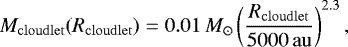 (1)
(1)
such that the mass solely depends on the radius of the cloudlet Rcloudlet. The star is modeled as an external Newtonian potential, which is located at the center of the domain with an initial mass of 2.5 M⊙. In order to avoid divergent accelerations, this gravitational potential has a softening radius of 5 au around the center. Furthermore, since this scale is significantly smaller than the typical size of the gas cells, in the vicinity of the star we imposed an additional refinement criterion to those already mentioned to maintain a certain number of gas cells per softening length (see Appendix B). Finally, to mimic the capture of gas by the star and to reduce the computational cost of these models, we implemented accretion onto the central potential. Within 25 au of the center, all gas cells are drained of 90% of their mass at each timestep and directly added to the central mass. While the star is at rest, the cloudlet and the surrounding gas has an initial bulk velocity of v = (v∞, 0, 0), where v∞ is set to 105 cm s−1.
We modeled the cloudlet capture in a large box with periodic boundary conditions. The box length is defined as Lbox = 148 Rcloudlet. We stopped the simulations early enough such that the results are unaffected by the assumption of periodic boundary conditions. Altogether, we conducted a series of 24 models as summarized in Table 1. The basic setups are the same as considered in D19 for instantaneous cooling (isothermal cases I1, I2, I3) and without cooling (adiabatic cases A1, A2, A3). In other words, we used a ratio of specific heat of  in the adiabatic case, and γ = 1 for the isothermal runs. In the adiabatic runs, we inserted the center of the cloud at (x, y, z) = (−7.82 Rcloudlet, −b, 0), where b is the impact parameter. We set the background temperature to Tbg = 8000 K inspired by the temperature of a warm neutral medium (Field et al. 1969). The cloudlet temperature of the adiabatic runs is Tcloudlet = 30 K, and the background density is
 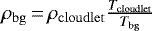 . This choice guarantees that the cloudlet is pressure confined in the adiabatic runs.
For the isothermal runs we set the temperature to T = Tcloudlet = Tbg = 10 K everywhere in the domain, and we set the background density to 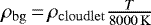 . As the cloudlet is not pressure confined in the isothermal run, it immediately starts to expand. To nevertheless model the capturing and infalling process, we placed the cloudlet initially closer to the central potential at a location of (x, y, z) = (−3.22 Rcloudlet, −b, 0).
Additionally, we carried out a set of models in which we added turbulence to the initial cloud setups. These runs are labeled with an additional “_t”. The turbulent velocity of each gas cell is drawn from Gaussian random distribution using the prescription described in Dubinski et al. (1995). We sampled the velocities in Fourier space with a a power spectrum of |vk|2 ∝ k−4, where k is the wavenumber of the perturbation, and the power index is chosen to match the velocity dispersion observed in molecular clouds (Larson 1981). Finally, the velocity field is normalized such that the internal velocity dispersion of the cloudlet is 10% of its initial bulk speed, i.e., we multiplied each velocity by
 (2)
(2)
where σv is the velocity dispersion of field before normalization. We note that, with this choice of parameters, the internal turbulence is supersonic with typical Mach numbers around 4.
The models presented up to this point consider the scenario in which the star travels through the medium at a given speed and captures mass from its surroundings, but we are also interested in the related scenario of infall. In this case, only the individual gas condensation has a relative velocity difference compared to the star co-moving with the background velocity. We modeled this scenario by only giving a velocity of v = (v∞, 0, 0) to the cloudlet, while setting the background gas and the central mass potential at rest. The infall models are labeled with an additional _nw to indicate that the background gas is at rest (“no wind” of the background gas).
Furthermore,to model the presence of the star beyond its gravitational influence more adequately, it is important to consider that stellar irradiation heats up the surrounding gas. To mimic this effect, we adopted a radial temperature profile that considers the irradiation of a perfect blackbody, constant in time, as follows:
 (3)
(3)
where L* is the luminosity of the star, σSB is the Stefan-Boltzmann constant, and r is the radial distance from the star, i.e., the center of our domain. Applying this recipe, the temperature is 10 K at radial distances of r > 776 au from the star. We refer to the runs accounting for stellar irradiation with Irr, and we investigate the effect of this heating implementation using the setups of the isothermal runs.
Additionally, using the stellar irradiation recipe, we carried out three runs with varying impact parameter b, which we label by appending the value of b in au, namely 0, 500 and 1000. Except for b, the initial size and location of the cloudlet is identical to the setup of IrrI1_t.
The cloudlet is initially resolved with a total of 106 cells and we smoothly decreased the resolution beyond the cloudlet to a lower background resolution as illustrated in Fig. A.1. Starting with this smooth transition in the initial setup prevents spurious shock waves from being launched at the edge of the cloud immediately after starting the simulations. We ran all models without self-gravity, hence the central mass is the only source of gravity.
Summary of the setups of the different runs.
3 Results
We first give a qualitative description of the sequence of cloudlet capturing and infall for the adiabatic and isothermal setups. In the following, we show results from runs in which we account for stellar irradiation; we then quantify the encounter events by focusing on the amount of captured mass and on the properties of forming disks.
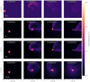 |
Fig. 1 Illustration of the column density in the planes perpendicular to the orientation of the angular momentum vector for the setups of the adiabatic run A1 (upper panels) and the isothermal run I1 (lower panels) at times (t0 = 0, t1 = 4 tdyn, t2 = 8 tdyn, and t3 = 16 tdyn. |
3.1 Sequence for the adiabatic and isothermal setups
In this subsection, we qualitatively present the process of encounter events using the thermodynamical description used in D19. In Fig. 1, we illustrate column densities in the plane perpendicular to the angular momentum vector around the central star for the cases of A1_t, I1, I1_t and I1_t_nw at time t = 0, 12, 24, 36 tdyn, where  and Rcloudlet is the cloudlet radius and v∞ is the escape velocity, which we set to 1 km s−1 = 105 cm s−1. The projected area is 16 000 au × 16 000 au. The plots illustrate that gas is affected by the central mass in all setups. The process differs significantly between the adiabatic and isothermal models. In the adiabatic run, the gas from the cloudlet initially engulfs the star in a halo-like manner and then forms a transient arc-like structure (as seen in the second panel). However, most of the gas passes by the star in a hyperbolic orbit due to its intrinsic angular momentum and disperses during the further evolution, such that almost no gas is captured in the adiabatic scenario (third and fourth panel).
In the isothermal runs, we also see the formation of bent structures, but rather as tails associated with the formation of disks than as remnants of dispersing halos. In contrast to the adiabatic scenario, mass is captured in the isothermal run and disks of radii r ≫ 100 au easily form. The details of the process differ between the setups, but in general gas passes by in the adiabatic runs, while it can remain in the vicinity of the star and lead to the formation of disks in the isothermal runs.
This behavior is expected considering that the isothermal and adiabatic setups are two extreme scenarios of either perfect or absent cooling. In the adiabatic run, thermal pressure increases when the gas gets compressed during the capturing phase. Therefore, the fresh gas leads to the formation of an intermittent envelope, but not to the formation of a disk. In the isothermal run, infalling gas remains cold, and disks quickly form owing to conservation of angular momentum. Our results for the models without turbulence are in good agreement with the results based on simulations with PLUTO presented in D19.
As seenin the third row of Fig. 1, the sequence is qualitatively the same regardless of whether we start with or without an initially turbulent cloudlet. The infall scenarios (_nw runs), in which only the cloudlet is moving and the background gas is at rest, are similar during the early evolutionary phase, but differ at later times. Comparing the morphology of the arc-like structures, we find that in the capturing scenario of a traveling star, the bent arms are dragged by the motion of the background gas, leading to morphological differences of the arm structures around the star (see fourth column in Fig. 1). In general, the disk shrinks in radius over time and more mass is swept away by the background velocity for the capturing scenarios (I1 and I1_t). In the infall scenario, mass remains in the vicinity of the star for a longer time correlating with longer lasting disks.
3.2 Toward more realistic modeling: accounting for stellar irradiation
In the models presented above, we consider two extreme scenarios of perfect or absent cooling. In reality, dense gas in the ISM is cold, but the central star acts as a radiation source heating up its surrounding. We account for the effect of stellar irradiation by adopting the radially dependent temperature profile that is constant in time given by Eq. (3). For the luminosity of the star, we assume L* = 50 L⊙, similar to the luminosity of AB Aurigae where L = 47 L⊙ (Tannirkulam et al. 2008). We run these models for an initially turbulent cloudlet and with background velocity. Similar to the isothermal models, we find the formation of large disks after the encounter phase of the cloudlet with the star. As illustrated in the projection plots along the three different coordinate axes in Fig. 2, the results are only mildly different from the pure isothermal runs. This is not surprising considering the large radial extent of the disks far beyond r = 100 au and considering that stellar irradiation only mildly increases the temperature of the initially cold gas (T = 10 K) at large radii (e.g., T(100 au) ≈ 74 K, T(1000 au) ≈ 23.5 K). Although this temperature profile is still rather simplified, the models nevertheless demonstrate the possibility of newly forming disks for cloudlet encounters for already formed stars when accounting for stellar irradiation. We contend that we overestimate rather than underestimate heating by the central star because we neglect any shielding by the gas. Moreover, the column density profiles in the left panels of Fig. 2 illustrate the formation of large arc-structures extending to distances beyond several 103 au from the star associated with second generation disks of several 100 au to r ~ 1000 au in size.
3.3 Varying the impact parameter b
As seen in D19 and confirmed in this work, the capturing process varies for various initial cloud parameters Rcloudlet and impact parameter b. To better constrain the effect of the impact parameter b, we varied b for otherwise identical conditions as in IrrI1_t (runs IrrI1_t0, IrrI1_t500, and IrrI1_t1000). Analogous to Fig. 1, we illustrate the evolution by showing snapshots at t = 0, 12, 24, 36 tdyn of the runs IrrI1_t0, IrrI1_t500, IrrI1_t1000, and IrrI1_t in Fig. 3. In the case of b = 0, i.e., zero net angular momentum of the cloudlet, we see that the cloudlet passes the central mass and gets disrupted without leaving any trace of forming adisk. Applying a non-zero impact parameter leads to the formation of disks with larger and longer lasting disks for increasing impact parameters, as expected from angular momentum conservation. Moreover, in the cases of larger impact parameters b = 1000 au and b = 1774 au, associated with the formation of disks, we find the formation of arcs that are several 1000 au in length.
Although the amount of enclosed mass and the properties of the disks quantitatively differ for the runs with different initial cloudlet sizes or impact parameters, the sequences are generally similar. Given a non-zero impact parameter, disks and bent arm structures form for models with cooling of the gas (isothermal and stellar irradiation runs), while disk formation is suppressed in the adiabatic runs.
3.4 Captured mass
To quantify the capturing process more, we show the evolution of mass that is enclosed within 1000 au from the central star (upper panels) as well as the amount of accreted mass (lower panels) over 39 dynamical times tdyn for the different runs with the setups of A1 and I1 (left panels) and A2 and I2 (right panels) in Fig. 4. We compute the amount of accreted as the cumulative sum of the difference of total mass in the simulation between the different snapshots. In both the adiabatic and isothermal setups, we can see a characteristic early peak in enclosed mass that is almost independent of whether the model is run with or without turbulence or background velocity. The peak occurs earlier in the isothermal setups as a consequence of initially placing the cloudlet closer to the star to prevent cloudlet dispersal before the encounter. For the smaller cloudlet radius (upper left panel), a higher percentage of cloudlet mass reenters the region around the star within 1000 au after the initial fly-by, whereas relatively more cloudlet mass is swept away with the background velocity instead of being captured for the larger cloudlet radius (upper right panel). For the setup with the largest cloudlet radius (I3 setups, not shown), the peak is almost entirely absent.
In a comparison of the runs with identical impact parameter b and cloudlet radius Rcloudlet, the evolution differs significantly after the encounter of the cloudlet with the star. The plots demonstrate the fundamental difference of absent capturing in the adiabatic case and mass growth in the isothermal case. While in the isothermal runs a substantial amount of mass is kept within a radial distance of 1000 au from the central star, the enclosed mass rapidly decreases again after the early peak during the encounter in the adiabatic run. In the adiabatic cases, the mass only marginally grows to about ~ 10−2 Mcloudlet with respect to the initial setup.
For the isothermal setups we find that the amount of enclosed mass decreases after the early peak, too. However, the amount of enclosed mass decays less after the initial peak than in the adiabatic runs. In sharp contrast to the adiabatic runs, the amount of captured mass increases again after the early enhancement. Especially, for relatively small cloudlet sizes (I1, I2), we find significant mass growth at later evolutionary stages for the isothermal setups. The smaller the cloudlet radius Rcloudlet, the more mass relative to the mass of the cloudlet is captured again after the peak during the encounter. Our analysis shows that the amount of enclosed mass exceeds the first peak for small enough Rcloudlet. The reason for this is twofold. First, given an identical impact parameter (such as for setups 1 and 2) part of the gas is further away from the star for large cloudlets, and hence this gas is less affected by the gravitational potential of the star. Second, the density of the cloudlet is given by
 (4)
(4)
and using Eq. (1), we obtain a scaling of the density with initial cloudlet radius Rcloudlet as
 (5)
(5)
Recalling that by construction the background density is  shows that both the cloudlet and the background volume density are larger for smaller cloudlet sizes. As a consequence, more mass is available from the background for the models with smaller cloudlet radii, while the cloudlet has lower mass than for models withlarger cloudlet radii. Additionally, smaller cloudlets disperse more quickly for the isothermal setups owing to the higher density, and hence the higher pressure gradient between background gas and cloudlet gas. As seen for the scenarios of I2 and even more for the I1 scenarios in Fig. 4, this can even lead to a state in which the amount of enclosed mass is higher than the initial cloudlet size. The enclosed mass profiles show that for small enough impact parameters part of the cloudlet mass flies by the star and departs from it, but bounces back as a result of the stellar gravitational potential, and hence gas can accrete onto the star in a trajectory as illustrated in the projection plots in Fig. 1.
Concerning the differences among the models with initially identical Rcloudlet and b, we confirm that the amount of captured mass (upper panel in Fig. 4) and accreted mass (lower panel in Fig. 4) is almost identical, regardless whether the models are run with or without turbulence and with or without our recipe of stellar irradiation. Therefore, the results show that the velocity deviations due to turbulence in the cloudlet are of secondary importance for the overall process of mass replenishment around the star. However, during the later evolution we find stronger deviations among the profiles for the runs with background velocity compared to the infall scenario without background velocity. For the runs including the background velocity, we find a second peak in the mass profile, which is absent for the infall scenario without background velocity. For the runs with background velocity, the second enhancements in the mass profiles occur after less dynamical times for higher cloud radii. However, we point out that the concept of a dynamical time based on the initial cloudlet radius loses its meaning at later stages, when the cloudlet is destroyed owing to the combination of dispersal and the earlier encounter event.
In the infall cases, more mass continuously falls toward the central star and replenishes the mass reservoir around the star (upper panel in Fig. 4); subsequently this mass accretes onto the star (lower panel in Fig. 4). As a consequence of the absent background wind that sweeps mass away from the central gravitational potential, the amount of accreted mass is significantly higher for the infall scenario compared to the other scenarios. Compared to the purely isothermal runs, we find a mildly higher amount of enclosed mass, but a lower amount of accreted mass at late times for the runs incorporating our stellar irradiation recipe; see in particular the results for setup 2 in the right panels of Fig. 4. This difference is caused by the additional thermal pressureclose to the star that prevents gas from accreting onto the central potential as directly as in the isothermal runs.
As expected from angular momentum conservation, we confirm that for identical cloudlet size Rcloudlet, the smaller b, the quicker the encountering cloudlet mass accretes onto the central star. This is in line with the presence of larger disk and arc structures as described in the comparison of impact parameter b (see Fig. 3). In the case of smaller b, a higher amount of mass is quickly “lost” to the central star, and hence cannot lead to the formation of substantial secondary disks or arcs. In general, our results show that encounters with a cloudlet can efficiently enrich the mass reservoir around the star regardless of the details of the specific setups.
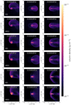 |
Fig. 2 Illustration of the column density in the three planes of the coordinate system (left panels: xy, middle panels: yz, right panels: xz) for the setups of the isothermal runs after 10 dynamical times (t = 10 tdyn). Panels in odd rows correspond to pure isothermal runs and panels in even rows correspond to the cases with stellar irradiation. |
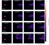 |
Fig. 3 Column density in the planes perpendicular to the orientation of the angular momentum vector for runs IrrI1_t0, IrrI1_t500, IrrI1_t1000, and IrrI1_t at times (t0 = 0, t1 = 4 tdyn, t2 = 8 tdyn, and t3 = 16 tdyn. |
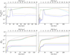 |
Fig. 4 Evolution of captured mass and accreted mass for altogether 14 runs.Upper panels: amount of mass within 1000 au from the central potential. Lower panels: corresponding amount of accreted mass. The line style and color is used consistently for the upper and lower plots. Left panels: A1 (blue solid), A1_t (green dashed), A1_t_nw (red dotted), I1 (cyan solid), I1_t (purple dashed), I1_t_nw (black dotted), and IrrI1_t (yellow solid); right panels: A2 (blue solid), A2_t (green dashed), A2_t_nw (red dotted), I2 (cyan solid), I2_t (purple dashed), I2_t_nw (black dotted), and IrrI2_t (yellow solid). |
3.5 Second generation disk formation
3.5.1 Velocity profile
As illustrated in the exemplary projection plots in Figs. 1, 2, and 3, disks form for the isothermal runs with and without stellar irradiation. To better constrain the properties of the velocity field, we computed the average velocity in a total of 30 shells with logarithmically increasing radius ri from 1 to 104 au around the star. The height of each bin is set to h = ±0.1 ri and the orientation is such that the radial direction is perpendicular to the orientation of the total angular momentum vector computed for the gas located within 1000 au from the star. In Fig. 5, we show the velocity profile at t = 16 tdyn for the differentmodels (without turbulence, with turbulence, and infall with turbulence) of A1, I1, A2, I2, A3, and I3. The plot demonstrates that the velocity profiles of the disks in the isothermal and stellar irradiation runs are in good agreement with the profile of a Keplerian disks, while the adiabatic runs typically do not show any signs of Keplerian rotation (except for a mild signature in the A3 run). The velocity profiles show that the isothermal disks typically extend to radii of ≈ 500 to ≈ 1000 au.
A comparison of the isothermal models (without turbulence, with turbulence, and with turbulence and background velocity) shows that the models only slightly deviate for radii smaller than r ≲ 1000 au. As shown above, the most significant differences occur between the infall scenario without background velocity compared to the scenarios with background velocities. As a consequence of enhanced accretion onto the central sink, the azimuthal velocities in the infall runs of I1 and I2 are lower than for the runs with background velocity for r ≲ 1000 au. Beyond that radius the velocity falls off more sharply in the runs with background velocity than in the runs without background velocity. This tendency can be seen more clearly for the runs with larger cloudlet radii (I2 in the middle panel and I3 in the right panel). The more shallow decay of the rotational velocity profile is induced by the fact that the background starts spiraling toward the central star, while in the other runs the velocity profiles of the lower density gas significantly deviate from Keplerian as a consequence of the intrinsic background flow. Regardless of the subtle differences among the different setups, the results of our isothermal and stellar irradiation runs show that the disks are indeed rotationally supported and relatively large as expected from angular momentum conservation.
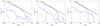 |
Fig. 5 Velocity profiles at t = 16 tdyn for the different runs. Left panel: A1 (blue solid), A1_t (green dashed), A1_t_nw (red dotted), I1 (cyan solid), I1_t (purple dashed), I1_t_nw (black dotted), and IrrI1_t (yellow solid); middle panel: A2 (blue solid), A2_t (green dashed), A2_t_nw (red dotted), I2 (cyan solid), I2_t (purple dashed), I2_t_nw (black dotted), and IrrI2_t (yellow solid); right panel: A3 (blue solid), A3_t (green dashed), A3_t_nw (red dotted), I3 (cyan solid), I3_t (purple dashed), I3_t_nw (black dotted), and IrrI3_t (yellow solid). The black solid line corresponds to the Keplerian velocity
|

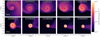 |
Fig. 6 Column density in the planes perpendicular to the orientation of the angular momentum vector for run IrrI1_t at different times. Upper panel, from left to right: t1 = 4 tdyn, t2 = 8 tdyn, t3 = 12 tdyn, t4 = 16, t5 = 20 tdyn, and lower panel, from left to right: t6 = 24 tdyn, t7 = 28 tdyn, t8 = 32 tdyn, t9 = 36 tdyn and at the end of the simulation t10 = 39 tdyn. |
3.5.2 Column density profile
Rather thancarry out a detailed study of the properties of the corresponding disks, the scope of this paper is to investigate the overall possibility of whether mass replenishment induced by cloudlet encounters leads to the formation of bent structures and second-generation disks. However, the distribution of mass in the disk is a crucial parameter when speculating about planet formation ina second-generation disk. Therefore, we analyze the evolution of the disks in our IrrI1_t in more detail. To illustrate the sequence of disk formation and evolution more clearly, we show projection plots in the plane of the disk for a region of 3200 × 3200 au at ten different times in Fig. 6. Furthermore, we show the azimuthally averaged profiles of the surface density at the corresponding times in Fig. 7 (left panel: 4 tdyn, 8 tdyn, 12 tdyn, 16 tdyn, and 20 tdyn; right panel: 24 tdyn, 28 tdyn, 32 tdyn, 36 tdyn, and 39 tdyn). We use the same radial spacing as for the computation of the velocity profile and the columns extend to the entire size of the domain.
Generally, we find that the surface density profiles undergo a typical sequence. During the encounter, a disk starts to form with maximum density at r ≈ 100 au and connects to the background with a larger spiral arm. During the further evolution, the disk becomes more compact, leading to an increase of Σ ranging between a few 100 to ≈1000 au; there is erosion of the outer part of the disk due to the background velocity. Over time, the bump in Σ decreases again and migrates toward smaller radii (see Fig. 7). Interestingly, a spiral arm structure decoupled from the larger scale environment starts to form in the disk and compacts together with the shrinking disk. The compactification phase leads to an enhancement of density at a radius of a few 100 au with a steep drop inside and outside the evolving bump. That means that consistent with the mass distributions in transitional disks most of the gas is located in the outer part of the disk, although the inner decrease in density is favored by our accretion recipe.
Gas located in the vicinity of the central potential accretes and causes a drop in the surface density profile. Simultaneously, gas with initially large angular momentum contributes to the mass budget of the disk. The outer edge of the disk becomes steeper because the high-density gas initially located in the cloudlet has either already fallen onto the disk or is continuously swept away in the case of a present background wind.
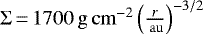
For comparison, in Fig. 7, we also plot the slope of the minimum mass solar nebula (MMSN)  in the azimuthally averaged column density profile. During the early formation of the disk, the column density profile is similar to a power-law function ranging between ~100 and ~1000 au, which is roughly consistent with the slope of the MMSN. However, the radial extent is rather large compared to a primordial disk that forms during the early phase of protostellar collapse, and the power-law description is only transient and appropriate for at most a few 104 kyr.
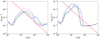 |
Fig. 7 Azimuthally averaged column density in the planes. The column densities are computed perpendicular to the orientation of the angular momentum vector for run IrrI1_t. The profiles correspond to the times represented in the projection plots in Fig. 6. Left panel: t1 = 4 tdyn (blue solid), t2 = 8 tdyn (green dashed), t3 = 12 tdyn (red dotted),t4 = 16 (cyan solid), and t5 = 20 tdyn (purple dashed); right panel: t6 = 24 tdyn (blue solid), t7 = 28 tdyn (green dashed), t8 = 32 tdyn (red dotted),t9 = 36 tdyn (cyan solid), and t10 = 39 tdyn (purple dashed). The red dashed line corresponds to the profile of the MMSN,
|
4 Discussion
In this section, we discuss the limitations of our initial conditions and justify the absence of physical effects such as magnetic fields in our model setup. Moreover, we compare our results with observations of structures around young stellar objects, and we discuss the impact of late encounter events on the formation process of stars, their disks, and eventually planets.
4.1 Initial conditions
To carry out a feasible parameter study consistently, we adopted a rather simplified setup. The initial conditions of our models are idealized such that we adopted a two-phase medium consisting of a perfectly spherical cloudlet and a smooth background medium. As described in the introduction GMCs are threaded by filaments, and hence in reality the GMC is not as smooth as considered in our setup. Nevertheless, gas condensations of higher mass similar to our cloudlets likely exist, although their shape may deviate significantly from a perfect sphere. Considering the star formation process in a GMC, the analysis of Jensen &Haugbølle (2018) shows that some stars undergo late accretion events that cause an increase in luminosity > 1 Myr after their birth. Our scenario is idealized, but observations of luminosity bursts (Kenyon et al. 1990; Evans et al. 2009; Dunham et al. 2010) indicate that late infall, and hence late encounter events, happen for at least some stars. Testing the frequency of such events requires the analysis of star formation simulations, in which the evolution of the stars has evolved with sufficient resolution for a few million years. Along that line, we point out that the main effect of mass replenishment is independent from the shape of the captured or infalling cloudlet as long as the gas encounters the star closely enough. Considering the formation of disks and their associated larger scale arc structures, we also expect to see disk formation as a consequence of angular momentum conservation for realistic elongated gas condensations as long as the impact parameter is small enough that mass can be stripped off.
4.2 Additional physical effects: accretion, irradiation and magnetic fields
Another simplification of our initial condition is the approximation of a star as a point of constant mass. In reality, a young star accretes mass, acts as a strong luminosity source, and affects its surrounding via irradiation. Although, gas can accrete onto the central massif it fulfills the accretion criterion of being gravitationally bound and close enough to the sink, our recipe is very simple compared to more expensive simulations investigating the statistical properties of star formation (e.g., Federrath et al. 2011; Greif et al. 2011; Haugbølle et al. 2018). The recipe leads to a drop of the inner density profile; we tested that, for a larger accretion region of 50 au, the drop of the surface density profile consistently occurs at a larger radii. To get a more accurate profile at smaller distances would be possible using a smaller softening radius and smaller accretion radius. However, as the computational time step scales with the Keplerian speed, the simulation time would become too long for our purposes. Previous models have shown that late infall events correlate with enhanced accretion rates of up to ~ 10−5 M⊙ yr−1 over timescales of Δt ~ 103 yr (Baraffe et al. 2012; Padoan et al. 2014). However, in this study we are interested in the formation of second-generation disks and structures on scales of ~1000 au, rather than in the accretion rate of the already formed host star. Obtaining more realistic accretion rates would require that we run a globalsimulation covering a larger range of scales and incorporating corresponding effects present in the GMC (e.g., Haugbølle et al. 2018; Bate 2018; Wurster et al. 2019). Accretion also enhances the luminosity of the host star due to L ∝Ṁ, and can hence cause radiation. In some of our runs, we account for stellar irradiation as a constant parameter; we also find that replenishment of gas in the stellar surrounding and the formation of second generation disks are at most barely affected by stellar irradiation. Certainly, our temperature relation T(r), which is purely dependent on radius and is constant in time, is very simplified. But given that we assume a rather strong luminosity of 50 L⊙ and no shielding, we rather over- than underestimate irradiation from the central star in our cases. For more realistic setups, we would also need to account for the effects of stellar irradiation from background and neighboring stars, which would affect the thermal pressure in the cloudlet and forming disk.
In our models, we do not account for the presence of magnetic fields in GMCs. Adding magnetic fields to our setup would provide an efficient way of transporting angular momentum from the freshly forming disk via magnetic braking (Mestel & Spitzer 1956). Hence, we expect that magnetic fields would allow the gas to more densely populate the inner parts of the disks (r ≲ 100 au) and also yield smaller disk sizes than seen in our models.
Certainly, constraining these additional effects is important and interesting, but beyond the purpose of this paper. Our aim is to constrain the properties of encounter events rather than to carry out a comprehensive zoom-in simulations of star and disk formation (Kuffmeier et al. 2017, 2018; Bate 2018; Wurster et al. 2019). By carrying out these more simplified case studies, we have the power to vary the key parameters systematically, and hence to understand the underlying processes. Nevertheless, to make further progress in understanding capture and infall events, more advanced models are required that provide better statistics about the probabilities and properties of such encounter events.
4.3 Comparison with observations
The presence of a large bent arm around AB Aurigae is a prominent candidate for the outcome of a late encounter event (Nakajima & Golimowski 1995). Our models show that disks are typically a few to several 100 au in radius and the large-scale arc-like structures typically extend to distances of several 1000 au from the second-generation disk. The combination of a disk size of at least 430 au (Fukagawa et al. 2004), the large arc-shaped reflection nebula ranging from ~1300 to ~6000 au (Grady et al. 1999), and the age of AB Aurigae between 2 Myr (van den Ancker et al. 1998) and 4 Myr (DeWarf et al. 2003) is intriguingly consistent with the results of our scenario. Moreover, our study shows the frequent formation of spiral arms inside second-generation disks, which is consistent with scattered light observations of a spiral arm in the disk around AB Aurigae (Grady et al. 1999; Fukagawa et al. 2004).
Another candidate for a late infall event of a cloudlet is the 10 Myr (van den Ancker et al. 1998) old star HD 1000546 (Grady et al. 2001; Ardila et al. 2007) with a disk up to about 300 au and an arc-shaped envelope extending to about 1000 au from the southwest part of the disk. As discussed in depth in D19, arc-shaped structures seem to be more common around Herbig stars than lower mass stars, which might be a consequence of the higher gravitational potential of Herbig stars corresponding to more pronounced arcs or streamers.
Although AB Aurigae and HD 100546 are the most prominent candidates for an ongoing cloudlet encounter event, other Herbig Ae stars may have undergone encounter events in their past, too. In this context, we want to raise attention to the effect of the background flow on the large-scale arcs. At the end of the simulations (corresponding to about 105 yr) with background velocity, the large-scale arc-shaped structures have been or are about to be swept away by the background gas, while a second-generation disks can still be present. Therefore, some disks around older stars may be the result of a late encounter event and thus a second-generation disk.
Apart from the possibility of encounter events after dispersal of the primordial disk considered in this work, similar encounter events may well happen at earlier stages of the star formation process. For instance, in recent magnetohydrodynamical zoom-in simulations, analogous to Offner et al. (2010), Kuffmeier et al. (2019) find that protostellar companions form with initially wider separation and subsequently approach each other, thereby also replenishing the mass reservoir of the primary stars. Prominent candidates for an encounter event happening at earlier times are FU Orionis and Z CMa. Both sources show the presence of bent arms of several 1000 au in size connected to them (Nakajima & Golimowski 1995; Liu et al. 2016, 2018), and both stars experienced episodic accretion events in the past. Therefore, the concept of infall of fresh gas after the initial protostellar collapse phase already seems to apply at earlier stages.
Considering encounter events at a stage when the primordial disk is still present raises another interesting question. Given that the second-generation disks in our study typically have lower densities at radii less than 100 au, infall of material with different angular momentum might be an alternative explanation for misalignment of inner and outer disks as observed for HD 142527 (Avenhaus et al. 2014; Marino et al. 2015), HD 135344B (Stolker et al. 2016), or HD 100453 (Benisty et al. 2017). In an upcoming paper, we are investigating the effect of infall events similar to that studied in this work, but the infall event we are studying for the future work has a primordial disk.
Moreover, the density distribution in the second-generation disks correlates with a pressure bump at large radii. As a consequence, we expect dust to pile up in the outer part of the disk (Whipple 1972; Brauer et al. 2008), thereby opening a possible path for planet formation at large radii in these second-generation disks if enough mass is provided by a late encounter event.
5 Summary and conclusions
In this paper, we investigate multiple scenarios of a cloudlet flying by a star that has finished its early phase of formation. We carried out a parameter study with the moving-mesh code AREPO consisting of a total of 24 three-dimensional hydrodynamical simulations. In our standard runs, we consider a 2.5 M⊙ star that travels through the ISM and encounters a cloudlet with varying size Rcloudlet and impact parameter b. Building up on these standard runs (capturing scenario), we then consistently analyze the effect of adding turbulence to the initial cloudlet setup; we also consider the scenario in which only the cloudlet is moving toward the star, while the background gas and the star are at rest (infall scenario). All of these runs are carried out for two extreme cases of perfect cooling (isothermal setup) and no cooling (adiabatic run). In the final step, we also investigate a capturing scenario in which we account for stellar irradiation by adopting a radially dependent temperature profile rather than a pure isothermal or adiabatic setup.
Owing to substantial thermal pressure support, we find no or only modest replenishment of gas during an encounter event for the adiabatic runs, which is consistent with previous results. In contrast, for all isothermal runs, we find that a substantial amount of mass is captured by the star at distances of up to ~ 1000 au from the star. These results are in good agreement with previous results by D19 using the PLUTO code. Accounting for stellar irradiation does not hinder capturing of the gas and the additional thermal pressure at most mildly reduces the infall onto the central potential. We therefore conclude that stellar irradiation only affects the capturing process on radial distances of ~10 au or less, but not the overall presence of rotational structures such as arcs and disks. Adding turbulence to the cloudlet only causes very mild deviations.
By following the amount of mass that is enclosed within a radial distance of 1000 au from the star (Menc), we find a characteristic sequence of the encounter event for smaller cloudlet radii and substantial impact parameters b. First, the cloudlet flies by the star, thereby leading to a local maximum in the amount of enclosed mass. Afterward, part of the passing mass returns toward the star from the opposite direction due to the gravitational force of the star. Without background velocity (infall scenario), Menc continuously increases because of infall of the background gas. With background velocity (capturing scenario) Menc decreases after a second local maximum because the background gas is swept away by the background flow, and hence there is not enough infall to compensate for the amount of gas accreting onto the star.
We find that an encounter event quickly leads to the formation of large disks with sizes of several 100 au for runs accounting for cooling, i.e., the isothermal and stellar irradiation runs. The impact parameter b and cloudlet radius Rcloudlet, and hence the angular momentum of the cloudlet, determine both the inner and outer radial extent of the Keplerian profile of the disks. The azimuthal velocity profile tapers off more softly in the infall scenario than in the capturing scenario. In the capturing scenario, the background wind sweeps away the low-density gas, thus leading to a steep drop in the rotational velocity profile beyond the radial extent of the disk (r ~ 100 to 1000 au).
Similar to observations around Herbig stars, we find the presence of arc-like structures extending from the outer parts of the disk to distances of about 104 au. These arc structures are bent and preserved longer in the infall scenario. Consistent with angular momentum conservation, we find that the extent of rotational structures such as spiral arms, arcs, and disks decreases with decreasing impact parameter b. For identical impact parameter b, but larger cloudlet radius Rcloudlet, less mass is captured and accretes onto the star relative to the initial cloudlet mass.
The column density profiles of the disks initially follow a column density distribution that is roughly consistent with a slope of  , and afterward develops toward a profile with a bump at a few ~100 au. Toward the end of the sequence the bump in the column density migrates toward smaller radii (about 100 au) and starts shrinking again. The evolution is correlated with the formation and evolution of a spiral structure that becomes increasingly narrow and dense over time.
Our results show how star-cloudlet encounters can replenish the mass reservoir around an already formed star. Furthermore, the results demonstrate that arc structures observed for AB Aurigae or HD 100546 are a likely consequence of such late encounter events. We find that large second-generation disks can form via encounter events of a star with denser gas condensations in the ISM millions of years after stellar birth as long as the parental GMC has not fully dispersed. The majority of mass in these second-generation disks are located at large radii, which is consistent with observations of transitional disks.
Acknowledgements
The research of M.K. is supported by a research grant of the Independent Research Foundation Denmark (IRFD) (international postdoctoral fellow, project number: 8028-00025B). M.K. acknowledges the support of the DFG Research Unit “Transition Disks” (FOR 2634/1, DU 414/23-1). FGG acknowledges support from DFG Schwerpunktprogramm SPP 1992 “Diversity of Extrasolar Planets” grant DU414/21-1. Last but not least, we thank the referee for his constructive comments and suggestions on an earlier draft of the manuscript.
Appendix A: Initial grid setup
The cells in our simulations consist in the high resolution gas of the cloudlet, together with a low resolution medium. Because the latter fills the whole domain, the size difference between the cells of the cloudlet and the background can be very large. This creates sharp gradients in the contact areas of this two phases, even when we impose pressure equilibrium. To avoid spurious shocks induced by these differences, we initialize our background grid such that the volume difference does not go above a certain threshold. For these models we choose a volume difference of 5.
In practice, we put the cloudlet configuration in a small cubic grid such that the background cells satisfy the volume difference. Then this configuration is surrounded by a slightly larger box under the same condition, and so on until the whole domain is filled with gas. An illustration of the initial setup is shown in Fig A.1.
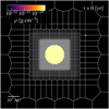 |
Fig. A.1 Slice of the initial setup of the grid. This illustrate our procedure to guarantee a modest transition between the highly resolved cloud (resolution not shown) and the coarsely resolved background. |
Appendix B: Refinement around the central potential
In order to push the resolution down to scales of a few astronomical units close to the star, we implemented an additional refinement criterion on top of the standard mass-volume based criteria used for the rest of the gas in the domain. We define a refinement radius (rrefine) within which a cell is split if the following conditions are satisfied:

where rcell is the cell radius, r is the distance to center, and Ncps is the desired number of cells per softening. For the models presented in this paper we used rrefine = 25 au and Ncps = 5.
An example of one of our models with this refinement can be seen in Fig. B.1, which depicts a slice through the Voronoi cells around the star. With this procedure we have enough resolution elements with respect to the softening to ensure the numerical stability of the system and to resolve the gas dynamics close to the star better. Since we apply such high resolution only in a small region of the whole domain, the computational costs of our simulations only modestly increase.
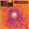 |
Fig. B.1 Slice of the gaseous grid close to the central potential. The outer dotted line shows the refinement region defined by rrefine, while the inner dashed line depicts the softening length of the gravitational potential. |
References
- Ardila, D. R., Golimowski, D. A., Krist, J. E., et al. 2007, ApJ, 665, 512 [NASA ADS] [CrossRef] [Google Scholar]
- Avenhaus, H., Quanz, S. P., Schmid, H. M., et al. 2014, ApJ, 781, 87 [NASA ADS] [CrossRef] [Google Scholar]
- Baraffe, I., Chabrier, G., & Gallardo, J. 2009, ApJ, 702, L27 [NASA ADS] [CrossRef] [Google Scholar]
- Baraffe, I., Vorobyov, E., & Chabrier, G. 2012, ApJ, 756, 118 [NASA ADS] [CrossRef] [Google Scholar]
- Bate, M. R. 2018, MNRAS, 475, 5618 [NASA ADS] [CrossRef] [Google Scholar]
- Benisty, M., Stolker, T., Pohl, A., et al. 2017, A&A, 597, A42 [NASA ADS] [CrossRef] [EDP Sciences] [Google Scholar]
- Blitz, L. 1993, in Protostars and Planets III, eds. E. H. Levy, & J. I. Lunine, 125 [Google Scholar]
- Bondi, H. 1952, MNRAS, 112, 195 [NASA ADS] [CrossRef] [MathSciNet] [Google Scholar]
- Bondi, H., & Hoyle, F. 1944, MNRAS, 104, 273 [NASA ADS] [CrossRef] [Google Scholar]
- Brauer, F., Henning, T., & Dullemond, C. P. 2008, A&A, 487, L1 [NASA ADS] [CrossRef] [EDP Sciences] [Google Scholar]
- DeWarf, L. E., Sepinsky, J. F., Guinan, E. F., Ribas, I., & Nadalin, I. 2003, ApJ, 590, 357 [NASA ADS] [CrossRef] [EDP Sciences] [Google Scholar]
- Dubinski, J., Narayan, R., & Phillips, T. G. 1995, ApJ, 448, 226 [NASA ADS] [CrossRef] [Google Scholar]
- Dullemond, C. P., Küffmeier, M., Goicovic, F., et al. 2019, A&A, 628, A20 [NASA ADS] [CrossRef] [EDP Sciences] [Google Scholar]
- Dunham, M. M., Evans, II, N. J., Terebey, S., Dullemond, C. P., & Young, C. H. 2010, ApJ, 710, 470 [NASA ADS] [CrossRef] [Google Scholar]
- Evans, II, N. J., Dunham, M. M., Jørgensen, J. K., et al. 2009, ApJS, 181, 321 [NASA ADS] [CrossRef] [Google Scholar]
- Falgarone, E., Hily-Blant, P., & Levrier, F. 2004, Ap&SS, 292, 89 [NASA ADS] [CrossRef] [Google Scholar]
- Federrath, C., Banerjee, R., Seifried, D., Clark, P. C., & Klessen, R. S. 2011, IAU Symp., 270, 425 [NASA ADS] [Google Scholar]
- Field, G. B., Goldsmith, D. W., & Habing, H. J. 1969, ApJ, 155, L149 [NASA ADS] [CrossRef] [Google Scholar]
- Frimann, S., Jørgensen, J. K., Dunham, M. M., et al. 2017, A&A, 602, A120 [NASA ADS] [CrossRef] [EDP Sciences] [Google Scholar]
- Fukagawa, M., Hayashi, M., Tamura, M., et al. 2004, ApJ, 605, L53 [NASA ADS] [CrossRef] [Google Scholar]
- Goicovic, F. G., Springel, V., Ohlmann, S. T., & Pakmor, R. 2019, MNRAS, 487, 981 [NASA ADS] [CrossRef] [Google Scholar]
- Grady, C. A., Woodgate, B., Bruhweiler, F. C., et al. 1999, ApJ, 523, L151 [NASA ADS] [CrossRef] [Google Scholar]
- Grady, C. A., Polomski, E. F., Henning, T., et al. 2001, AJ, 122, 3396 [NASA ADS] [CrossRef] [Google Scholar]
- Greif, T. H., Springel, V., White, S. D. M., et al. 2011, ApJ, 737, 75 [NASA ADS] [CrossRef] [Google Scholar]
- Haisch, Jr. K. E., Lada, E. A., & Lada, C. J. 2001, ApJ, 553, L153 [NASA ADS] [CrossRef] [Google Scholar]
- Haugbølle, T., Padoan, P., & Nordlund, Å. 2018, ApJ, 854, 35 [NASA ADS] [CrossRef] [Google Scholar]
- Heiles, C. 1997, ApJ, 481, 193 [NASA ADS] [CrossRef] [Google Scholar]
- Hoyle, F., & Lyttleton, R. A. 1939, Proc. Camb. Philos. Soc., 35, 405 [Google Scholar]
- Jensen, S. S., & Haugbølle, T. 2018, MNRAS, 474, 1176 [NASA ADS] [CrossRef] [Google Scholar]
- Jørgensen, J. K., Visser, R., Williams, J. P., & Bergin, E. A. 2015, A&A, 579, A23 [NASA ADS] [CrossRef] [EDP Sciences] [Google Scholar]
- Kenyon, S. J., Hartmann, L. W., Strom, K. M., & Strom, S. E. 1990, AJ, 99, 869 [NASA ADS] [CrossRef] [Google Scholar]
- Keppler, M., Benisty, M., Müller, A., et al. 2018, A&A, 617, A44 [NASA ADS] [CrossRef] [EDP Sciences] [Google Scholar]
- Klessen, R. S., & Hennebelle, P. 2010, A&A, 520, A17 [NASA ADS] [CrossRef] [EDP Sciences] [Google Scholar]
- Kuffmeier, M., Haugbølle, T., & Nordlund, Å. 2017, ApJ, 846, 7 [NASA ADS] [CrossRef] [Google Scholar]
- Kuffmeier, M., Frimann, S., Jensen, S. S., & Haugbølle, T. 2018, MNRAS, 475, 2642 [NASA ADS] [CrossRef] [Google Scholar]
- Kuffmeier, M., Calcutt, H., & Kristensen, L. E. 2019, A&A, 628, A112 [NASA ADS] [CrossRef] [EDP Sciences] [Google Scholar]
- Kunitomo, M., Guillot, T., Takeuchi, T., & Ida, S. 2017, A&A, 599, A49 [NASA ADS] [CrossRef] [EDP Sciences] [Google Scholar]
- Langer, W. D., Velusamy, T., Kuiper, T. B. H., et al. 1995, ApJ, 453, 293 [NASA ADS] [CrossRef] [Google Scholar]
- Larson, R. B. 1969, MNRAS, 145, 271 [NASA ADS] [CrossRef] [Google Scholar]
- Larson, R. B. 1981, MNRAS, 194, 809 [NASA ADS] [CrossRef] [Google Scholar]
- Li, Z.-Y., Krasnopolsky, R., & Shang, H. 2011, ApJ, 738, 180 [NASA ADS] [CrossRef] [Google Scholar]
- Liu, H. B., Takami, M., Kudo, T., et al. 2016, Sci. Adv., 2, e1500875 [Google Scholar]
- Liu, H. B., Dunham, M. M., Pascucci, I., et al. 2018, A&A, 612, A54 [NASA ADS] [CrossRef] [EDP Sciences] [Google Scholar]
- Mac Low, M.-M., & Klessen, R. S. 2004, Rev. Mod. Phys., 76, 125 [NASA ADS] [CrossRef] [Google Scholar]
- Machida, M. N., & Matsumoto, T. 2011, MNRAS, 413, 2767 [NASA ADS] [CrossRef] [Google Scholar]
- Machida, M. N., Inutsuka, S.-i., & Matsumoto, T. 2010, ApJ, 724, 1006 [NASA ADS] [CrossRef] [Google Scholar]
- Mamajek, E. E. 2009, AIP Conf. Ser., 1158, 3 [Google Scholar]
- Manara, C. F., Morbidelli, A., & Guillot, T. 2018, A&A, 618, L3 [NASA ADS] [CrossRef] [EDP Sciences] [Google Scholar]
- Marino, S., Perez, S., & Casassus, S. 2015, ApJ, 798, L44 [NASA ADS] [CrossRef] [Google Scholar]
- Masson, J., Chabrier, G., Hennebelle, P., Vaytet, N., & Commerçon B. 2016, A&A, 587, A32 [NASA ADS] [CrossRef] [EDP Sciences] [Google Scholar]
- Mestel, L., & Spitzer, Jr. L. 1956, MNRAS, 116, 503 [NASA ADS] [CrossRef] [Google Scholar]
- Mignone, A., Bodo, G., Massaglia, S., et al. 2007, ApJS, 170, 228 [Google Scholar]
- Moeckel, N., & Throop, H. B. 2009, ApJ, 707, 268 [NASA ADS] [CrossRef] [Google Scholar]
- Mulders, G. D., Pascucci, I., & Apai, D. 2015, ApJ, 814, 130 [NASA ADS] [CrossRef] [Google Scholar]
- Nakajima, T., & Golimowski, D. A. 1995, AJ, 109, 1181 [NASA ADS] [CrossRef] [Google Scholar]
- Nixon, C. J., King, A. R., & Pringle, J. E. 2018, MNRAS, 477, 3273 [NASA ADS] [CrossRef] [Google Scholar]
- Offner, S. S. R., Kratter, K. M., Matzner, C. D., Krumholz, M. R., & Klein, R. I. 2010, ApJ, 725, 1485 [NASA ADS] [CrossRef] [Google Scholar]
- Padoan, P., & Nordlund, Å. 2002, ApJ, 576, 870 [Google Scholar]
- Padoan, P., Haugbølle, T., & Nordlund, Å. 2014, ApJ, 797, 32 [NASA ADS] [CrossRef] [Google Scholar]
- Pakmor, R., Springel, V., Bauer, A., et al. 2016, MNRAS, 455, 1134 [NASA ADS] [CrossRef] [Google Scholar]
- Seifried, D., Banerjee, R., Pudritz, R. E., & Klessen, R. S. 2013, MNRAS, 432, 3320 [NASA ADS] [CrossRef] [Google Scholar]
- Springel, V. 2010, MNRAS, 401, 791 [NASA ADS] [CrossRef] [Google Scholar]
- Stolker, T., Dominik, C., Avenhaus, H., et al. 2016, A&A, 595, A113 [NASA ADS] [CrossRef] [EDP Sciences] [Google Scholar]
- Tannirkulam, A., Monnier, J. D., Harries, T. J., et al. 2008, ApJ, 689, 513 [NASA ADS] [CrossRef] [Google Scholar]
- Tomida, K., Okuzumi, S., & Machida, M. N. 2015, ApJ, 801, 117 [NASA ADS] [CrossRef] [Google Scholar]
- van den Ancker, M. E., de Winter, D., & Tjin A Djie, H. R. E. 1998, A&A, 330, 145 [NASA ADS] [Google Scholar]
- Vorobyov, E. I., & Basu, S. 2010, ApJ, 719, 1896 [NASA ADS] [CrossRef] [Google Scholar]
- Whipple, F. L. 1972, in From Plasma to Planet, ed. A. Elvius (New York: Wiley Interscience Division), 211 [Google Scholar]
- Wijnen, T. P. G., Pols, O. R., Pelupessy, F. I., & Portegies Zwart, S. 2016, A&A, 594, A30 [NASA ADS] [CrossRef] [EDP Sciences] [Google Scholar]
- Wijnen, T. P. G., Pols, O. R., Pelupessy, F. I., & Portegies Zwart, S. 2017a, A&A, 602, A52 [NASA ADS] [CrossRef] [EDP Sciences] [Google Scholar]
- Wijnen, T. P. G., Pelupessy, F. I., Pols, O. R., & Portegies Zwart, S. 2017b, A&A, 604, A88 [NASA ADS] [CrossRef] [EDP Sciences] [Google Scholar]
- Wurster, J., Bate, M. R., & Price, D. J. 2018, MNRAS, 475, 1859 [NASA ADS] [CrossRef] [Google Scholar]
- Wurster, J., Bate, M. R., & Price, D. J. 2019, MNRAS, 489, 1719 [NASA ADS] [CrossRef] [Google Scholar]
http://plutocode.ph.unito.it version 4.
All Tables
All Figures
|
Fig. 1 Illustration of the column density in the planes perpendicular to the orientation of the angular momentum vector for the setups of the adiabatic run A1 (upper panels) and the isothermal run I1 (lower panels) at times (t0 = 0, t1 = 4 tdyn, t2 = 8 tdyn, and t3 = 16 tdyn. |
| In the text | |
|
Fig. 2 Illustration of the column density in the three planes of the coordinate system (left panels: xy, middle panels: yz, right panels: xz) for the setups of the isothermal runs after 10 dynamical times (t = 10 tdyn). Panels in odd rows correspond to pure isothermal runs and panels in even rows correspond to the cases with stellar irradiation. |
| In the text | |
|
Fig. 3 Column density in the planes perpendicular to the orientation of the angular momentum vector for runs IrrI1_t0, IrrI1_t500, IrrI1_t1000, and IrrI1_t at times (t0 = 0, t1 = 4 tdyn, t2 = 8 tdyn, and t3 = 16 tdyn. |
| In the text | |
|
Fig. 4 Evolution of captured mass and accreted mass for altogether 14 runs.Upper panels: amount of mass within 1000 au from the central potential. Lower panels: corresponding amount of accreted mass. The line style and color is used consistently for the upper and lower plots. Left panels: A1 (blue solid), A1_t (green dashed), A1_t_nw (red dotted), I1 (cyan solid), I1_t (purple dashed), I1_t_nw (black dotted), and IrrI1_t (yellow solid); right panels: A2 (blue solid), A2_t (green dashed), A2_t_nw (red dotted), I2 (cyan solid), I2_t (purple dashed), I2_t_nw (black dotted), and IrrI2_t (yellow solid). |
| In the text | |
|
Fig. 5 Velocity profiles at t = 16 tdyn for the different runs. Left panel: A1 (blue solid), A1_t (green dashed), A1_t_nw (red dotted), I1 (cyan solid), I1_t (purple dashed), I1_t_nw (black dotted), and IrrI1_t (yellow solid); middle panel: A2 (blue solid), A2_t (green dashed), A2_t_nw (red dotted), I2 (cyan solid), I2_t (purple dashed), I2_t_nw (black dotted), and IrrI2_t (yellow solid); right panel: A3 (blue solid), A3_t (green dashed), A3_t_nw (red dotted), I3 (cyan solid), I3_t (purple dashed), I3_t_nw (black dotted), and IrrI3_t (yellow solid). The black solid line corresponds to the Keplerian velocity
|
| In the text | |
|
Fig. 6 Column density in the planes perpendicular to the orientation of the angular momentum vector for run IrrI1_t at different times. Upper panel, from left to right: t1 = 4 tdyn, t2 = 8 tdyn, t3 = 12 tdyn, t4 = 16, t5 = 20 tdyn, and lower panel, from left to right: t6 = 24 tdyn, t7 = 28 tdyn, t8 = 32 tdyn, t9 = 36 tdyn and at the end of the simulation t10 = 39 tdyn. |
| In the text | |
|
Fig. 7 Azimuthally averaged column density in the planes. The column densities are computed perpendicular to the orientation of the angular momentum vector for run IrrI1_t. The profiles correspond to the times represented in the projection plots in Fig. 6. Left panel: t1 = 4 tdyn (blue solid), t2 = 8 tdyn (green dashed), t3 = 12 tdyn (red dotted),t4 = 16 (cyan solid), and t5 = 20 tdyn (purple dashed); right panel: t6 = 24 tdyn (blue solid), t7 = 28 tdyn (green dashed), t8 = 32 tdyn (red dotted),t9 = 36 tdyn (cyan solid), and t10 = 39 tdyn (purple dashed). The red dashed line corresponds to the profile of the MMSN,
|
| In the text | |
|
Fig. A.1 Slice of the initial setup of the grid. This illustrate our procedure to guarantee a modest transition between the highly resolved cloud (resolution not shown) and the coarsely resolved background. |
| In the text | |
|
Fig. B.1 Slice of the gaseous grid close to the central potential. The outer dotted line shows the refinement region defined by rrefine, while the inner dashed line depicts the softening length of the gravitational potential. |
| In the text | |
Current usage metrics show cumulative count of Article Views (full-text article views including HTML views, PDF and ePub downloads, according to the available data) and Abstracts Views on Vision4Press platform.
Data correspond to usage on the plateform after 2015. The current usage metrics is available 48-96 hours after online publication and is updated daily on week days.
Initial download of the metrics may take a while.