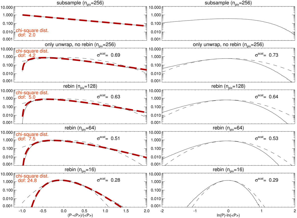
Normalized frequency distribution functions of the normalized synthetic power at k_pix = 21 (ℓ = 492, black solid lines): top panels are for the subsampled power and the second panels are the unwrapped power without further smoothing, while the lower panels are for the rebinned powers. Left panels: (P − ⟨P⟩)/⟨P⟩, and right panels: lnP − ln⟨P⟩, where ⟨⟩ indicates the expectation value (model). The input model of the power is isotropized (q_i, n = 0 for 3 ≤ i ≤ 6 for all n and q_i, b = 0 for i = 2, 3) but otherwise it is the same as the model with the parameters given in Table C.2. For this plot, we use 50 realizations for the top two rows and 500 realizations for the rebinned data (lower three rows). The black dashed lines on the lower four panels are the Gaussian function centered at zero whose width is the standard deviation of the samples (shown on the panels). This validates our approximation of the distribution function of the logarithm of the power by the Gaussian function. The thick red dashed curves on the left panels are the chi-square distribution function of various degrees of freedom. The degree of freedom (d.o.f.) for each distribution is determined from the standard deviation of each set of normalized power. See the text for details.