| Issue |
A&A
Volume 633, January 2020
|
|
|---|---|---|
| Article Number | A87 | |
| Number of page(s) | 7 | |
| Section | Planets and planetary systems | |
| DOI | https://doi.org/10.1051/0004-6361/201936604 | |
| Published online | 15 January 2020 | |
Magnetohydrodynamic simulations of a Uranus-at-equinox type rotating magnetosphere
1
Institut de Recherche en Astrophysique et Planétologie (IRAP), CNRS, CNES, Université de Toulouse, UPS,
Toulouse,
France
e-mail: This email address is being protected from spambots. You need JavaScript enabled to view it.
2
LESIA, Observatoire de Paris, Université PSL, CNRS, Sorbonne Université, Université de Paris,
5 place Jules Janssen,
92195 Meudon,
France
Received:
30
August
2019
Accepted:
18
November
2019
Abstract
Context. As proven by measurements at Uranus and Neptune, the magnetic dipole axis and planetary spin axis can be off by a large angle exceeding 45°. The magnetosphere of such an (exo-)planet is highly variable over a one-day period and it does potentially exhibit a complex magnetic tail structure. The dynamics and shape of rotating magnetospheres do obviously depend on the planet’s characteristics but also, and very substantially, on the orientation of the planetary spin axis with respect to the impinging, generally highly supersonic, stellar wind.
Aims. On its orbit around the Sun, the orientation of Uranus’ spin axis with respect to the solar wind changes from quasi-perpendicular (solstice) to quasi-parallel (equinox). In this paper, we simulate the magnetosphere of a fictitious Uranus-like planet plunged in a supersonic plasma (the stellar wind) at equinox. A simulation with zero wind velocity is also presented in order to help disentangle the effects of the rotation from the effects of the supersonic wind in the structuring of the planetary magnetic tail.
Methods. The ideal magnetohydrodynamic (MHD) equations in conservative form are integrated on a structured spherical grid using the Message-Passing Interface-Adaptive Mesh Refinement Versatile Advection Code (MPI-AMRVAC). In order to limit diffusivity at grid level, we used background and residual decomposition of the magnetic field. The magnetic field is thus made of the sum of a prescribed time-dependent background field B0(t) and a residual field B1(t) computed by the code. In our simulations, B0(t) is essentially made of a rigidly rotating potential dipole field.
Results. The first simulation shows that, while plunged in a non-magnetised plasma, a magnetic dipole rotating about an axis oriented at 90° with respect to itself does naturally accelerate the plasma away from the dipole around the rotation axis. The acceleration occurs over a spatial scale of the order of the Alfvénic co-rotation scale r*. During the acceleration, the dipole lines become stretched and twisted. The observed asymptotic fluid velocities are of the order of the phase speed of the fast MHD mode. In two simulations where the surrounding non-magnetised plasma was chosen to move at supersonic speed perpendicularly to the rotation axis (a situation that is reminiscent of Uranus in the solar wind at equinox), the lines of each hemisphere are symmetrically twisted and stretched as before. However, they are also bent by the supersonic flow, thus forming a magnetic tail of interlaced field lines of opposite polarity. Similarly to the case with no wind, the interlaced field lines and the attached plasma are accelerated by the rotation and also by the transfer of kinetic energy flux from the surrounding supersonic flow. The tailwards fluid velocity increases asymptotically towards the externally imposed flow velocity, or wind. In one more simulation, a transverse magnetic field, to both the spin axis and flow direction, was added to the impinging flow so that magnetic reconnection could occur between the dipole anchored field lines and the impinging field lines. No major difference with respect to the no-magnetised flow case is observed, except that the tailwards acceleration occurs in two steps and is slightly more efficient. In order to emphasise the effect of rotation, we only address the case of a fast-rotating planet where the co-rotation scale r* is of the order of the planetary counter-flow magnetopause stand-off distance rm. For Uranus, r*≫ rm and the effects of rotation are only visible at large tailwards distances r ≫ rm.
Key words: planet-star interactions / methods: numerical / plasmas / magnetohydrodynamics (MHD)
© L. Griton and F. Pantellini 2020
 Open Access article, published by EDP Sciences, under the terms of the Creative Commons Attribution License (http://creativecommons.org/licenses/by/4.0), which permits unrestricted use, distribution, and reproduction in any medium, provided the original work is properly cited.
1 Introduction
Uranus’ magnetosphere was explored in situ by the Voyager II spacecraft during its January 1986 flyby. Magnetic field measurements unveiled a dipole field strength of  , where rU is the radius of Uranus, confirming the prediction of Siscoe (1971) that Uranus’ composition would be compatible with the presence of an intrinsic magnetic field, strong enough to sustain a planetary magnetosphere. Thus, not surprisingly, during inbound flight from upstream, Voyager II successively encountered the bow shock and the magnetopause at 23.3 rU and 18 rU from the planet’s centre, respectively (Ness et al. 1986). The nearly sunward pointing spin axis orientation of the planet at the time of Voyager’s flyby (solstice configuration) offered a unique opportunity to observe a planetary magnetosphere with one of the poles pointing towards the Sun (e.g. Voight et al. 1983). Besides the exotic orientation of its spin axis with respect to the ecliptic plane, Voyager II also revealed an unexpected large angle of 59° between the spin axis and magnetic axis (Ness et al. 1986; Connerney et al. 1987). Radio and magnetic field measurements by Voyager II also allowed one to measure, with unprecedented precision, the rotation period of Uranus to be relatively fast, 17.24± 0.01 h, when compared to the magnetospheric relaxation time (Desch et al. 1986). As a consequence, the magnetosphere of Uranus is highly variable, with both diurnal and seasonal variations (Lepping 1994; Schulz & McNab 1996; Cao & Paty 2017).
Based on 15.2 h of measurement of the magnetic field orientation whilst Voyager II was inside the nightside magnetosheath, Behannon et al. (1987) estimated that the magnetic field lines composing the north and south tail lobes present a helical twist of pitch α = 5.5° ± 3.0°. Assuming acylinder-shaped tailwards magnetopause surface with an inferred radius of 42 rU, the wavelength of the twist turns out to be of the order of λ = 2π × 42 rU∕tanα = 2740 rU (Behannon et al. 1987).
Following Voyager’s observations, 3D magnetohydrodyna- mic (MHD) simulations of Uranus or Uranus-like magnetospheres in a solstice configuration have been published (Tóth et al. 2004; Cao & Paty 2017; Griton et al. 2018). In particular, the Tóth et al. (2004) simulation seems to indicate that the wavelength of the twist inferred by Behannon et al. (1987), which was based on the sparse data collected by Voyager II during its short flight through Uranus’ tail, is probably in excess by a factor of three (Tóth et al. (2004) find λ = 900 rU). The equinox configuration, however, has been addressed in just one paper by Cowley (2013) with the guiding idea to help understand the distant UV auroral observations by Lamy et al. (2012). Cao & Paty (2017) essentially concentrate on the dayside structure of the magnetosphere as a function of both the seasons and the planet’s phase, and they do not focus as much on the physical effects of rotation. In this paper we present a detailed study of the role of the planetary rotation on the tailwards acceleration of the magnetospheric plasma.
2 Methods
2.1 Simplifications
In this paper, we concentrate on the role of planetary rotation for a Uranus-like configuration at equinox. The purpose here is not to produce faithful simulations of Uranus but rather to investigate the effects of rotation on a Uranus-like dipole plunged in a supersonic flow (stellar wind). Besides the fact that the rotation period and the dipole intensities are not the same as those of Uranus (see Table 1 below), we also simplify the orientations of the relevant axis and directions as shown in Fig. 1. The main approximations are as follows: (1) the magnetic axis goes through the planet’s centre, (2) the spin axis is at 90° with respect to the magnetic axis, and (3) the spin axis is perpendicular to the flow direction. In this paper we assume that the planetary field is strictly dipolar. This is a rather minor simplification as the fractional contribution of higher order terms (quadrupolar, octopolar, etc.) at a planet’s surface is generally small and, by definition, rapidly decreasing with distance.
Main parameters of the simulations discussed in the paper.
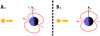 |
Fig. 1 Axis orientation of the planet Uranus at equinox (A) and simplified version used in this paper (B). Red arrow is for the magnetic axis and black arrow for the planetary spin axis. Yellow thick arrow indicates the solar wind propagation direction. |
2.2 Simulations set-up and parameters
Four simulations are discussed in this paper (see Table 1). In the first one (run 1), a magnetic dipole that is plunged in a resting plasma rotates about an axis perpendicular to itself. In the other three simulations (runs 2 to 4), the angle between the spin axis and the magnetic dipole is also 90°; however, the surrounding plasma flows at supersonic speed and perpendicularly to the rotation axis. Such a configuration is reminiscent of the planet Uranus at equinox. In runs 2 and 3, the angular velocity is roughly two times smaller than in run 4. Run 3 differs from run 2 in that a constant magnetic field has been added into the flow. The reference frame of the simulation is a right-handed Cartesian frame with the z-axis pointing against the solar wind flow. The spin axis points towards the positive x-axis so that it is orthogonal to the flow. The y-axis completes the right-handed coordinate system. We do arbitrarily assume that at t = 0, the magnetic dipole is oriented parallel to the z-axis. The magnetic dipole is located at r = 0. We used a modified version of the MHD module of the Message-Passing Interface-Adaptive Mesh Refinement Versatile Advection Code (MPI-AMRVAC; Keppens et al. 2012), allowing the use of a time-dependent pre-defined background magnetic field. In our case, the background field is a rotating magnetic dipole, as discussed in Griton et al. (2018). In the case of the non-zero intensity of the magnetic field BI in the impinging plasma (as for run 3, see Table 1), the latter was added to the background field. As in previous simulations of planetary magnetospheres (see Pantellini et al. 2015, Chap. 2), we used a two-step Lax-Friedrichs type scheme (called TVDLF in MPI-AMRVAC) associated with a gradient limiter minmod.
The simulation domain is a spherical shell, extending from r = rmin (inner boundary) to r = rmax (outer boundary). We use a structured spherical grid with regularly spaced grid points in θ and ϕ. In the radial direction r, we use either a constant or an outwards geometrically growing grid size as detailed in Table 1. MPI-AMRVAC allows for local mesh refinement, but this was not necessary. Boundary conditions at both inner and outer boundaries are the same as in Griton et al. (2018).
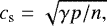
For convenience, and to avoid specialisation, dimensionless quantities are used throughout the paper. Spatial dimensions are normalised to the radius rmin of the innerboundary of the simulation domain (the planetary radius throughout the paper). The mass isnormalised to the average molecular mass so that in normalised units, mass density ρ and number density n are interchangeable, that is, ρ = n. Velocities are normalised to the adiabatic sound speed in the surrounding, unperturbed, plasma. Densities are also normalised to the value in the surrounding plasma. As a consequence, from the expression of the adiabatic sound speed  , it follows that the dimensionless pressure in the unperturbed plasma is 1∕γ. The vacuumpermeability μ0 is coherently set to unity so that in terms of dimensionless quantities, the Alfvén speed is
  and the plasma beta β = 2p∕B2. The latter is equivalent to the normalisation independent expression
 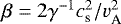 .
.
3 Rotating planetary dipole plunged in a resting plasma
In a vacuum a dipole rotates rigidly for distances to the rotation axis r ≪ c∕Ω, where c is the speed of light and Ω the angular velocity of the rotation. On the other hand, if the dipole is plunged in a plasma and rotation is started at t = 0 for example, the plasma along any given field line is set in motion perpendicularly to the plane of the field line by an Alfvén wave emitted at the inner boundary. In that case, the rigid rotation approximation breaks down at much smaller distances r, where the Alfvén velocity and the co-rotation velocity are of the same order. At such distances, the effect of rotation is the one that is schematically illustrated in Fig. 2, which shows the deformation of the field lines under the effect of the centrifugal force, resulting from the fluid that is set in motion perpendicularly to the plane of the field line.
Assuming the plasma temperature is low enough so that only the Lorentz force has to be considered, one may immediately conclude that the effect of the deformation of the lines from position 1 to 2, as shown in Fig. 2, is the reduction of their curvature and thus their magnetic tension (directed towards the centre) along the rotation axis. On the other hand, the displacement of the lines from position 1 to 2 does not change the magnetic pressure gradient along the rotation axis; therefore, an unbalanced, net outward-directed force arises (blue arrow).
The acceleration of the plasma along the rotation axis for a rotating dipole in an initially motionless plasma can be observed in simulation 1 (see Table 1). Figure 3 shows a snapshot of the simulation at time t = 41.00, shortly afterthe end of the fifth rotation. Only half of the system is shown, the other half is its symmetric replica. By that time and given that there is no magnetic field in the surrounding plasma, the system has reached a stationary state in the frame of the rotatingdipole. In the left panel of the figure, four sample field lines of various length passing through the x axis are shown. As the system is stationary, each line may be interpreted as the same line at different times. The fluid velocity profile vx (x) in the right panel shows that the plasma and thus the field lines are expelled along the rotation axis at increasingly high speeds, eventually exceeding the fast-mode velocity. Even though the profiles may not be strictly independent of the conditions at the outer boundary, the simulation clearly shows that a dipole, which rotates about an axis that is perpendicular to itself, is an efficient plasma accelerator. Since magnetic field lines expand from the dipole’s centre, magnetic flux has to be steadily injected at the inner boundary.
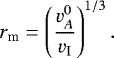
The characteristic length r* over which acceleration occurs, which is also of the order of the co-rotation distance, can be evaluated very roughly by assuming a constant plasma density and a magnetic field intensity decrease ∝ r−3 (dipole field). This leads to
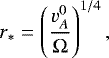 (1)
(1)
where 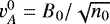 is the dipole equatorial Alfvèn speed at r = 1. Given the parameters of simulation 1, one obtains r*≃ 2.8. The same expression gives r*~ 30–50 for the real Uranus.
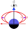 |
Fig. 2 Field line (1) corresponds to the equilibrium position of a non-rotating potential dipole plunged in a uniform plasma. If the dipole is set into rotation about an axis perpendicular to itself, centrifugal forces (violet arrows) displace the field line from position 1–2. Simultaneously, and in assuming that the temperature effects can be neglected for simplicity purposes, a net outward-directed Lorentz force arises (blue arrow) and then accelerates the plasma in the x direction (the spin axis). One may note that the picture is pertinent provided that the Alfvén travel time from one footpoint to the other of the field line is much shorter than the rotation period. |
4 Rotating planetary dipole plunged in a supersonic plasma flow
When the rotating dipole is immersed in a supersonic plasma, such as Uranus in the solar wind, a new scale length arises in addition to r* defined by Eq. (1). This new scale length is the stand-off distance rm of the planetary magnetopause in the direction opposing the supersonic flow. The stand-off distance can be estimated to lowest order by equilibrating the dynamic pressure of the plasma flow  and the planetary magnetic pressure at that distance 0.5B2(rm). Again in assuming a B ∝ r−3 dependence and a uniform density of n = nI in the whole system, one has:
 (2)
(2)
With the parameters of Table 1, the stand-off distance can thus be estimated as  for all simulations where vI≠0.
In the case of an extremely slowly rotating planet rm ≪ r*, the structure of the magnetosphere in the vicinity of the planet is essentially unaffected by rotation and no twist of planet connected field lines is expected. For fast-rotating planets where rm ≫ r*, field lines are completely twisted up before reaching rm, which thus becomes meaningless. In the next sections, we discuss simulations where both distances are comparable rm ~ r*~ 4. Simulations are advanced in time long enough for the initial conditions to be forgotten and the system to become strictly periodic. One may note that due to the fact that the impinging flow is perpendicular to the spin axis, there is no frame in which the system reaches a stationary state as in the case of the rotating dipole in a plasma at rest.
4.1 Unmagnetised supersonic flow
Let us first focus on the simplest case where the impinging supersonic flow is unmagnetised. Under such circumstances, no magnetic connection can be established between the flow and the planet: a planetary field line does necessarily start and end on the planet’s surface. Figure 4 shows a snapshot of run 2. As for run 1, the system is symmetric with respect to the spin equator. As for the free rotating dipole of Fig. 3, the field lines are seen to be twisted by the rotation. At the same time, since rm ~ r*, the field lines are bended in the direction of the flow. Even though the profiles in the right panels of Fig. 4 are not taken along the spin axis as in Fig. 3, but along a more pertinent axis starting from the centre of the planet towards downstream, the overall picture is qualitatively the same in both simulations. Indeed, in both simulations the fluid velocity is accelerated to high velocities over a spatial scale coherent with the above estimates of r*. The fact that acceleration is steeper in run 2 (where r* = 4.8) with respect to run 1 (where r* = 2.8) can be due to many different reasons. First, even though the impinging plasma and the plasma contained in the planetary flux tubes do not mix in run 2, the impinging flow transmits an additional kinetic energy flux in places where the fluid flow and magnetic field lines are not aligned. This continuous transfer of kinetic flux actually drives the asymptotic velocity towards vI = 20. Second, as previously stated, the plotted profiles are taken along different paths. Third, some minor effects may be due to the different spatial resolutions, different domain sizes, and different plasma conditions near the outer boundaries. We shall mention here that with no rotation and in the context of an ideal MHD with zero resistivity and zero viscosity, a stationary state is expected to form where the plasma magnetically connected to the planetary field is at rest while the impinging supersonic plasma flows around the magnetospheric obstacle. Magnetic flux does not escape from the planet in that extreme limit.
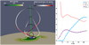 |
Fig. 3 Snapshot from simulation 1 after reaching the stationary regime. On the left panel, four field lines are shown and colour-coded according to the field-aligned Alfvén speed travel time from the apex of the line divided by the rotation period. Field lines are increasingly twisted as field-aligned Alfvén travel time increases. As the system is symmetric with respect to the equatorial rotation plane, only the upper hemisphere is shown. Neither magnetic field lines nor streamlines cross the equator. Colour contours of the fluid velocity in the equatorial plane illustrate the modulation of the plasma flow by the rotating dipole as well as the field lines lagging effect at large radial distances where the co-rotation velocity exceeds the Alfvén velocity. On the right panel, the flow velocity
vx, the sound speed |
4.2 Magnetised supersonic flow
Run 3 only differs with respect to run 2 by the addition of a uniform magnetic field BI in the impinging flow. The orientation of the impinging magnetic field (IMF) is perpendicular to both the spin axis and the flow direction so that the equatorial plane remains a plane of symmetry. Figure 5 shows a snapshot of the simulation at the same planetary rotation phase as for the unmagnetised case of Fig. 4. Differences are rather minor but visible. First, magnetic reconnection between the planetary field and the magnetic field in the impinging plasma becomes possible, as illustrated by one of the three sample field lines in the left panel of the figure (indicated by the red arrow on Fig. 5). Second, the acceleration of the plasma downstream of the planet is not as smooth as in the unmagnetised case. Indeed, while for − z < 8 where only closed planetary field lines are present, the profiles are nearly identical in the two simulations. This is not the case in the interval − z ∈ [8, 13], where the acceleration of the plasma is slower in run 3, as compared to run 2. This effect is clearly due to the reconnection between the planetary magnetic field and the IMF. At larger distances, for − z > 13, all magnetic field lines are disconnected from the planet and the acceleration of the flow increases again due to the effect of the relaxation of newly disconnected magnetic field lines. As a result, at − z = 30 the flow velocity is already of the order of vz = 16.8 against 15.5 only for the unmagnetised simulation of Fig. 4. We note that in this situation, magnetic reconnection participates in the acceleration process, which is therefore more efficient than in the unmagnetised case discussed in the previous section.
4.3 Fast-rotating planetary dipole in unmagnetised supersonic flow
Simulation 4 is mainly characterised by a rotation that is more than twice as fast than in runs 2 and 3 and has more grid cells in the radialdirection. Combined with the fact that the radial extension of the cells is constant as opposed to in simulations 1–3 in which it increases geometrically with r, one can deduce that the spatial resolution is higher at large distances r. The downside of the constant cell size in the radial direction is that the cells become stretched in θ and ϕ with increasing r. It should be noted that r*∝ Ω−1∕4 implies that Ω, only marginally affects r* and therefore does not modify in a significant way the near planet acceleration of the plasma observed in Figs. 4and 5. On the other hand, since the twisting of the field lines in the downstream region must be periodic with a wavelength λ ≤ 2πvI∕Ω, it follows that λ ≃ 20 for run 4 so that at least two periods should be observable. The twisting of sample field lines from both poles of the dipole is neatly visible in Fig. 6. Except for the orientation of the spin and magnetic axes, in addition to the absence of IMF, run 4 is identical to the runs from Griton et al. (2018) reminiscent of Uranus in a “solstice” configuration, with its spin axis aligned with the propagation of the solar wind. In run 4 and as seen in Fig. 6, the wavelength of the magnetic structure only slightly grows over the two observable oscillations, which illustrates the fact that the acceleration mainly occurs close to the planet. Again, the spin equatorial plane x = 0 is a symmetry plane with identical structures in both the upper and lower hemisphere. Also, neither magnetic field lines nor stream lines cross the plane of symmetry. It should be noted that in the absence of an impinging magnetic field and in addition to a 2π∕Ω time periodicity, the system also has a strict π∕Ω periodicity if it is combined with a magnetic field sign reversal (as in run 2). This means that, after a time interval π∕Ω, the exact same top Fig. 6 is recovered with switched colours. Unfortunately, even if some symmetries are preserved for particular orientations of the impinging magnetic field, the ideal picture shown in the top panel of Fig. 6 is not universal.
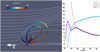 |
Fig. 4 Run 2. Left: selected magnetic field lines coloured according to the sign of the B ⋅ r. Some streamlines are also plotted. Right: − vz component of the flow velocity, sound speed cs, and the fast-mode propagation velocity along the z-axis as a functionof − z. |
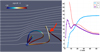 |
Fig. 5 Run 3: same format as Fig. 4. Impinging plasma is magnetised with magnetic field oriented perpendicularly to the plane of the figure. Red arrow indicates a planetary field line having undergone reconnection with a field line transported by the impinging plasma. |
 |
Fig. 6 Sample magnetic field lines for run 4. Colour code indicates whether the magnetic field has positive or negative radial component Br. Sample stream lines are shown in black. |
5 Conclusions
In this paper, we present 3D MHD simulations of a rotating dipole plunged in a supersonic plasma flow. The rotation axis, the dipole axis, and the direction of the impinging flow are selected to be mutually orthogonal, which is reminiscent of the magnetosphere of Uranus at equinox. The objective of the paper is not to provide faithful modelling of a specific rotating planetary magnetosphere as in Tóth et al. (2004) for the case of the slowly rotating Uranus. Since our main objective was to observe the ejection of planetary magnetic flux (and plasma) due to the rotation of the planet, we deliberately accentuate its effect by selecting sufficiently fast angular velocities to force acceleration to occur close to the planet, allowing for the simulation domain to be substantially reduced with respect to the case of Uranus.
In order to disentangle the effect of the rotation from the effect of the supersonic flow surrounding the rotating dipole, we simulated a dipole rotating in a resting plasma unmagnetised plasma first (run 1). The important outcome of this simulation is that the plasma becomes accelerated to at least the fast-mode phase velocity along the rotation axis (see Fig. 3). The spatial scale over which the acceleration occurs is naturally of the order of the co-rotation scale r* for which Eq. (1) provides a rough estimate for a rotating dipolar field. Plunging the rotating dipole into a supersonic flow oriented as mentioned above does not substantially alter the picture at short distances r < r* provided rotation is fast enough, that is, r*≲ rm. Otherwise, the structure of the magnetosphere at distances r ≲ rm would only depend on the actual phase of the planet as in the simulation for Uranus at solstice by Tóth et al. (2004). The impinging flow merely participates in the continued acceleration of the plasma tailwards through a transfer of kinetic energy flux from the incoming flow and/or through magnetic reconnection. In the slow rotation limit r* ≫ rm (in the case of Uranus), which is not explicitly addressed in this paper, the field lines are first stretched and bent under the effect of the impinging flow before being twisted by the effect of rotation. In this case and if reconnection is allowed, the acceleration close to the planet is primarily due to reconnection. However, at larger distances up to order r*, the acceleration due to rotation is still effective, at least as long as the Alfvén travel time along the concerned field lines is shorter than the rotation period 2π∕Ω. This is eventhe case for the slow rotator Uranus, as field line windings tailwards of the planet have been observed by Tóth et al. (2004). We shall conclude by pointing out that the suggestive, and relatively simple, magnetic structure shown in Fig. 6 is much more complex for a non-zero field BI in the impinging plasma, even in the north-south symmetry preserving case where BI is oriented in the y direction. As no spacecraft has ever had the opportunity to explore Uranus’ magnetosphere at equinox, and since no other planet in the Solar System has never found itself in a similar configuration, simulations are the only means for a better understanding of the spatio-temporal structure of such a complex stellar wind-planet interaction.
As explained by Selsis (2007), the definition of habitable planet generally focuses on the ability of the planet to host liquid water on its surface. However, as pointed out by many researchers (see for example the review by Lammer et al. 2009 or Cuntz et al. 2000), the stellar wind-planet interaction can be determinant when it comes to host life on a planetary surface. As planetary magnetic fields from an exoplanet can now be detected from observations (as predicted by Zarka 2007 and recently confirmed by Cauley et al. 2019), the role of planetary magnetospheres is now studied to be included in the definition of the habitable zone, for example, concerning their role in preserving exoplanetary atmospheres from erosion (Rodríguez-Mozos & Moya 2019). Recent modelling of planet-star magnetised interactions (e.g. Strugarek et al. 2014, 2015) focuses on non-rotating planets in synchronised systems, but they also highlight the importance of taking into account fast-rotating planets for future research. The work presented here, along with the previous study from Griton et al. (2018), are together a first step towards a better understanding of the physical mechanisms at work in more complex, highly time-dependent interactions between a star’s wind and a magnetized rotating planet.
Acknowledgements
The Plas@par project is acknowledged for financial support. The work of Léa Griton was supported by the CNES (Centre national d’Etudes Spatiales) and the Observatoire de Paris (contract reference 5100016058).
References
- Behannon, K. W., Lepping, R. P., Sittler, Jr. E. C., et al. 1987, J. Geophys. Res. Space Phys., 92, 15354 [NASA ADS] [CrossRef] [Google Scholar]
- Cao, X., & Paty, C. 2017, J. Geophys. Res. Space Phys., 122, 6318 [Google Scholar]
- Cauley, P. W., Shkolnik, E. L., Llama, J., & Lanza, A. F. 2019, Nat. Astron., 408 [Google Scholar]
- Connerney, J. E. P., Acuña, M. H., & Ness, N. F. 1987, J. Geophys. Res. Space Phys., 92, 15329 [NASA ADS] [CrossRef] [Google Scholar]
- Cowley, S. W. H. 2013, J. Geophys. Res. Space Phys., 118, 2897 [Google Scholar]
- Cuntz, M., Saar, S. H., & Musielak, Z. E. 2000, ApJ, 533, L151 [NASA ADS] [CrossRef] [PubMed] [Google Scholar]
- Desch, M. D., Connerney, J. E. P., & Kaiser, M. L. 1986, Nature, 322, 42 [NASA ADS] [CrossRef] [Google Scholar]
- Griton, L., Pantellini, F., & Meliani, Z. 2018, J. Geophys. Res. Space Phys., 123, 5394 [Google Scholar]
- Keppens, R., Meliani, Z., van Marle, A., et al. 2012, J. Comput. Phys., 231, 718 [Google Scholar]
- Lammer, H., Bredehöft, J. H., Coustenis, A., et al. 2009, A&ARv, 17, 181 [NASA ADS] [CrossRef] [Google Scholar]
- Lamy, L., Prangé, R., Hansen, K. C., et al. 2012, Geophys. Res. Lett., 39 [Google Scholar]
- Lepping, R. P. 1994, Planet. Space Sci., 42, 847 [NASA ADS] [CrossRef] [Google Scholar]
- Ness, N. F., Acuna, M. H., Behannon, K. W., et al. 1986, Science, 233, 85 [NASA ADS] [CrossRef] [PubMed] [Google Scholar]
- Pantellini, F., Griton, L., & Varela, J. 2015, Planet. Space Sci., 112, 1 [NASA ADS] [CrossRef] [Google Scholar]
- Rodríguez-Mozos, J. M., & Moya, A. 2019, A&A, 630, A52 [NASA ADS] [CrossRef] [EDP Sciences] [Google Scholar]
- Schulz, M., & McNab, M. C. 1996, J. Geophys. Res., 101, 5095 [NASA ADS] [CrossRef] [Google Scholar]
- Selsis, F. 2007, Habitability: the Point of View of an Astronomer, eds. M. Gargaud, H. Martin, & P. Claeys (Berlin, Heidelberg: Springer), 199 [Google Scholar]
- Siscoe, G. L. 1971, Planet. Space Sci., 19, 483 [NASA ADS] [CrossRef] [Google Scholar]
- Strugarek, A., Brun, A. S., Matt, S. P., & Réville, V. 2014, ApJ, 795, 86 [NASA ADS] [CrossRef] [Google Scholar]
- Strugarek, A., Brun, A. S., Matt, S. P., & Réville, V. 2015, ApJ, 815, 111 [NASA ADS] [CrossRef] [Google Scholar]
- Tóth, G., KováCs, D., Hansen, K. C., & Gombosi, T. I. 2004, J. Geophys. Res. Space Phys., 109, A11210 [CrossRef] [Google Scholar]
- Voight, G.-H., Hill, T. W., & Dessler, A. J. 1983, ApJ, 266, 390 [NASA ADS] [CrossRef] [Google Scholar]
- Zarka, P. 2007, Planet. Space Sci., 55, 598 [NASA ADS] [CrossRef] [Google Scholar]
All Tables
All Figures
|
Fig. 1 Axis orientation of the planet Uranus at equinox (A) and simplified version used in this paper (B). Red arrow is for the magnetic axis and black arrow for the planetary spin axis. Yellow thick arrow indicates the solar wind propagation direction. |
| In the text | |
|
Fig. 2 Field line (1) corresponds to the equilibrium position of a non-rotating potential dipole plunged in a uniform plasma. If the dipole is set into rotation about an axis perpendicular to itself, centrifugal forces (violet arrows) displace the field line from position 1–2. Simultaneously, and in assuming that the temperature effects can be neglected for simplicity purposes, a net outward-directed Lorentz force arises (blue arrow) and then accelerates the plasma in the x direction (the spin axis). One may note that the picture is pertinent provided that the Alfvén travel time from one footpoint to the other of the field line is much shorter than the rotation period. |
| In the text | |
|
Fig. 3 Snapshot from simulation 1 after reaching the stationary regime. On the left panel, four field lines are shown and colour-coded according to the field-aligned Alfvén speed travel time from the apex of the line divided by the rotation period. Field lines are increasingly twisted as field-aligned Alfvén travel time increases. As the system is symmetric with respect to the equatorial rotation plane, only the upper hemisphere is shown. Neither magnetic field lines nor streamlines cross the equator. Colour contours of the fluid velocity in the equatorial plane illustrate the modulation of the plasma flow by the rotating dipole as well as the field lines lagging effect at large radial distances where the co-rotation velocity exceeds the Alfvén velocity. On the right panel, the flow velocity
vx, the sound speed |
| In the text | |
|
Fig. 4 Run 2. Left: selected magnetic field lines coloured according to the sign of the B ⋅ r. Some streamlines are also plotted. Right: − vz component of the flow velocity, sound speed cs, and the fast-mode propagation velocity along the z-axis as a functionof − z. |
| In the text | |
|
Fig. 5 Run 3: same format as Fig. 4. Impinging plasma is magnetised with magnetic field oriented perpendicularly to the plane of the figure. Red arrow indicates a planetary field line having undergone reconnection with a field line transported by the impinging plasma. |
| In the text | |
|
Fig. 6 Sample magnetic field lines for run 4. Colour code indicates whether the magnetic field has positive or negative radial component Br. Sample stream lines are shown in black. |
| In the text | |
Current usage metrics show cumulative count of Article Views (full-text article views including HTML views, PDF and ePub downloads, according to the available data) and Abstracts Views on Vision4Press platform.
Data correspond to usage on the plateform after 2015. The current usage metrics is available 48-96 hours after online publication and is updated daily on week days.
Initial download of the metrics may take a while.