| Issue |
A&A
Volume 633, January 2020
|
|
|---|---|---|
| Article Number | A24 | |
| Number of page(s) | 7 | |
| Section | Numerical methods and codes | |
| DOI | https://doi.org/10.1051/0004-6361/201936527 | |
| Published online | 06 January 2020 | |
Fragmentation and energy dissipation in collisions of polydisperse granular clusters
Physics Department and Research Center OPTIMAS, University Kaiserslautern, Erwin-Schrödinger-Straße, 67663 Kaiserslautern, Germany
e-mail: This email address is being protected from spambots. You need JavaScript enabled to view it.
Received:
20
August
2019
Accepted:
29
October
2019
Abstract
Context. Dust aggregates consist of polydisperse grains following a power-law size distribution with an exponent of around 2.5, called the Mathis-Rumpl-Nordsieck (MRN) distribution.
Aims. We compare the outcome of collisions between polydisperse granular aggregates with those of monodisperse aggregates.
Methods. Granular-mechanics simulations were used to study aggregate collisions.
Results. Both with respect to the fragmentation threshold and to energy dissipation, MRN aggregates behave as monodisperse aggregates if their size corresponds approximately to the geometric mean of the largest and smallest radius of the MRN distribution.
Conclusions. Our results allow the polydisperse aggregates to be substituted with monodisperse aggregates, which are easier to simulate.
Key words: methods: numerical / protoplanetary disks / planets and satellites: formation
© ESO 2019
1. Introduction
Agglomeration of dust particles around young stars is the first step in the process of planet formation, which is not yet completely understood. Birnstiel et al. (2010a) present a model to explain how the growth of dust is influenced by properties of the protoplanetary disk and find that, apart from the grain properties, the amount of turbulence and the gas pressure gradient influence the dust evolution. Birnstiel et al. (2010b) use a model for grain collisions and the structure of the protoplanetary disk to produce a steady-state grain-size distribution and find that their prediction of the spectral slope in protoplanetary disks matches observations.
The model by Dominik & Tielens (1997) constitutes a seminal contribution to the field of granular mechanics in the astrophysical context. This work has been used to construct three-dimensional simulation schemes of non-disruptive collisions (Suyama et al. 2008) as well as collisions that exhibit fragmentation (Wada et al. 2008). Suyama et al. (2008) find that collisions of very small aggregates are hit-and-stick collisions, and restructuring occurs only as aggregate sizes and impact energies increase. Wada et al. (2008) explore higher collision energies to observe fragmentation and find that the energy needed for cluster compression and disruption is the same as for previous two-dimensional studies. A good review of the models for collisions and the evolution of protoplanetary dust grains can be found in Blum (2010).
Experimental work was conducted by Blum & Wurm (2000), among others, who made observations about sticking, bouncing, and fragmentation that qualitatively agree with theory. New observations in the laboratory and by the Rosetta spacecraft of dust grain impact on a surface are compared and are presented in Ellerbroek et al. (2017). They find that fragmentation occurs above a velocity of 2 ms−1 and a particle size of 80 μm. Dominik et al. (2007) present a review of laboratory experiments and the theory of dust growth.
The model by Dominik & Tielens (1997) has been implemented by Ringl & Urbassek (2012) in the software LIGGGHTS (Kloss et al. 2012). As an application, Ringl et al. (2012a) studied collisions of monodisperse clusters focusing on the dependence of compaction and fragmentation on the collision velocity and the impact parameter.
Most experimental and simulational work on cluster collisions in an astrophysical context to date has been performed for monodisperse clusters (i.e., with all grains having the same size; Wurm & Blum 1998; Schräpler et al. 2012). While this is desirable in order to perform well-controlled simulations, it is far from reality; Mathis et al. (1977) showed that dust grains obey a power-law distribution, the Mathis-Rumpl-Nordsieck (MRN) distribution, rather than a monodisperse distribution. More recent collision experiments on millimeter-sized granular aggregates, which employ polydisperse grain distributions and non-spherical grain shapes, sieve their material in order to obtain narrow size distributions (Whizin et al. 2017; Katsuragi & Blum 2018; Schräpler et al. 2018). In addition, outside of an astrophysical context, simulations of polydisperse granular material are rare. Saw et al. (2012) and Eggersdorfer & Pratsinis (2012) discuss the (fractal) structure of polydisperse clusters, and Petit & Medina (2018) study the bulk modulus of polydisperse granular material.
In this paper we continue the previous work by Ringl et al. (2012a) and present the results of granular mechanics simulations of collisions of dust clusters obeying a power-law size distribution of grains, as observed by Mathis et al. (1977), and compare them with monodisperse clusters. We perform collisions with different velocities and examine the fragmentation behavior and energy dissipation during the collision. Our aim is a better understanding of how the collision behavior is influenced by the grain size distribution and to provide a recipe for replacing the MRN clusters by monodisperse ones while conserving important aspects of the clusters collision behavior.
2. Methods
2.1. Granular mechanics
This work uses the same model as previous works (e.g., Ringl & Urbassek (2012), Ringl et al. (2012a), Gunkelmann et al. (2016), Umstätter et al. (2019)). We review this model here for convenience and completeness. Our granular mechanics model treats grains as viscoelastic spheres. Grains are numbered by indices i and are given a radius r, a density ρ, a surface energy γ, Young’s modulus Y, and Poisson ratio ν. Furthermore, we define a dissipation constant A and a rolling length scale ξyield.
For two grains of radii r1 and r2 and positions x1 and x2, respectively, the grain overlap is given by δ = r1 + r2 − |x1−x2|, and the effective radius reff by 1/reff = 1/r1 + 1/r2. The equilibrium overlap δeq for two grains in contact is reached when adhesive and repulsive normal forces are the same (and there is no motion). It can be determined from the equilibrium of the attractive normal force due to adhesion, fadh = 4πγreff, and the repulsive normal force,  , where vn is the normal component of the contact velocity, and is given by
 (1)
(1)
To separate two grains, the energy Ebreak is necessary. For small velocities, again dissipation in the viscoelastic repulsive normal force frep can be neglected and we can calculate the work by integration,
 (2)
(2)
2.2. MRN Distribution
This work makes extensive use of the MRN distribution of dust grain sizes as presented by Mathis et al. (1977). They found that the grain size distribution approximately follows a power law fMRN(r) = Arx. The exponent x lies in the interval [ − 3.6, −3.3]. We use an exponent value of −3.5.
We assume grain radii to lie in the interval [rmin = 50 nm, rmax = 2.5 μm]. The proportionality constant can be found by demanding that the distribution be normalized,
 (3)
(3)
and hence
 (4)
(4)
Figure 1 shows plots of the MRN distribution and the distribution of the grain sizes that we have sampled. Our samples satisfyingly fit the MRN distribution; deviations can be explained by our finite sample size.
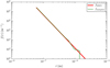 |
Fig. 1. Distribution functions of the MRN distribution and of our sample. |
The qth moment of this distribution can be calculated as
 (5)
(5)
The qth moment has the dimension [Length]q, so
 (6)
(6)
is a length scale. If the MRN distribution is replaced by a monodisperse distribution
 (7)
(7)
then this distribution has the same qth moment as the MRN distribution. Figure 2 shows a plot of the length scale Lq versus the index q. The quantitative details of this curve depend on the values of rmin and rmax adopted.
It should be noted that monodisperse grains with r = L1 have the average length, those with r = L2 the average cross-sectional area, and those with r = L3 have the average mass of the MRN distribution. In addition, for the special case of the MRN distribution (power exponent x = −3.5), L5 coincides with the geometric mean of the largest and smallest radius,  , since
 (8)
(8)
For the values shown in the present study, it is L5 = 0.354 μm.
2.3. Building clusters
The way clusters are built can influence collisional behavior. We therefore give a detailed explanation of our algorithm here. After sampling N radii from the MRN distribution, the list of these radii is sorted and the grains are placed in descending order. This is done to make sure that the largest grains can be placed. Without sorting the list it can happen that the small grains are placed in a way that does not leave any space for the large grains. The grain to which the next grain is attached and the direction along which the two grains are separated are picked randomly. It can happen that after placement there is an overlap with another grain, in which case the grain is deleted again and the process of picking a grain to attach the next one to will start over. Grains outside of a sphere of a predefined radius are also deleted to ensure an approximately spherical shape.
This algorithm is comparable to the one presented by Guesnet et al. (2019), with the difference that they implement an inactivation probability for grains that can no longer have a new neighbor grain attached to them, which leads to varying porosities. In our algorithm, the requested value of the filling factor ϕ can be enforced by defining the spherical shape that all the grains must have. It is also similar to the algorithm described by Ringl et al. (2012b), except they do not randomly pick the grains to attach the next ones to, but find the one with the smallest local filling factor.
The properties of all the clusters that we built are summarized in Table 1. The numbers N, ϕ, r, and R are not independent of each other. For the MRN distribution we required N to be 5000 and defined the radius R such that the clusters could be built in an acceptable time; this resulted in a cluster radius of around 4 μm and a filling factor of around 0.3. We then tried to keep ϕ and R close to the resulting value for all other clusters while varying N or r. We note that our clusters thus all have approximately the same total mass, radius, and filling factor (see Table 1); the only difference is the radius of the grains r, and consequently the number of grains.
Overview of the parameters of the clusters used in this work.
We also counted the number of contacts Nc in the clusters by comparing all possible combinations of grain distances to the sum of their respective radii. As Table 1 shows, it is approximately Nc = 1.5N. This is in rough agreement with Wada et al. (2011), who showed that the coordination number Z is around 4 for a cluster with filling factor 0.3. Since for large clusters, it is Nc = NZ/2, that study predicts Nc = 2N; however, since surface grains are less coordinated, our number of contacts is below 2N.
We produce the clusters and let them relax to ensure equilibrium. This means simulating the cluster with a friction force proportional to the grain velocity in order to quench any movement of the grains.
After relaxation we set up a collision by taking two randomly rotated copies of the cluster, separating them by translation and boosting them towards each other at velocity v/2. All simulations are performed with 3 million timesteps (Δt = 1 ps), amounting to a total simulated time of 3 μs. For every cluster type (size distribution) and velocity we perform ten collisions with different rotation angles to enable statistical evaluation. The results in the following section are averages over ten collisions. Figure 3 presents snapshots of a collision of two MRN clusters at a collision velocity of v = 15 ms−1, which is non-violent in the sense that we do not observe significant fragmentation. Figure 4 shows snapshots of a collision at v = 30 ms−1 that exhibits a considerably larger amount of fragmentation.
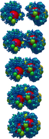 |
Fig. 3. Collision of the MRN clusters at v = 15 ms−1 with snapshots spaced by 0.1 μs. The grains are color-coded according to size. |
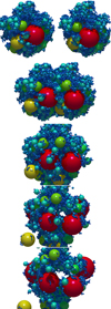 |
Fig. 4. Collision of the MRN clusters at v = 30 ms−1 with snapshots spaced by 0.15 μs. The grains are color-coded according to size. |
3. Results
3.1. Fragmentation
Kalweit & Drikakis (2006) defined a parameter Ns to measure fragmentation. We modify its definition slightly to adapt it to a polydisperse grain distribution as
 (9)
(9)
where the number of grains has been replaced by the total mass M of one cluster and masses M1 and M2 of the largest and second-largest fragments, respectively. The factor 2 in the denominator takes into account the fact that the collisions are performed with two identical clusters. In a collision which results in only one or two large fragments, the fraction (M1 + M2)/(2M) is close to 1 and Ns is 0. On the other hand, in a violent collision, which leaves many small fragments, the fraction approaches 0, and therefore Ns = 1. We use Ns as a measure of fragmentation. When the number of the fragments increases, so does the value of Ns.
A second quantity, X, measures the amount of sticking or agglomeration. Again adapting the original definition by Kalweit & Drikakis (2006) to polydisperse clusters, it is
 (10)
(10)
We follow the classification of Kalweit & Drikakis (2006) and Ringl et al. (2012a) that X > 0.15 identifies the sticking regime and X < 0.15 the fragmentation regime.
These properties can be measured by evaluating the simulation results with an algorithm for cluster analysis. We implemented the algorithm presented by Stoddard (1978) and used this code to identify all clusters in the last time step of the simulations.
Figures 5 and 6 show a plot of the agglomeration measure X and the fragmentation parameter Ns as a function of impact velocity for the mono- and polydisperse clusters, respectively. We make the following observations:
 |
Fig. 5. Panel a: agglomeration parameter X and panel b: fragmentation parameter Ns as a function of collision velocity v for a collection of radii of the monodisperse clusters. |
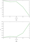 |
Fig. 6. Panel a: agglomeration parameter X and panel b: fragmentation parameter Ns as a function of collision velocity v for the MRN distribution. |
-
The clusters tend to show higher fragmentation for higher collision velocities. Higher velocities mean higher impact energy. Additional energy can be used to break more contacts between grains, and therefore enhance fragmentation.
-
Clusters that consist of larger grains show stronger fragmentation. The clusters with larger grains have fewer grains and fewer contacts. As shown in Sect. 2.1, the break-up energy of a contact grows as r, but the number of contacts in a cluster of given mass decreases as r−3. So for larger grain sizes, the total energy of all contacts is smaller and the cluster can be broken up more easily.
-
The plot of the fragmentation parameter Ns for the MRN distribution most closely resembles the monodisperse cluster of grain radius 0.314 μm or 6.28 rmin. This is the length scale found when calculating the 4.6th moment of the MRN distribution.
-
The plot of the agglomeration parameter X for the MRN distribution most closely resembles the monodisperse cluster of grain radius 0.353 μm or 7.06 rmin, which is the length scale associated with the 5.0th moment of the MRN distribution.
-
Monodisperse clusters with larger grains show higher fragmentation than those with smaller grains. This can be explained by the fact that the force of adhesion scales with the radius, while the mass of the grains grows as r3. This means that the adhesive forces can withstand higher grain accelerations without contacts breaking.
3.2. Energy dissipation
The kinetic energy remaining in the system can be calculated by measuring the kinetic translational and rotational energy of each grain and adding these up for all grains in a collision. We did this for all ten collisions of the same collision velocity and for each time step we took the average of the ten collisions. We note that the potential energy is at least a factor of 100 lower than the kinetic energy.
Figures 7a–b show the time evolution of the kinetic energy remaining in the clusters for a monodisperse cluster and the MRN cluster for several collision velocities; a grain radius r was selected where the time evolutions resemble each other closely. We observe that after roughly 0.5–1.0 μs, the energy stays nearly constant for most collisions. This time corresponds roughly to the passage time of the two clusters, 2R/v, since R = 4 μm and v = 10–30 m s−1. This also demonstrates that our simulation time of 3 μs is sufficient to capture all relevant aspects of the collision dynamics. The kinetic energy does not decay to zero for higher collision velocities because the debris of fragmented clusters will move away at undecelerated velocities.
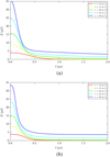 |
Fig. 7. Time evolution of the kinetic energy remaining in the cluster after the collision at time t = 0 for panel a: monodisperse granular clusters with grain radius r = 0.314 μm, and panel b: granular clusters with MRN grain size distribution. |
For other grain radii r the temporal distributions of the kinetic energy show considerable deviations from that of the MRN distribution. We document this feature by displaying the kinetic energy left in the collided clusters at the time of t = 0.5 μs (i.e., towards the end of the collision) in Fig. 8. This figure in particular documents that around the cluster size of r = 0.314 μm chosen in Fig. 7b, the energy dissipation does not depend strongly on the exact value of r; therefore, we do not show more examples of the time evolution of energy dissipation such as those provided in Fig. 7.
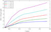 |
Fig. 8. Kinetic energies remaining in the monodisperse clusters at time t = 0.5 μs as a function of grain radius r. |
From Figs. 7 and 8 we observe the following:
-
For monodisperse clusters, the larger the grain radii, the more energy is left after the collision. The clusters with smaller grains break up less easily (see above) and have more grains and more contacts that can dissipate energy. Energy dissipation is more efficient in these cases.
-
The energy dissipation behavior of the MRN cluster is most similar to the monodisperse clusters with grain radii of 0.298–0.314 μm or (5.96–6.28) rmin. This length range corresponds to the 4.5th–4.6th moment of the MRN distribution.
-
Monodisperse clusters with smaller grains dissipate collision energies faster and to a higher extent than those with larger grains because, as above, for smaller grains adhesion is much more effective. In addition, these clusters consist of more grains so there are more grain contacts, which is where friction occurs.
3.3. Discussion
The fragmentation velocity can be defined as the velocity where the sticking parameter X decreases below 0.15 (Kalweit & Drikakis 2006; Ringl et al. 2012a). Figure 5 shows that this occurs at velocities of v = 27 (19, 12.5) m s−1 for grain radii of r = 0.396 (0.453, 0.57) μm. Previous results are available for r = 0.75 μm grain aggregates. Clusters with N = 7200 (filling factor 20.5%, radius R = 28 μm) have a fragmentation threshold of 17 m s−1 (Ringl et al. 2012a); given the difference in aggregate size, this is compatible with our present results. Gunkelmann et al. (2016) investigated the influence of aggregate porosity on the fragmentation velocity for clusters of size R = 30 μm, and found no sensitive effect; the fragmentation velocity decreases only for filling factors below around 12%. On the other hand, we observe fragmentation for higher energies than Dominik & Tielens (1997), Suyama et al. (2008), and Wada et al. (2008). This feature has been discussed extensively by Ringl et al. (2012a) who find that energy dissipation by friction during the collision (see Sect. 3.2) is responsible for this discrepancy.
As shown above in Sect. 3.1 and 3.2, MRN clusters behave similarly in terms of fragmentation and energy dissipation of monodisperse clusters if their size R is appropriately chosen. The moments of the distribution provide a suitable means to classify the appropriate size; we found that monodisperse radii adapted for q = 4.5–5.0 closely reproduce the results of the MRN distribution. The corresponding radius is about a factor of 6 larger than the smallest (and most probable) radius in the MRN distribution.
Ormel et al. (2009) discuss which radius of monodisperse grains r to choose such that monodisperse aggregates best represent the physical properties of MRN aggregates in size range [rmin, rmax]. When considering the mechanical strength of aggregates, they conclude that  . However, when focusing on aerodynamic properties (i.e., the ratio of cross section to mass) a two-dimensional analysis shows that
  ; in three dimensions, r is somewhat smaller. This latter result is in close agreement with our study that indicates that for collisional properties r should be taken as the geometric average of rmin and rmax.
4. Conclusions
In summary, we conclude that polydisperse clusters obeying the MRN size distribution can be replaced by clusters of monodisperse grains. In the case studied here, the appropriate grain size corresponds to the length scale provided by the geometric mean of the largest and smallest radius of the MRN distribution; it corresponds to the fifth moment of the polydisperse size distribution, which is about six times larger than the smallest (and most probable) radius in the MRN distribution. It is also larger than grains with the average size or even mass of the MRN distribution. The reason is that small grains enhance the energy dissipation and hinder fragmentation.
In future work attention should be given to the way clusters of polydisperse grains are built. The algorithm presented here has been optimized on building clusters with a pre-determined filling factor; it enforces contacts between large grains. In realistic clusters, large grains might be preferentially surrounded by small grains. It will be relevant to study the consequences of the cluster structure on fragmentation and energy dissipation.
Acknowledgments
We thank Cornelis P. Dullemond for fruitful discussions. Simulations were performed at the High Performance Cluster Elwetritsch (RHRK, TU Kaiserslautern, Germany).
References
- Birnstiel, T., Dullemond, C. P., & Brauer, F. 2010a, A&A, 513, A79 [NASA ADS] [CrossRef] [EDP Sciences] [Google Scholar]
- Birnstiel, T., Ricci, L., Trotta, F., et al. 2010b, A&A, 516, L14 [NASA ADS] [CrossRef] [EDP Sciences] [Google Scholar]
- Blum, J. 2010, Res. Astron. Astrophys., 10, 1199 [NASA ADS] [CrossRef] [Google Scholar]
- Blum, J., & Wurm, G. 2000, Icarus, 143, 138 [NASA ADS] [CrossRef] [Google Scholar]
- Dominik, C., & Tielens, A. G. G. M. 1997, ApJ, 480, 647 [NASA ADS] [CrossRef] [Google Scholar]
- Dominik, C., Blum, J., Cuzzi, J. N., & Wurm, G. 2007, in Protostars and Planets V, eds. B. Reipurth, D. Jewitt, & K. Keil (Tucson, AZ: Univ. Arizona Press), 783 [Google Scholar]
- Eggersdorfer, M. L., & Pratsinis, S. E. 2012, Aerosol Sci. Technol., 46, 347 [NASA ADS] [CrossRef] [Google Scholar]
- Ellerbroek, L. E., Gundlach, B., Landeck, A., et al. 2017, MNRAS, 469, S204 [CrossRef] [Google Scholar]
- Guesnet, E., Dendievel, R., Jauffres, D., Martin, C. L., & Yrieix, B. 2019, Phys. A: Stat. Mech. Appl., 513, 63 [CrossRef] [Google Scholar]
- Gunkelmann, N., Ringl, C., & Urbassek, H. M. 2016, A&A, 589, A30 [NASA ADS] [CrossRef] [EDP Sciences] [Google Scholar]
- Kalweit, M., & Drikakis, D. 2006, Phys. Rev. B, 74, 235415 [NASA ADS] [CrossRef] [Google Scholar]
- Katsuragi, H., & Blum, J. 2018, Phys. Rev. Lett., 121, 208001 [NASA ADS] [CrossRef] [Google Scholar]
- Kloss, C., Goniva, C., Hager, A., Amberger, S., & Pirker, S. 2012, Prog. Comput. Fluid Dyn., 12, 140 [Google Scholar]
- Mathis, J. S., Rumpl, W., & Nordsieck, K. H. 1977, ApJ, 217, 425 [NASA ADS] [CrossRef] [Google Scholar]
- Ormel, C. W., Paszun, D., Dominik, C., & Tielens, A. G. G. M. 2009, A&A, 502, 845 [NASA ADS] [CrossRef] [EDP Sciences] [Google Scholar]
- Petit, J. C., & Medina, E. 2018, Phys. Rev. E, 98, 022903 [NASA ADS] [CrossRef] [Google Scholar]
- Ringl, C., & Urbassek, H. M. 2012, Comput. Phys. Commun., 183, 986 [NASA ADS] [CrossRef] [Google Scholar]
- Ringl, C., Bringa, E. M., Bertoldi, D. S., & Urbassek, H. M. 2012a, ApJ, 752, 151 [NASA ADS] [CrossRef] [Google Scholar]
- Ringl, C., Bringa, E. M., & Urbassek, H. M. 2012b, Phys. Rev. E, 86, 061313 [NASA ADS] [CrossRef] [Google Scholar]
- Saw, E.-W., Salazar, J. P. L. C., Collins, L. R., & Shaw, R. A. 2012, New J. Phys., 14, 105030 [NASA ADS] [CrossRef] [Google Scholar]
- Schräpler, R., Blum, J., Seizinger, A., & Kley, W. 2012, A&A, 758, A35 [Google Scholar]
- Schräpler, R., Blum, J., Krijt, S., & Raabe, J.-H. 2018, ApJ, 853, 74 [NASA ADS] [CrossRef] [Google Scholar]
- Stoddard, S. D. 1978, J. Comput. Phys., 27, 291 [NASA ADS] [CrossRef] [Google Scholar]
- Suyama, T., Wada, K., & Tanaka, H. 2008, ApJ, 684, 1310 [NASA ADS] [CrossRef] [Google Scholar]
- Umstätter, P., Gunkelmann, N., Dullemond, C. P., & Urbassek, H. M. 2019, MNRAS, 483, 4938 [NASA ADS] [Google Scholar]
- Wada, K., Tanaka, H., Suyama, T., Kimura, H., & Yamamoto, T. 2008, ApJ, 677, 1296 [NASA ADS] [CrossRef] [Google Scholar]
- Wada, K., Tanaka, H., Suyama, T., Kimura, H., & Yamamoto, T. 2011, ApJ, 737, 36 [NASA ADS] [CrossRef] [Google Scholar]
- Whizin, A. D., Blum, J., & Colwell, J. E. 2017, ApJ, 836, 94 [NASA ADS] [CrossRef] [Google Scholar]
- Wurm, G., & Blum, J. 1998, Icarus, 132, 125 [NASA ADS] [CrossRef] [Google Scholar]
All Tables
All Figures
|
Fig. 1. Distribution functions of the MRN distribution and of our sample. |
| In the text | |
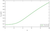 |
Fig. 2. Length scale Lq, Eq. (5), vs. the moment index q. |
| In the text | |
|
Fig. 3. Collision of the MRN clusters at v = 15 ms−1 with snapshots spaced by 0.1 μs. The grains are color-coded according to size. |
| In the text | |
|
Fig. 4. Collision of the MRN clusters at v = 30 ms−1 with snapshots spaced by 0.15 μs. The grains are color-coded according to size. |
| In the text | |
|
Fig. 5. Panel a: agglomeration parameter X and panel b: fragmentation parameter Ns as a function of collision velocity v for a collection of radii of the monodisperse clusters. |
| In the text | |
|
Fig. 6. Panel a: agglomeration parameter X and panel b: fragmentation parameter Ns as a function of collision velocity v for the MRN distribution. |
| In the text | |
|
Fig. 7. Time evolution of the kinetic energy remaining in the cluster after the collision at time t = 0 for panel a: monodisperse granular clusters with grain radius r = 0.314 μm, and panel b: granular clusters with MRN grain size distribution. |
| In the text | |
|
Fig. 8. Kinetic energies remaining in the monodisperse clusters at time t = 0.5 μs as a function of grain radius r. |
| In the text | |
Current usage metrics show cumulative count of Article Views (full-text article views including HTML views, PDF and ePub downloads, according to the available data) and Abstracts Views on Vision4Press platform.
Data correspond to usage on the plateform after 2015. The current usage metrics is available 48-96 hours after online publication and is updated daily on week days.
Initial download of the metrics may take a while.