| Issue |
A&A
Volume 631, November 2019
|
|
|---|---|---|
| Article Number | A152 | |
| Number of page(s) | 12 | |
| Section | Planets and planetary systems | |
| DOI | https://doi.org/10.1051/0004-6361/201936521 | |
| Published online | 13 November 2019 | |
Dusty phenomena in the vicinity of giant exoplanets
1
Space Research Institute (IWF), Austrian Academy of Sciences,
Schmiedlstrasse 6, 8042 Graz, Austria
e-mail: This email address is being protected from spambots. You need JavaScript enabled to view it.
2
Institute of Laser Physics, SB RAS,
Novosibirsk 630090, Russia
e-mail: This email address is being protected from spambots. You need JavaScript enabled to view it.
3
Institute of Physics, Karl-Franzens University of Graz, Universitätsplatz 5,
8010 Graz, Austria
e-mail: This email address is being protected from spambots. You need JavaScript enabled to view it.
Received:
19
August
2019
Accepted:
1
October
2019
Abstract
Context. Hitherto, searches for exoplanetary dust have focused on the tails of decaying rocky or approaching icy bodies only at short circumstellar distances. At the same time, dust has been detected in the upper atmospheric layers of hot jupiters, which are subject to intensive mass loss. The erosion and/or tidal decay of hypothetic moonlets might be another possible source of dust around giant gaseous exoplanets. Moreover, volcanic activity and exozodiacal dust background may additionally contribute to exoplanetary dusty environments.
Aims. In the present study, we look for photometric manifestations of dust around different kinds of exoplanets (mainly giants).
Methods. We used linear approximation of pre- and post-transit parts of the long-cadence transit light curves (TLCs) of 118 Kepler objects of interest after their preliminary whitening and phase-folding. We then determined the corresponding flux gradients G1 and G2, respectively. These gradients were defined before and after the transit border for two different time intervals: (a) from 0.03 to 0.16 days and (b) from 0.01 to 0.05 days, which correspond to the distant and adjoining regions near the transiting object, respectively. Statistical analysis of gradients G1 and G2 was used for detection of possible dust manifestation.
Results. It was found that gradients G1 and G2 in the distant region are clustered around zero, demonstrating the absence of artifacts generated during the light curve processing. However, in the adjoining region, 17 cases of hot jupiters show significantly negative gradients, G1, whereas the corresponding values of G2 remain around zero. The analysis of individual TLCs reveals the localized pre-transit decrease of flux, which systematically decreases G1. This effect was reproduced with the models using a stochastic obscuring precursor ahead of the planet.
Conclusions. Since only a few TLCs show the presence of such pre-transit anomalies with no analogous systematic effect in the post-transit phase, we conclude that the detected pre-transit obscuration is a real planet-related phenomenon. Such phenomena may be caused by dusty atmospheric outflows or background circumstellar dust compressed in front of the mass-losing exoplanet, the study of which requires dedicated physical modeling and numeric simulations. Of certain importance may be the retarding of exozodiacal dust relative to the planet by the Poynting-Robertson effect leading to dust accumulation in electrostatic or magnetic traps in front of the planet.
Key words: planets and satellites: general / interplanetary medium / zodiacal dust
© ESO 2019
1 Introduction
Exoplanetary environments are nowadays the focus of extensive theoretical modeling and dedicated observations, traditionally in spectral lines (Lammer & Khodachenko 2015). The available broadband photometry may provide additional valuable environmental information for significantly larger number of objects, as compared to those studied by spectral methods. At the same time, only the signatures of the dust component are detectable in such studies. Until now, the manifestations of dust have been noticed on decaying rocky planets in the form of tails (e.g., Brogi et al. 2012; Budaj 2013; Garai 2018; Sanchis-Ojeda et al. 2015). The presence of dust was also reported at altitudes of ~3000 km in gaseous giant exoplanets (Huitson et al. 2012; Wang & Dai 2019), and it is quite possible that such dust is dragged by the escaping planetary upper atmospheric material driven by stellar X-ray and ultraviolet (XUV) heating and tidal forces (Shaikhislamov et al. 2016). Among the sources of the dust at giant exoplanets could be the erosion of moonlets by meteoroids and plasma flows, tidal decay and evaporation of heated and liquified satellites, satellite volcanic activity, and magnetospheric capture of interplanetary (e.g., exozodiacal) dust (Spahn et al. 2019). The dust product of any of these processes can manifest itself as dusty obscuring matter (DOM), which transits over a stellar disk ahead of or behind the planet, generating tiny anomalies in the exoplanetary transit light curves (TLCs), especially before and after planetary eclipses.
In that respect, the TLCs provided by the space telescope Kepler represent promising but still superficially studied source of information on the pre/post-transit anomalies and the related manifestations of DOM. Hitherto, the out-of-transit parts of exoplanetary TLCs have only been studied for a cumulative search of exomoons and evaluation of particular candidates around Kepler-1625b (Teachey et al. 2018). Here we analyze for the first time the transit vicinities of many individual Kepler objects of interest (KOIs). The maximal duration of available data records and their highest precision make Kepler data the best choice to search for tenuous photometric effects of DOM.
The analysis presented here involves a specially elaborated method, which is explained in Sect. 2. The obtained results are described in Sect. 3 and conclusions are presented in Sect. 4.
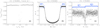 |
Fig. 1 Example of the light curve processing for the star KIC 5780885. Panel a: approximation of the transit background (open squares) with a sixth-order polynomial Fb (tk) (solid line); panel b: phase-folded TLC, ΔF(Δt), with near-transit border parts BP1 and BP2 indicated (blue boxes); panel c: clipped border parts (labeled) vs. the border distance δt ready for comparison. The black horizontal bar in (c) corresponds to the radius ingress (egress) time of the planet. |
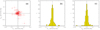 |
Fig. 2 Distributions of the pre-ingress, G1, and post-egress, G2, gradientestimates of TLC for the distant pre- and post-transit regions with τmin = 0.03 days and τmax = 0.16 days for 114 KOIs with errors < 0.05%∕day: panel a: G2 vs. G1 diagram; panel b: histogram of G1; panel c: histogram of G2. The value n is the number of estimates within a bin of histogram. |
2 Analysis method and stellar set
A natural way to detect DOM structures co-moving with the transiting object in broadband photometry is to search for flux variations a short time before the ingress of the planet on the stellar disk and after the egress. For this purpose we use the publicly available light curves from the Kepler mission (NASA Exoplanet Archive1) after Pre-search Data Conditioning (FPDC hereinafter), where instrumental drifts, focus changes, and thermal transients are removed or suppressed (Jenkins et al. 2010). Our survey uses the long-cadence data with photon accumulation (i.e., exposure) period of δtL = 29.4 min. This approach provides the highest precision of the input light curves, although it cannot resolve the details of the ingress and egress parts of the TLCs. The short-cadence data with the counting period of δtS = 1 min, in spite of higher time resolution, are available for a lesser number of stars and not for all quarters; and they also increase the detection threshold of DOM by a factor of 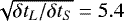 .
.
To remove the residual instrumental drifts as well as the stellar variability at timescales longer than the transit duration, after removal of the transit parts of duration Δttr plus the margins of ± 0.01 days, we approximate the normalized light curve FPDC(tk)∕⟨FPDC(tk)⟩, which covers the time interval ± 10Δttr centered at the particular transit, (see Fig. 1a), with a sixth-order polynomial  , where tk is the flux measurement time, a, b, c, d, e, f, g are the fitted coefficients, and ⟨FPDC(tk)⟩ is the average flux of the light curve. This approximation is an iterative process (10 iterations), with the consequent exclusion of remaining stellar flares and transit counts above the threshold |[FPDC(tk)∕⟨FPDC(tk)⟩] − Fb(tk)| > 3 σb, where σb is a standard deviation from the approximation Fb(tk). Since the final approximation Fb(tk) is insensitive to the transit (Fig. 1a), we use it as reference level to determine the flux decrease during the transit: ΔFk = [FPDC(tk)∕⟨FPDC(tk)⟩] − Fb(tk), which is used in further analysis.
This light curve “whitening” procedure enables us to finally obtain a phase-folded TLC ΔF(Δt) (Fig. 1b), where Δt = tk − tE is the time counted for each transit with number E = 0, 1, 2, … relative to its mid-time, tE = t0 + PtrE. The cumulative reference time t0 and the transit period Ptr are taken from the NASA Exoplanet Archive.
To detect the possible manifestation of DOM, which is supposedly concentrated around an exoplanet, the linear gradients G1,2 ≡ ∂(ΔF)∕∂(δt) were calculated in the time intervals − τmax < δt < −τmin and τmin < δt < τmax for the pre-ingress and post-egress parts of the TLCs, respectively. Here, δt = Δt ± 0.5Δttr is the border distance time counted from the transit border in folded TLC, calculated with the cumulative transit duration Δttr from the NASA Exoplanet Archive. The gradients G1 and G2 were found in two interval ranges: (a) in the adjoining pre/post-transit region, i.e., between τmin = 0.01 days (the half-exposure of the flux record) and τmax = 0.05 days; (b) in the distant region, that is, between τmin = 0.03 days and τmax = 0.16 days, which correspond approximately to the planetocentric distances from ~ 2 to ~ 17 planetary radii.
Altogether, a set of 118 KOIs with “confirmed” or “candidate” status in the NASA Exoplanet Archive was compiled. This set consists of selected objects from the lists in Aizawa et al. (2018), whose short-cadence light curves were used to search for exo-rings (i.e., specific structures of the dusty matter around planets). Since in our study we deal with the long-cadence data only, the set of corresponding long-cadence light curves of the objects from Aizawa et al. (2018) was extended with other high-quality light curves of objects from the NASA Exoplanet Archive with the nominated signal-to-noise ratio (S/N) ≳ 103 (i.e., the transit depth normalized by the mean uncertainty in the flux during the transits as it was published in the KOI cumulative table of the NASA Exoplanet Archive). For the selection of KOIs from the list in Aizawa et al. (2018), the same version of the S/N definition as that used in the NASA Exoplanet Archive was considered, but with a less conservative selection threshold of ≳ 100. In cases of multi-planet systems, the objects with maximal transit depth were taken (one per system). The total set of KOIs selected for our analysis is listed in Table C.1.
To visualize the possible DOM effects, the phase-folded TLC (Fig. 1b) is clipped according to Fig. 1c. The clipping consists in the combination of the near-transit border parts (BP1 and BP2 in Fig. 1b) of the folded TLC to simplify their comparison. The null-punkt of the abscissa scale in Fig. 1c δt = 0 corresponds to the time Δt ± 0.5Δttr of the borders of transit. In fact, the observable transit borders in long-cadence light curves are shifted from those, defined as above, on half exposure period, i.e., on δtL∕2, that is −0.01 and +0.01 days for the transit start- and end- times, respectively. Correspondingly, the clipped border parts of folded TLC show the sharp minimum in Fig. 1c.
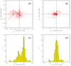 |
Fig. 3 Distributions of pre-ingress (G1) and post-egress (G2) gradients estimated in the adjoining regions (τmin = 0.01 and τmax = 0.05 days). Panel a: G2 vs. G1 diagram for90 KOIs with gradient errors (marked by bars) of less than 0.2%/day; panel b: diagram analogous to (a), but for all 114 KOIs considered; panel c: histogram of G1 for all estimates (i.e., all objects); panel d: histogram of G2 for all estimates (i.e., all objects). The value n is the number of estimates within a bin of a histogram. |
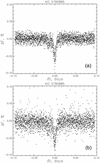 |
Fig. 4 Effect of imperfect approximation of the transit reference level Fb(tk) in the case of KIC 5780885 in Fig. 1c. Panel a: approximation with a sixth-order polynomial, commonly used in our study, which gives G1 = −0.26 ± 0.05 and G2 = 0.05 ± 0.05%/day; panel b: trial approximation with first-order polynomial covering the whole Ptr, which gives G1 = −0.32 ± 0.10 and G2 = 0.04 ± 0.11%/day. |
3 Results
First, we present the results obtained for the distant region with τmin = 0.03 days and τmax = 0.16 days (Fig. 2). One can see that most of the G1,2 estimate points cluster around G1 = G2 = 0. Several deviated estimates with G1 > 0 and G2 < 0 could be a manifestation of the forward-scattering by micron dust. Atmospheric aerosols could result in the increase of flux only by δ(ΔFk) = 32.5 ppm for ~1 μm particles (see Table 2 in García & Cabrera 2018) on the phase-angle scale 20o (Eq. (2) in DeVore et al. 2016), which corresponds to the timescale τs ~ (20o∕360o)Ptr for the transit period Ptr. Taking the typical Ptr ~ 10 days, one can estimate τs ~ 0.6 days and |G1,2|~ δ(ΔFk)∕τs < 0.005%∕day. This atmospheric aerosol contribution appears negligible in comparison with the obtained gradients |G1,2| > 0.05%∕day, which may however be not sufficiently reliable. For example, the TLC of Kepler-26b orbiting around KIC 9757613 shows the transits with maximal scattering-like gradients: G1 = 0.105 ± 0.040%∕day and G2 = −0.158 ± 0.047%∕day at 2.6 and 3.3 standard-error confidence level, respectively.
Another population of the deviating gradient estimates with G1 < 0 could be a manifestation of the large (≫1 μm) obscuring particles. However, the contribution of such negative gradient cases in the total G1 -distribution in Fig. 2b is insignificant. This is confirmed by an insignificant skewness, 0.35 ± 0.23, of the G1 -distribution (see Appendix A).
In summary, one can conclude that insignificant gradients G1,2 in the distant region correspond to the mainly dustless environments. This nondetection result can also be considered as a verification of the light curve processing method used, which does not generate any systematic errors or artifacts.
Closer to planets, that is, in the adjoining pre- and post-transit regions with τmin = 0.01 days and τmax = 0.05 days, the analogous G2 versus G1 diagram has a different appearance (Fig. 3). One can see the shift of many estimate points towards the negative G1 (Fig. 3a,b) as well as the bimodal character of the G1-histogram (Fig. 3c). There is also an undisturbed normal population of gradient estimates clustered around G1 = 0 (Fig. 3c) and G2 = 0 (Fig. 3d). Another population of gradient estimates with G1 < 0 and G2 ~ 0 (see Fig. 3d) might be related with the pre-transit manifestations of DOM; its existence is also confirmed by the significant skewness − 0.96 ± 0.23 of the G1 -distribution in Fig. 3c.
Theoretically, the known phenomenon of transit timing variations (TTVs), that is, the time-shifts of a TLC as a whole, could blur the transit borders in the folded TLC and create misleading gradients, namely G1 < 0 and G2 > 0. However, such shifts are known to oscillate in time around the linearly predicted ephemeride time of the transit tE (Holczer et al. 2016). Correspondingly, the TTV effect should blur both ingress and egress parts of the folded TLC. Hence, TTV cannot explain the observed just pre-transit flux drops without a detectable post-transit effect.
Anotherfactor that may affect a light curve is variation of the planetary phase (e.g., Esteves et al. 2015). However, variation of this kind gives negligible gradients Gph ~ 10−4Ap∕(0.5Ptr), where Ap ≤ 150 ppm is the planetary brightness amplitude (see Table 5-8 in Esteves et al. 2015), and the factor 10−4 is the transforming coefficient from ppm flux units into percent used here. Taking a typical transit period Ptr ~ 3 days for hot Jupiters, one can estimate that Gph ≲ 0.01%/day. Therefore, the second peak at G1 ≈ 0.3%/day in Fig. 3c cannot be attributed to planetary phase variability.
An imperfect polynomial approximation of the transit reference level Fb (tk) might hypothetically produce a misleading DOM-like effect. However, since the polynomial approximation is made for the sufficiently long part of the light curve (±10 Δttr around the mid of transit) without account of the transit itself (i.e., with the removed transit), the planetary circumference would not significantly affect this approximation. We simulated the effects of imperfect definition of Fb (tk) using its linear approximation instead of a sixth-order polynomial. The result was an increased dispersion of ΔF before and after the folded TLC without a noticeable systematic effect on G1 or G2 (see Fig. 4).
Figure 5d shows that significantly (above three standard errors) negative values of G1 are clearly associated with the Jupiter-typeplanets with radii 10 ≲ Rp ≲ 25 (i.e., 1.0 ≲ log(Rp) ≲ 1.4) in units of the Earth radius. Since our data set includes the transits of objects sized up to ≈ 0.1 Jovian radii, the appearance of a pronounced negative G1 feature by the Jupiter-type and larger objects is not a selection effect (compare Figs. 5a and d). According to Fig. 5e, the significantly negative gradients G1 were found exclusively by hot Jupiters at extremely short orbits with radii 0.026 ≲ aorb ≲ 0.065 au, although the analyzed sample includes a wide range of objects with orbital distances of up to 1 au. A summary of the individual parameters of 17 KOIs, showing the most significant values of G1, is given in Table 1. This may indicate that the large size and short orbital distance of a planet are prerequisites of detectable DOM signatures. Moreover, the intensive material escape and mass-loss typical for the close-orbit hot jupiters might affect the evolution and distribution of the obscuring DOM. We note that no significant (beyond three standard errors) deviations of |G2| from zero were found among the considered objects (Figs. 5g–i), meaning the absence of any measurement and/or calculation artifacts in the performed analysis. Therefore, the negative deviations of G1 detected in the adjoining regions of a significant group of the studied objects appear to be real phenomena.
In Table 1 we also present estimations of the effective area obscured by DOM on the stellar disk as  for the case of G1 defined in the adjoining pre-transit region. Here the coefficient 0.01 adopts the gradient, G1, values, expressed in units of percent/day; the minus reflects the increase of the DOM particle concentration towards the planet; τmax = 0.05 days; and R* is the stellar radius from the NASA Exoplanet Archive. The estimated effective DOM area expressed in percent of the planetary cross-section varies in the considered set of objects from the minimal value of 0.4% achieved for KOI 1.01, up to the maximal value of 3.3% for KOI 203.01.
The average value ⟨SDOM⟩ = 4.8 × 10⁸ km2 corresponds to the dust cloud of N ≈ SDOM∕(QA) ~ 2.8 × 1024 grains with the typical diameter d ~ 10 μm (like in the Solar System zodiacal cloud) and the geometrical cross-section  . Here, Q = 2.19 is the extinction efficiency, that is, the ratio of the shadow cross-section of the particle and its geometrical cross-section A, which is calculated for a transparent sphere with the refractive index of 1.5 and the average wavelength of the Kepler photometry λ = 0.66 μm using the Mie scattering theory2.
The integral volume of all these dust grains is  . It is in fact very small, as compared to the scales of potential dust sources; for example the Solar-System-like zodiacal cloud with an integral volume of its dust particles ~1.4 × 10⁴ km3, which is equivalent to a 15 km-sized asteroid (Mennesson et al. 2019); a Jupiter-type KOI (~ 1.4 × 10¹⁵ km3) or its Io-like moon (~2.5 × 10¹⁰ km3). Altogether, the amount of dust estimated above, needed for the detected DOM manifestations, seems to be achievable with such orders-of-magnitude-larger sources.
Figure 6 shows the examples of the DOM-related features visible as an occasional decrease (arrowed) of radiation flux ΔF in the folded TLCs clustered in a narrow (≈0.01 day) range of pre-ingress time δt. There is a tendency for such features to repeat with the flux counting period 0.02 days (the best pronounced is the case of KIC 9941662). Apparently, this is a result of artificial clustering of flux measurements at mid-exposure times.
The most manifested DOM-related feature in the TLC of KIC 10619192 (Fig. 6a) was studied in detail as a typical case. Figure 7 shows the difference between the pre-ingress and post-egress parts of the folded TLC. One can see that the arrowed DOM-related feature is unique over the whole transit period. This means that this effect is really associated with the transiting object and its co-moving DOM structure, and is therefore unlikely to be an artifact.
We tried to simulate the DOM phenomenology assuming a hypothetic obscuring precursor (Fig. 8d) before the real planet (see also Appendix B). This precursor imitates a dust cloud ahead of the planet at a distance of five planetary radii. Since the same flux drop could be obtained with very different geometries and transparency of dust cloud, the equivalent opaque circular disk of the precursor was assumed for simplicity in the simulation.
Using the pixel-by-pixel integration over the stellar disk as in Fig. 8d, we achieved a certain resemblance between the modeled and real phase-folded TLCs (Figs. 8a,b) including the clustering effect (Fig. 8c). It is worth noting that the model parameters used in this simulation were neither fitted nor optimized to obtain an evident DOM-type effect. Only a rough empirical selection of parameters was done to find an appropriate scenario. An interesting feature consists in the fact that the synthetic TLC with the most similar behavior to observations was obtained in the simulations with a precursor that is stochastic in character. Specifically, the radius of the precursor was randomly taken in the range between zero and 0.5 Rp, whereas its appearance time was randomized in the range [0; 375 days] with an average time interval of 0.0375 days between individual DOM events. The duration of each DOM event was 0.02 days (i.e., the exposure time) with a constant area of eclipsing DOM for each individual event. The specific planetary and stellar parameters used in the simulation were taken for the object KIC 10619192 from the NASA Exoplanet Archive. Altogether, the model realistically reproduces the stochastic variability of flux decrease within the pre-transit time interval − 0.02 < δt < −0.01 days, related to the investigated DOM effect (see Fig. 9).
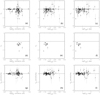 |
Fig. 5 Gradients G1 and G2, measured in the adjoining regions, versus planetary parameters: radius Rp of planet in (a), (d), and (g); radius aorb of orbit in (b), (e), and (h); and the orbital period Ptr in (c),(f), and (i). The plots (a)–(c) and (g)–(i) show all the studied objects (squares with error bars) from Table C.1, while the middle row panels (d)–(f) present only significant (above three standard errors) deviations of |G1 | from zero (listed in Table 1). |
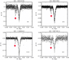 |
Fig. 6 Examples of DOM manifestations (arrowed) in the pre-ingress parts of folded and clipped TLCs (pluses), showing significant values of gradient G1. The horizontal bars correspond to the radii of considered planets, i.e., ingress-time. |
Objects with a significant manifestation of pre-transit DOM.
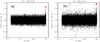 |
Fig. 7 Visualization of the pre-transit DOM manifestation (arrowed) in the light curve of KIC 10619192 above the background of cleared (panel a) and noncleared (panel b) folded out-of-transit parts (Ptr − Δttr) of the light curve, i.e., during the whole transit period except for the transit itself. |
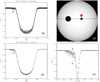 |
Fig. 8 Modeling of the pre-transit DOM manifestations (arrowed) in the case of KIC 10619192. Panel a: real folded TLC; panel b: synthetic folded TLC; panel c: clipped TLC to visualize the synthetic DOM effect like in Fig. 5; panel d: model geometry with the real planet, crossing the stellar disk along the solid line together with an idealized DOM precursor (arrowed). |
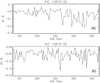 |
Fig. 9 Temporal variability of DOM effect as a pre-transit flux drop, measured at − 0.02 < δt < −0.01 days. Panel a: extraction from the real light curve of KIC 10619192; panel b: analogous plot for synthetic light curve based on the used model. The abscissa scale is in differential barycentric Julian days ΔJD, counted from the reference day 2454833.0. |
4 Conclusions
Below we summarize the major points, which may be concluded from the performed analysis and detections made.
- 1.
The absence of systematic deviation of the out-of-transit gradients G1 and G2 from zero in the distant regions (0.03 < |δt| < 0.16 days), and the same in the adjoining post-transit region (0.01 < δt < 0.05 days), but only for G2, means that there are no detectable DOM manifestations far from exoplanets, and in the closer regions behind them. This assures also the absence of influential artifacts from photometry or light curve processing.
- 2.
Since the discovered significant photometrical peculiarities (irregular drops of stellar radiation flux) take place only before the ingress (Figs. 3 and 4) in close vicinity of the transit border (Figs. 5 and 6) of only short-period giant exoplanets, and this effect was not pointed out in previous studies, we deal here with a hitherto unknown exoplanetary phenomenon. It appears to be a new aspect of hot Jupiter nature requiring investigation.
- 3.
The entirely pre-transit location of the found peculiarities excludes the possibility that these are photometric or processing artifacts (as explained in Sect. 3) or the manifestation of orbiting bodies (exomoons, moonlets, exo-rings, etc.) as a source of obscuring matter.
- 4.
The obtained results inspire the modeling work to simulate dusty atmospheric outflows (suggested in e.g., Wang & Dai 2019), which interact with the stellar winds, being compressed in front of the material-losing exoplanets (like in Shaikhislamov et al. 2016; Dwivedi et al. 2019). An alternative scenario could involve the retarding of exozodiacal dust relative to the planet by the Poynting-Robertson effect leading to dust accumulation in an electrostatic, magnetic, or dynamic trap before the planet. These scenarios require a dedicated modeling which will be the subject of future work.
Acknowledgements
The authors acknowledge the projects I2939-N27 and S11606-N16 of the Austrian Science Fund (FWF) for the support. M.L.K. is grateful also for the grant No. 18-12-00080 of the Russian Science Foundation.
Appendix A Skewness of G1,2 distributions
To characterize the asymmetry of a distribution, we calculated the sample skewness (Joanes & Gill 1998) of the obtained estimates of gradients G1,2
![Mathematical equation: \begin{equation*} S_{1,2} = \frac{\sqrt{n(n-1)}}{n-2} \left \{ \frac{\frac{1}{n} \sum_{i=1}^{n} (G_{1,2}^{i} - \langle G_{1,2} \rangle){}^{3}}{\left [\frac{1}{n} \sum_{i=1}^{n} (G_{1,2}^{i} - \langle G_{1,2} \rangle){}^{2} \right]^{3/2}} \right \}, \end{equation*}](/articles/aa/full_html/2019/11/aa36521-19/aa36521-19-eq6.png) (A.1)
(A.1)
where:  is the estimate of G1,2 for an individual KOI with a number i; n is the total number of considered objects; ⟨G1,2⟩ is the average value over all estimates
  . For the normal distribution the sample skewness has an expected value S1,2 = 0 and the variance
 ![Mathematical equation: $\sigma_{G}^{2}=6n(n-1)/[(n-2)(n+1)(n+3)]$](/articles/aa/full_html/2019/11/aa36521-19/aa36521-19-eq9.png) (Kendall & Stuart 1969).
(Kendall & Stuart 1969).
Appendix B Modeling of DOM effect in a TLC
Since various shapes and transparencies of a transiting dust cloud are possible, a universal method of pixel-by-pixel integration (Juvan et al. 2018) suitable for any shape of transiting object is applied to compute the corresponding TLCs. The dimming of stellar flux during transit is characterized by the part of starlight blocked by the transiting object
 (B.1)
(B.1)
where the coordinate system co-centered with the stellar disk with x-axis parallel to the planet orbit projection on the stellar disk is used; Is is radiation intensity at a given position (x,y) on the visible stellar disk, and I is the same intensity but disturbed by the transiter. The above-mentioned integrals can be replaced by sums over Np pixels with serial number i in the identical sets:
 (B.2)
(B.2)
The stellar limb darkening is taken into account according to the best (four coefficients) approximation by Claret & Bloemen (2011), depending on particular stellar effective temperature and gravity, adopted from the NASA Exoplanet Archive. The planetary data (radius Rp, semi-major axis aorb of the orbit, impact parameter β, mid-time t0 of the first observed transit, transit period Ptr) are also taken from the NASA Exoplanet Archive.
In the used reference system, the center exoplanetary shadow has coordinates
![Mathematical equation: \begin{equation*} x_{p} = a_{\textrm{orb}} \sin \left [\frac{2 \pi}{P_{\textrm{tr}}} (t_{k} - t_{0})\right], \end{equation*}](/articles/aa/full_html/2019/11/aa36521-19/aa36521-19-eq12.png) (B.3)
(B.3)
 (B.4)
(B.4)
where Rs is the stellar radius from the NASA Exoplanet Archive. The DOM is imitated by an opaque equivalent disk (see explanation in Sect. 3) at xDOM = xp + d and yDOM = yp. Here parameter d = 5Rp is a constant effective distance selected empirically but without a detailed fitting. The time step for ΔF calculation is adopted as τs = 0.00204 days. The next procedure consists in the smoothing of the obtained synthetic light curve with time step 10τs which reproduces the real effect of the long-cadence integration time 0.0204 days. Consequently, the smoothing reproduces a certain widening of the long-cadence TLC, manifested as sharp out-of-transit minima (synthesized in Fig. 8c) at 0 < |δt| < 0.01 days as seen in Figs. 1c and 6 for real TLCs. Moreover, the association of flux counts with the medial times of long-cadence exposures generates the 0.02-days periodicity in TLC, as for example in the case of KIC 9941662 in Fig. 6. We note that the synthetic light curves are treated further with the same processing pipeline as the real light curves.
Appendix C Supplementary material
Analyzed target set and processing results.
References
- Aizawa, M., Masuda, K., Kawahara, H., & Suto, Y. 2018, AJ, 155, 2018 [Google Scholar]
- Brogi, M., Keller, C. U., de Juan Ovelar, M., et al. 2012, A&A, 545, L5 [NASA ADS] [CrossRef] [EDP Sciences] [Google Scholar]
- Budaj J. 2013, A&A, 557, A72 [NASA ADS] [CrossRef] [EDP Sciences] [Google Scholar]
- Claret, A., & Bloemen, S. 2011, A&A, 529, A75 [NASA ADS] [CrossRef] [EDP Sciences] [Google Scholar]
- DeVore, J., Rappaport, S., Sanchis-Ojeda, R., Hoffman, K., & Rowe, J. 2016, MNRAS, 461, 2453 [NASA ADS] [CrossRef] [Google Scholar]
- Dwivedi, N. K., Khodachenko, M. L., Shaikhislamov, I. F., et al. 2019, MNRAS, 487, 4208 [NASA ADS] [CrossRef] [Google Scholar]
- Esteves, L. J., De Mooij, E. J. W., & Jayawardhana, R. 2015, ApJ, 804, 150 [NASA ADS] [CrossRef] [Google Scholar]
- Garai, Z. 2018, A&A, 611, A63 [NASA ADS] [CrossRef] [EDP Sciences] [Google Scholar]
- García, M. A., & Cabrera, J. 2018, MNRAS, 473, 1801 [NASA ADS] [CrossRef] [Google Scholar]
- Holczer, T., Mazeh, T., Nachmani, G., et al. 2016, ApJS, 225, 9 [NASA ADS] [CrossRef] [Google Scholar]
- Huitson, C. M., Sing, D. K., Vidal-Madjar, A., et al. 2012, MNRAS, 422, 2477 [NASA ADS] [CrossRef] [Google Scholar]
- Jenkins, J. M., Douglas, A. C., Chandrasekaran, H., et al. 2010, ApJ, 713, L87 [NASA ADS] [CrossRef] [Google Scholar]
- Joanes, D. N., & Gill, C. A. 1998, The Statistician, 47, 183 [Google Scholar]
- Juvan, I. G., Lendl, M., Cubillos, P. E., et al. 2018, A&A, 610, A15 [NASA ADS] [CrossRef] [EDP Sciences] [Google Scholar]
- Kendall, M. G., & Stuart, A. 1969, The Advanced Theory of Statistics (Houston: Griffin), 1 [Google Scholar]
- Lammer, H., & Khodachenko, M. 2015, Characterizing Stellar and Exoplanetary Environments (Heidelberg: Springer), 2015 [Google Scholar]
- Mennesson, B., Kennedy, G., Ertel, S., et al. 2019, BASS, 51, 324 [Google Scholar]
- Sanchis-Ojeda, R., Rappaport, S., Pallè, E., et al. 2015, ApJ, 812, 112 [NASA ADS] [CrossRef] [Google Scholar]
- Shaikhislamov, I. F., Khodachenko, M. L., Lammer, H., et al. 2016, ApJ, 832, 173 [NASA ADS] [CrossRef] [Google Scholar]
- Shaikhislamov, I. F., Khodachenko, M. L., Lammer, H., et al. 2018, MNRAS, 481, 5315 [NASA ADS] [CrossRef] [Google Scholar]
- Spahn, F., Sachse, M., Seiß, M., et al. 2019, Space Sci. Rev., 215, 11 [NASA ADS] [CrossRef] [Google Scholar]
- Teachey, A., Kipping, D. M., & Schmitt, A. R. 2018, AJ, 155, 36 [NASA ADS] [CrossRef] [Google Scholar]
- Wang, L., & Dai, F. 2019, ApJ, 873, L1 [NASA ADS] [CrossRef] [Google Scholar]
All Tables
All Figures
|
Fig. 1 Example of the light curve processing for the star KIC 5780885. Panel a: approximation of the transit background (open squares) with a sixth-order polynomial Fb (tk) (solid line); panel b: phase-folded TLC, ΔF(Δt), with near-transit border parts BP1 and BP2 indicated (blue boxes); panel c: clipped border parts (labeled) vs. the border distance δt ready for comparison. The black horizontal bar in (c) corresponds to the radius ingress (egress) time of the planet. |
| In the text | |
|
Fig. 2 Distributions of the pre-ingress, G1, and post-egress, G2, gradientestimates of TLC for the distant pre- and post-transit regions with τmin = 0.03 days and τmax = 0.16 days for 114 KOIs with errors < 0.05%∕day: panel a: G2 vs. G1 diagram; panel b: histogram of G1; panel c: histogram of G2. The value n is the number of estimates within a bin of histogram. |
| In the text | |
|
Fig. 3 Distributions of pre-ingress (G1) and post-egress (G2) gradients estimated in the adjoining regions (τmin = 0.01 and τmax = 0.05 days). Panel a: G2 vs. G1 diagram for90 KOIs with gradient errors (marked by bars) of less than 0.2%/day; panel b: diagram analogous to (a), but for all 114 KOIs considered; panel c: histogram of G1 for all estimates (i.e., all objects); panel d: histogram of G2 for all estimates (i.e., all objects). The value n is the number of estimates within a bin of a histogram. |
| In the text | |
|
Fig. 4 Effect of imperfect approximation of the transit reference level Fb(tk) in the case of KIC 5780885 in Fig. 1c. Panel a: approximation with a sixth-order polynomial, commonly used in our study, which gives G1 = −0.26 ± 0.05 and G2 = 0.05 ± 0.05%/day; panel b: trial approximation with first-order polynomial covering the whole Ptr, which gives G1 = −0.32 ± 0.10 and G2 = 0.04 ± 0.11%/day. |
| In the text | |
|
Fig. 5 Gradients G1 and G2, measured in the adjoining regions, versus planetary parameters: radius Rp of planet in (a), (d), and (g); radius aorb of orbit in (b), (e), and (h); and the orbital period Ptr in (c),(f), and (i). The plots (a)–(c) and (g)–(i) show all the studied objects (squares with error bars) from Table C.1, while the middle row panels (d)–(f) present only significant (above three standard errors) deviations of |G1 | from zero (listed in Table 1). |
| In the text | |
|
Fig. 6 Examples of DOM manifestations (arrowed) in the pre-ingress parts of folded and clipped TLCs (pluses), showing significant values of gradient G1. The horizontal bars correspond to the radii of considered planets, i.e., ingress-time. |
| In the text | |
|
Fig. 7 Visualization of the pre-transit DOM manifestation (arrowed) in the light curve of KIC 10619192 above the background of cleared (panel a) and noncleared (panel b) folded out-of-transit parts (Ptr − Δttr) of the light curve, i.e., during the whole transit period except for the transit itself. |
| In the text | |
|
Fig. 8 Modeling of the pre-transit DOM manifestations (arrowed) in the case of KIC 10619192. Panel a: real folded TLC; panel b: synthetic folded TLC; panel c: clipped TLC to visualize the synthetic DOM effect like in Fig. 5; panel d: model geometry with the real planet, crossing the stellar disk along the solid line together with an idealized DOM precursor (arrowed). |
| In the text | |
|
Fig. 9 Temporal variability of DOM effect as a pre-transit flux drop, measured at − 0.02 < δt < −0.01 days. Panel a: extraction from the real light curve of KIC 10619192; panel b: analogous plot for synthetic light curve based on the used model. The abscissa scale is in differential barycentric Julian days ΔJD, counted from the reference day 2454833.0. |
| In the text | |
Current usage metrics show cumulative count of Article Views (full-text article views including HTML views, PDF and ePub downloads, according to the available data) and Abstracts Views on Vision4Press platform.
Data correspond to usage on the plateform after 2015. The current usage metrics is available 48-96 hours after online publication and is updated daily on week days.
Initial download of the metrics may take a while.