| Issue |
A&A
Volume 631, November 2019
|
|
|---|---|---|
| Article Number | A17 | |
| Number of page(s) | 11 | |
| Section | The Sun | |
| DOI | https://doi.org/10.1051/0004-6361/201935967 | |
| Published online | 11 October 2019 | |
Revisiting the coronal current sheet model: Parameter range analysis and comparison with the potential field model
ReSoLVE Centre of Excellence, Space Climate Research Unit, University of Oulu, Oulu, Finland
e-mail: This email address is being protected from spambots. You need JavaScript enabled to view it.
Received:
27
May
2019
Accepted:
29
August
2019
Abstract
Aims. We study the properties of the coronal magnetic field according to the current sheet source surface (CSSS) model in 1976–2017 for all physically reasonable values of the three model parameters (cusp surface radius Rcs, source surface radius Rss, and current parameter a), and compare the CSSS field with the potential field source surface (PFSS) model field.
Methods. We used the synoptic maps of the photospheric magnetic field from the Wilcox Solar Observatory (WSO), National Solar Observatory/Kitt Peak (NSO/KP), and the NSO Synoptic Optical Long-term Investigations of the Sun Vector Spectromagnetograph (SOLIS/VSM) in order to calculate the coronal magnetic field according to the CSSS and PFSS models. We calculated the coronal field strength, its latitudinal variation and neutral line location, as well as its polarity match with the heliospheric magnetic field.
Results. The CSSS model can correct the erroneous latitudinal variation of the PFSS model if the source surface is sufficiently far out with respect to the cusp surface (Rss ≥ 3 ⋅ Rcs). The topology of the neutral line only slightly depends on source surface radius or current parameter, but excludes very low values of the cusp surface (Rcs ≤ 1.5). A comparison of the polarities gives an optimum cusp surface radius that varies in time between 2 and 5; a stronger current yields a larger optimum Rcs. Interestingly, the optimum polarity match percentages and optimum radii vary very similarly in the two models over the four solar cycles we studied.
Conclusions. The CSSS model can produce a stronger total coronal flux than the PFSS model and correct its latitudinal variation. However, the topology of the CSSS model is rather independent of horizontal currents and remains very similar to that of the PFSS model. Therefore, the CSSS model cannot improve the match of field polarities between corona and heliosphere.
Key words: Sun: corona / Sun: magnetic fields
© ESO 2019
1. Introduction
The coronal magnetic field is the source of the heliospheric magnetic field (HMF). Owing to the low density of the coronal plasma, the coronal magnetic field is difficult to measure consistently over long periods of time. However, it is possible to reconstruct the coronal field using photospheric measurements and coronal models. Magnetohydrodynamic (MHD) models are currently among the most sophisticated coronal models. They give a self-consistent solution to the full set of MHD equations that describe the coronal plasma and its magnetic field (e.g. Riley et al. 2006). However, MHD models are computationally demanding.
Magnetohydrostatic (MHS) models aim to solve the MHS equations, which describe the balance between the Lorentz force, plasma pressure, and gravitational force. There are no large-scale plasma flows, and the system can be considered stationary, that is, the system evolves macroscopically only over timescales that are long enough. In a general form the MHS equations are non-linear, which makes them difficult to solve analytically in three dimensions. One way to simplify the MHS equations is to restrict the coronal electric currents, so that there is only a field-aligned current and a current perpendicular to gravity (Low 1991). One formulation for this choice can be written as follows (Mackay & Yeates 2012):
 (1)
(1)
Here J is the total electric current density, B is the magnetic field, r is distance from the centre in spherical coordinates, and α and a are free parameters that quantify the twist of the magnetic field and the radial length scale of coronal currents, respectively. The first part of the current denotes the force-free field-aligned current, and the second part denotes the current that is perpendicular to gravity.
Bogdan & Low (1986) derived a set of solutions for the MHS equations that only include the currents perpendicular to gravity (α = 0). Neukirch (1995) used a somewhat similar approach, but also included the field-aligned currents with constant α. The class of models that have a = 0 and α ≠ 0 are non-linear force-free (NLFF) models, and have only the field-aligned current. The parameter α is generally non-zero and a function of position, but constant along magnetic field lines. Solving NLFF models on a global scale is mathematically quite challenging (see, e.g. Wiegelmann 2007; Contopoulos et al. 2011; Yeates et al. 2018). These models typically use the observed twist of the magnetic field as input, which requires data from vector magnetograms.
If α = a = 0, that is, when the corona does not include electrical currents, we obtain a potential solution for the magnetic field. One of the simplest and most widely used potential models is the potential field source surface (PFSS) model (Altschuler & Newkirk 1969; Schatten et al. 1969). It has been used, for example, to predict the solar wind speed (Wang & Sheeley 1997; Riley et al. 2015). The PFSS model assumes that there are no currents between the photosphere and a chosen distance rss in the corona, called the source surface. On the source surface the field lines are assumed to become radial, and plasma starts to dominate the magnetic field. The PFSS model can reproduce the large-scale sector structure of the HMF fairly well (Riley et al. 2006; Koskela et al. 2017). However, because the PFSS model does not include electric currents, it includes a systematic gradient in the radial field component that reaches zero at the neutral line (NL). This is contradictory to Ulysses observations, which show that there is no latitudinal gradient in the HMF radial component (Smith & Balogh 1995).
There are several modified versions of the PFSS model. Schatten (1972) presented a current sheet model, in which the coronal field is calculated using the PFSS model up to the source surface distance, where then the sign of the negative (inward) magnetic field lines is switched, so that the field points outwards everywhere at the source surface. A new set of harmonic coefficients is calculated for the unipolar outward-directed field at the source surface. Last, the orientation of field lines that were switched in the earlier step is restored. This non-zero field creates current sheets between areas of oppositely directed field regions. This model is sometimes called the potential field – current sheet (PFCS) model. The PFCS model produces the high-latitude field lines of the Pneuman & Kopp (1970) MHD solution better than the PFSS solution. However, the PFSS model performs better with low-latitude closed field lines (see Fig. 6 in Schatten 1972).
Zhao & Hoeksema (1992) derived the horizontal current source surface (HCSS) model, which uses the spherical source surface, but instead of a potential field, it uses the Bogdan & Low (1986) solution that includes horizontal electric currents. It produces a magnetic field configuration comparable with the PFSS model. Zhao & Hoeksema (1994) presented a model with the Bogdan & Low (1986) MHS solution, with a cusp surface (at the cusp points of coronal helmet streamers) and the Schatten (1972) reversal technique. This model is called horizontal current – current sheet (HCCS) model. The open high-latitude field lines match the PFCS model well, and the low-latitude, low-altitude closed field lines match the PFSS model.
The current sheet source surface (CSSS) model (Zhao & Hoeksema 1995) is a combination of the MHS solution by Bogdan & Low (1986) and the current sheet model by Schatten (1972). It includes both the cusp surface at the cusp points of the helmet streamers and the source surface at the Alfvén layer. At the cusp surface the magnetic field becomes open, and at the source surface the field becomes radial as the plasma starts to dominate the magnetic field. The CSSS model has three free parameters: cusp surface distance Rcs, source surface distance Rss, and the parameter a that describes the radial scale of horizontal currents (see Fig. 1). The equations for the CSSS model are derived in Sect. 2.
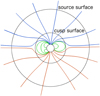 |
Fig. 1. Sketch of the CSSS model. The inner black circle is the photosphere, the middle circle is the cusp surface, and the outer circle is the source surface. At the cusp surface the field lines become open and at the source surface they become radial. The field lines that remain beneath the cusp surface are closed field lines. Red lines denote away-field, blue lines towards-field, and green lines are closed. |
Zhao & Hoeksema (1995) compared the magnitude of the radial field in the CSSS by varying Rcs between 1.6 and 2.25, Rss between 2.5 and 3.25, and a between 0 and 0.2 (all in units of the solar radius, Rs). Schüssler & Baumann (2006) showed that the CSSS model with Rcs = 1.7 and Rss = 10 can reproduce the time evolution of the open flux observed at 1 AU and report a latitude profile of the radial magnetic field that is consistent with Ulysses findings. Poduval & Zhao (2014) compared the PFSS and CSSS models in their ability to predict the solar wind speed using the flux tube expansion correlation by Wang & Sheeley (1990). They found that the CSSS model is able to predict the solar wind speed at 1 AU more accurately than the PFSS model, but the accuracy of this prediction varies within the solar cycle; the least accurate prediction is found at solar minimum. They therefore suggested that the free parameters of the model should be optimized separately for the different phases of the solar cycle. Poduval (2016) reported a similar comparison. She concentrated on the different phases of solar cycle 23 and the early part of cycle 24. She showed that even with constant parameters, the CSSS model can better predict the temporal variation of the solar wind speed over the different solar cycle phases than the PFSS model. The author also found that the latitudinal excursion of the heliospheric current sheet (HCS) is larger with the CSSS than with the PFSS model.
We here study the dependence of the CSSS model of the coronal field on the three model parameters (Rcs, Rss, and a) and the limitation imposed by different observations on the range of possible parameter values. We also compare the results of the CSSS model with the PFSS model. The paper is organized as follows. In Sect. 2 we discuss our data sources and introduce our methods. In Sect. 3 we present the CSSS model. In Sect. 4 we compare the field line configuration of the CSSS model with that of the PFSS model, in Sect. 5 we study the latitude gradient of the magnetic field, and in Sect. 6 we calculate the total open flux for different sets of CSSS model parameters. In Sect. 7 we study the topology of the field by calculating the NL location, and in Sect. 8 we investigate the polarity match between the coronal field and HMF. In Sect. 9 we discuss the obtained results and present our conclusions.
2. Data and methods
The heliospheric parameters (solar wind speed and HMF) were retrieved from the NASA/NSSDC OMNI 2 dataset. We used the hourly OMNI 2 data, which we smoothed with a 25-h running mean in order to remove short-term fluctuations. We required at least 7 h of data for each 25-h running mean window, otherwise the hour was neglected. According to Lockwood et al. (2006), the averaging length should be chosen so that the small-scale structures originating during heliospheric propagation are averaged out but the actual large-scale structure is not. We found that an averaging period of about one day was a good compromise. The window of 25 h corresponds to 13.2° in Carrington longitude.
We used synoptic maps of the photospheric magnetic field from the Wilcox Solar Observatory (WSO), the National Solar Observatory Kitt Peak observatory (KP), and the low-resolution synoptic maps from the Vector Spectro-Magnetograph of the Synoptic Optical Long-term Investigations of the Sun (SOLIS/VSM). The WSO (KP, SOLIS/VSM) synoptic maps have a resolution of 72 (360 and 360) bins in longitude and 30 (180 and 180) bins in sine-latitude. We used WSO data for Carrington rotations 1642–2192 (May 1976–July 2017), KP data for rotations 1645–2005 (August 1976–August 2003), and SOLIS/VSM data for rotations 2006–2178 (August 2003–July 2016).
The harmonic coefficients for the PFSS and CSSS models were calculated from synoptic maps in the way described in Virtanen & Mursula (2016). The PFSS model (Altschuler & Newkirk 1969; Schatten et al. 1969) assumes that there are no currents in the corona. The coronal field can therefore be derived from potential Ψ, which obeys the Laplacian equation ∇2Ψ = 0, and can be solved with a spherical harmonic expansion. At the source surface, located at a distance of a few solar radii, the field is assumed to become open and radial.
3. CSSS model
In the CSSS model the corona is divided into three regions. The first region is between the photosphere and the cusp surface, the second region is between the cusp surface and the source surface, and the third region extends beyond the source surface into the heliosphere. Horizontal currents flow everywhere in the corona below the source surface.
The magnetic field in the corona that includes horizontal currents (regions one and two) can be calculated based on the Bogdan & Low (1986) MHS solution. This solution starts from the magnetostatic equation (transformed here from cgs to the SI system) and the two Maxwell equations (Low 1985),
 (2)
(2)
 (3)
(3)
 (4)
(4)
where p is the thermal pressure, ρ is the plasma mass density, G is Newton’s gravitational potential, M is the solar mass, and c is the speed of light. Equation (2) describes the force balance between the Lorentz force (first term), the magnetic pressure gradient (second term), and gravitation (third term).
Assuming that the current is horizontal, Jr = 0, the radial component of the curl ∇ × B becomes
 (5)
(5)
where θ is the polar angle and ϕ is the azimuth angle of the spherical coordinate system. This equation is satisfied if B has the following form:
 (6)
(6)
Here ψ and Φ are unknown functions of r, θ, and ϕ. When we substitute this into Eq. (2), we obtain for the three components of B
 (7)
(7)
 (8)
(8)
 (9)
(9)
When Eq. (8) is derivated on both sides with respect to ϕ and Eq. (9) with respect to θ, and the two equations are subtracted from each other, we obtain the following equation:
 (10)
(10)
A general solution to this equation is
 (11)
(11)
Using this form for ψ in B of Eq. (6), we obtain from Eq. (3)
![Mathematical equation: $$ \begin{aligned} \frac{\partial }{\partial r} \left[ r^2 \Psi \left(r,\frac{\partial \Phi }{\partial r} \right) \right] + \frac{1}{\sin \theta } \left[ \frac{\partial }{\partial \theta } \left( \sin \theta \frac{\partial \Phi }{\partial \theta } \right) + \frac{1}{\sin \theta } \frac{\partial ^2 \Phi }{\partial \phi ^2} \right] = 0. \end{aligned} $$](/articles/aa/full_html/2019/11/aa35967-19/aa35967-19-eq12.gif) (12)
(12)
This equation is linear in Φ (Bogdan & Low 1986) if
 (13)
(13)
One choice for this is
 (14)
(14)
whence
 (15)
(15)
The boundary values for the coronal magnetic field in the first region are obtained from the measured photospheric magnetic field. Zhao & Hoeksema (1995) presented the following spherical harmonic solution for Eq. (12) in the first region (we scaled all distances by RS):
 (16)
(16)
 (17)
(17)
 (18)
(18)
 (19)
(19)
Accordingly, only the radial part of the solution is modified in the CSSS model, and the harmonic coefficients gnm and hnm are calculated from the photospheric synoptic map, similarly as in the PFSS model, where  are Schmidt-normalized Legendre polynomials, Bls is the line-of-sight magnetic field in the photosphere, and Nθ and Nϕ are the numbers of latitude and longitude measurement points of the photospheric synoptic map, respectively.
In order to calculate the harmonic coefficients for the second region (Rcs < r < Rss), all the components of the magnetic field are calculated on the cusp surface (r = Rcs) from Eqs. (15)–(19). Then the Schatten (1971) reversal procedure is applied, so that all field lines with Br < 0 (pointing towards the Sun) at the cusp surface are reversed. This creates a sharp discontinuity on a large portion of the cusp surface. This modified magnetic field vector at the cusp surface, Bcs, is used as a boundary value in order to determine the harmonic coefficients  and
and  for the field
  in the second region by minimizing the least-squares sum:
![Mathematical equation: $$ \begin{aligned} F=\sum \sum \left[ B_{\rm cs}(i,j) - B_2(g^c_{nm}, h^c_{nm}) \right]^2, \end{aligned} $$](/articles/aa/full_html/2019/11/aa35967-19/aa35967-19-eq24.gif) (20)
(20)
where  is the field vector calculated from Eqs. (15)–(19) using the new harmonic coefficients
  and
and  , and Bcs is modified from Schatten (1972):
 (21)
(21)
The harmonic coefficients for the magnetic field can be expressed as a (N + 1)2 × 1 vector (see the appendix in Schatten 1972 for the derivation):
 (22)
(22)
The gC vector can be calculated using
 (23)
(23)
where
 (24)
(24)
Here
 (25)
(25)
 (26)
(26)
 (27)
(27)
 (28)
(28)
 (29)
(29)
 (30)
(30)
![Mathematical equation: $$ \begin{aligned}&K_n = \frac{[(R_{\rm ss} + a)^{2n+1} - (R_{\rm cs}+a)^{2n+1}]R_{\rm cs}}{[(n+1)(R_{\rm ss}+a)^{2n+1} + n(R_{\rm cs}+a)^{2n+1}](R_{\rm cs}+a)} \end{aligned} $$](/articles/aa/full_html/2019/11/aa35967-19/aa35967-19-eq38.gif) (31)
(31)
Finally, the magnetic field in the second region can be calculated using Eq. (15) and the function (Zhao & Hoeksema 1995)
 (32)
(32)
where
 (33)
(33)
Here Nc is the number of components in the harmonic expansion, and  and
and  are the harmonic coefficients for the magnetic field B2 between the cusp surface Rcs and the source surface Rss. This is similar to the expansion in Eq. (16), but has a different form for the radial function, and the boundary values are determined at the cusp surface instead of the photosphere. Within the CSSS model it is assumed that the field lines become radial on the source surface.
After calculating the field in the second region using the above equations, the original polarity of each field line is restored by tracing the magnetic field line back to the cusp surface and reversing the source surface field if the sign of the cusp surface radial component is negative. At the source surface the plasma beta parameter becomes high and the solar wind starts to dominate the magnetic field, thus making the field radial. Beyond the source surface the field is assumed to follow the Parker spiral (Parker 1958).
Choosing the correct values for Rcs, Rss and a is not very straightforward. In principle, the cusp surface should be located at the same distance as the cusp points of helmet streamers. Zhao & Hoeksema (1994) found that with Rcs = 2.25 the HCCS model reproduces the field line configuration of the MHD solution by Pneuman & Kopp (1971). A low cusp surface means that more field lines will be open, which has the same effect on the topology of the field as having a low source surface in the PFSS model.
The source surface distance should be close to the Alfvén layer, where plasma starts to dominate the magnetic field. This can be much farther away than the cusp surface. Poduval (2016) used the CSSS model with Rss = 15 and Rcs = 2.5. Schüssler & Baumann (2006) used Rss = 2.5 and Rss = 10 with Rcs = 1.7, and showed that Rss = 10 can reproduce the latitude independence of the radial magnetic field. The source surface distance does not have any effect on the total flux because the open field lines are already determined at the cusp surface.
Zhao & Hoeksema (1994) showed that a = 0.25 matches the PFSS closed field region at low latitudes best, which in turn matches results of Pneuman & Kopp (1970) well. Equation (14) shows that when a ≪ r, the field can be approximated as a potential field. Thus, if a is small enough, the field between the photosphere and the cusp surface can be approximated as a potential field.
Here we tested the following range of parameter values: Rcs = 1.5−5.5, Rss = 2.5−20 (with Rss > Rcs), and a = 0.01−10. All values for Rcs, Rss, and a are given in units of solar radii. When we compared results of the CSSS model with the PFSS model, we used the CSSS cusp surface at the same distance as the PFSS source surface (noted here by rss), in order to keep the total fluxes comparable. The CSSS source surface was then naturally farther out than the PFSS source surface.
4. Field line configuration
Figures 2 and 3 show samples of coronal magnetic field lines calculated between the photosphere and the source surface with the CSSS model (Rcs = 3.5, Rss = 10, a = 0.1) and the PFSS model (rss = 3.5), using WSO and SOLIS/VSM data, respectively. One Carrington rotation was chosen from solar minimum (CR 2072, July 2008) and one from solar maximum (CR 2150, May 2014). Open magnetic field lines in Figs. 2 and 3 were traced from the source surface inward so that more field lines originate from areas of a strong source surface magnetic field and fewer from areas of a weak magnetic field. In areas where the magnetic field has an average density, the field lines originate within 15° in longitude and 7.5° in latitude from each other. When the field intensity is higher or lower, the density of field lines was scaled according to the field intensity. When the field intensity was lower than 25% of the mean field value, no field lines were plotted from that area. Thus, the density of field lines represents the relative strength of the magnetic field on the source surface. Closed field lines were traced from the photosphere with a uniform grid, which has a resolution of 30° in longitude and 15° in latitude.
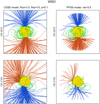 |
Fig. 2. CSSS (left column) and PFSS model (right column) magnetic field lines for Carrington rotations 2072 (first row) and 2150 (second row) based on WSO data, with Rcs = rss = 3.5, Rss = 10, and a = 0.1. Red lines denote open positive field, and blue lines denote open negative field. Green lines denote closed field. |
For the minimum time CR 2072 both models and both datasets produce large open polar regions and closed field lines at low latitudes. Especially for the maximum time CR 2150, the PFSS model produces larger areas of closed photospheric field lines. Moreover, during CR 2150, the PFSS field lines are bent more towards the poles, whereas in the CSSS model more field lines are bent towards the equator. This is because the CSSS model distributes the field lines latitudinally more evenly, which is due to its coronal current system (see also Fig. 3 in Zhao & Hoeksema 1994, where the PFSS field lines are shown to be more bent towards the poles than the HCCS model field lines). The field line configurations calculated using WSO data and SOLIS/VSM data are very similar in each case.
5. Latitude gradient
Figure 4 shows synoptic maps of the coronal field at the source surface for the CSSS model (Rcs = 3.5, Rss = 10, a = 0.1) and the PFSS model (rss = 3.5) for the two Carrington rotations depicted in Figs. 2 and 3, using WSO and SOLIS/VSM data. Figure 4 shows the notable difference in the latitude variation of the coronal field between these two models: the CSSS model gives a sharp boundary between the positive and negative field regions, whereas in the PFSS model the field is gradually reduced to zero over a wide latitude range before the sign changes. There is practically no difference in the location of the NL and HCS during CR 2072 (solar minimum) in the CSSS and PFSS models. Moreover, the location of the NL is very similar for the two datasets (WSO and SOLIS/VSM) during CR 2072. However, during solar maximum (CR 2150), the location of the NL and even the distributions of the field intensity are quite different in the CSSS and PFSS models. These variables also differ slightly in both models for the WSO and SOLIS/VSM data.
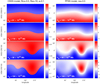 |
Fig. 4. Synoptic maps of the coronal source surface field (in μT) for the CSSS model (left column) and the PFSS model (right column), using WSO (first and third rows) and SOLIS/VSM (second and fourth rows) data for Carrington rotations 2072 (July 2008) and 2150 (May 2014). The total unsigned open flux ΦB is included in white font in each panel. Both nmax and nmax, c are 9. |
The total unsigned (open) flux ΦB noted in each panel in Fig. 4 is systematically some 30% higher in the PFSS model than in the CSSS model for these parameters. In both models the total unsigned flux with SOLIS/VSM data is approximately two to three times higher than the flux given by WSO data. This is due to the considerably higher spatial resolution of the SOLIS/VSM data. A roughly similar ratio was found for the dipole terms when we scaled harmonic coefficients between SOLIS/CSM and WSO data (Virtanen & Mursula 2017).
Furthermore, the maximum value of the field on the source surface in the CSSS model in Fig. 4 (about 0.25 μT) is more than one order of magnitude lower than for the PFSS model (about 7 μT). This is mostly because the source surface of the CSSS model in Fig. 4 is much farther out than the source surface of the PFSS model, but partly also because the field is distributed more evenly in the CSSS model than in the PFSS model.
Figure 5 shows the (rotational) longitudinal averages of the radial magnetic field on the source surface as a function of time (so-called supersynoptic maps) for the CSSS and PFSS models using WSO and the combined Kitt Peak (KP) and SOLIS/VSM data and the same model parameters as in Fig. 4. All panels include the full solar cycles 21, 22, and 23, and most of cycle 24. During the maximum of each cycle (1980, 1990, 2000, and 2014) the polarity of the field changes its sign both in the northern and southern hemispheres. In the CSSS model the field magnitude is fairly constant with latitude until it changes its sign over a narrow latitude range at the NL, near the equator. This is especially clear during the early ascending phase of the solar cycle. In the PFSS model the field is strongest at the poles, and decreases systematically towards lower latitudes, reaching zero at the NL. The average field magnitude is clearly lower after 2000, in the decreasing phase of cycle 23 than before this, during cycles 21 and 22. This is particularly clearly visible for WSO data in both models. In agreement with Fig. 4, the magnitude of the field in Fig. 5 is higher for combined KP and SOLIS/VSM data than for WSO data in the same model.
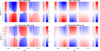 |
Fig. 5. Longitudinal averages of the coronal source surface field (in μT) for the CSSS model (Rss = 10, Rcs = 3.5, a = 0.1 Rs) (left panels) and the PFSS model (rss = 3.5) (right panels) as a function of time using WSO data (upper row) and Kitt Peak + SOLIS/VSM data (lower row). |
In order to study the latitude variation of the open flux for different parameters of the CSSS model, we calculated the radial field as a function of latitude at a constant longitude ϕ = 180°, using the CSSS model with Rcs = 3.5 and 5.5, Rss = 4.5, 7.5, 10, 12.5, 15, and 20, and a = 0.1, and compared them with the PFSS model result for rss = 3.5. Figure 6 shows these results for Carrington rotation 2072 (July 2008). In Fig. 6 the latitude where the radial field reaches zero is slightly shifted northwards of the equator because the NL at 180° longitude is shifted northwards, as shown in Fig. 4. If the difference between the cusp surface and source surface distances is small, the CSSS model gives a quite similar constantly varying latitude variation (with no large step between the two sectors) as the PFSS model (Fig. 6, panels 1 and 2, red curve). Increasing the difference between Rcs and Rss decreases the latitude gradient outside the HCS but sharpens the step at the HCS. For example, when Rcs = 3.5, a roughly constant field value outside the HCS (corresponding to Ulysses observations) is found for Rss ≥ 10. For Rcs = 5.5, the source surface distance must be even farther out, at least at 15, for the same condition to be fulfilled. Overall, it seems that it is necessary that Rss ≳ 3 × Rcs in order to achieve a roughly realistic latitudinal field variation of the open flux in the CSSS model.
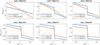 |
Fig. 6. Source surface radial field as a function of latitude at longitude ϕ = 180° for the CSSS model using WSO data for CR 2072. Parameter a = 0.1 in each panel, but Rcs and Rss values are varied. First panel: latitude trend of the PFSS model with rss = 3.5 for reference. The panels have different y-axis scales. |
6. Total flux
Figure 7 depicts the total open unsigned flux  for one Carrington rotation starting in each June from 1976 to 2017, varying Rcs from 1.5 to 6.5 and a from 0.01 to 3. Increasing the value of a increases the total flux, while increasing the value of Rcs decreases it (as discussed above). Figure 7 shows that when Rcs has a low value, increasing a increases the flux more steeply than for high Rcs values.
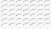 |
Fig. 7. Total open unsigned flux (in 1012 Wb) for WSO data as a function of a and Rcs for one Carrington rotation starting in each June from 1976 to 2017. The dotted vertical line marks Rcs = 3.5 and the dotted horizontal line marks a = 1. Rss has no effect on the open flux. |
Figure 8 shows a time series of the total open unsigned flux for the same rotations (one per year) as depicted in Fig. 7 using Rcs = 3.5, and a = 1 and 0.1. The flux value for a = 1 is approximately 30–50% higher than for a = 0.1, but the temporal variation of the total unsigned flux is very similar regardless of the value of a. Figure 8 depicts a clear variation over the solar cycle, with low values at solar maxima and high values in the declining phase of the solar cycle. The total unsigned flux has a notable long-term trend, with flux maxima decreasing from about 3.2 × 10¹⁴ Wb for a = 1 (about 2.2 × 10¹⁴ Wb for a = 0.1) in 1980s to about 1.6 × 10¹⁴ Wb for a = 1 (about 1.0 × 10¹⁴ Wb for a = 0.1) in 2010s. Correspondingly, the flux minima reduced from about 1.2 × 10¹⁴ Wb for a = 1 (about 0.7 × 10¹⁴ Wb for a = 0.1) in 1980 to about 0.8 × 10¹⁴ Wb for a = 1 (about 0.4 × 10¹⁴ Wb for a = 0.1) in 2015. Accordingly, the flux maxima decreased by roughly 50 % quite systematically during the past four cycles, but the reduction of flux minima was smaller and less systematic; the lowest values are found in 1999, not in the 2010s. Similar trends in flux maxima and minima were found by Wang et al. (2006).
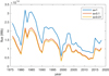 |
Fig. 8. Total open unsigned flux as a function of time for WSO data using Rcs = 3.5 and a = 1 (blue) and a = 0.01 (red), calculated for the same rotations as in Fig. 7. |
7. Neutral line
Figure 9 shows the source surface NL location for CR 2150 (May 2014) calculated for the CSSS model using WSO data and a range of CSSS parameters (a = 0.01, 0.1, 1; Rcs = 1.5, 3.5, 5.5; Rss = 5.5, 10.5, 15.5, 20.5). We compared the CSSS model results with the PFSS model and kept the PFSS source surface distance rss the same as Rcs of the CSSS model, as above.
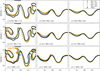 |
Fig. 9. Structure of the source surface NL during CR 2150 (May 2014) based on WSO data for a range of CSSS and PFSS model parameters. (Blue: Rss = 5.5, red: Rss = 10.5, yellow: Rss = 15.5, green: Rss = 20.5, and black: PFSS). The PFSS rss value is equal to the CSSS Rcs value in each panel. |
The first column shows the NL location with Rcs = rss = 1.5 and a values 0.01, 0.1, and 1. With this low cusp surface value, the NL shows a very complex multi-sheet structure for all values of a. When the cusp surface distance is increased to 3.5 (second column), the NL becomes flatter. Multiple NL structures disappear, but roughly the same large-scale pattern is sustained. For Rcs = 5.5Rs (third column) the NL becomes even slightly flatter. There is hardly any difference in the NL location between a = 0.01 (first row) and a = 0.1 (second row). For a = 1 the warps in the NL only become slightly larger for Rcs ≥ 3.5, but for Rcs = 1.5 the NL topology becomes even more complicated, and additional small-scale diversions appear.
Figure 9 shows that the different source surface values (shown in different colours in each panel) for most cases lead to very similar and often overlapping NL locations. This indicates that the source surface distance is almost negligible in determining the topology of the CSSS field.
The PFFS NL location (black curve in Fig. 9) follows the CSSS NL location quite well, although there are some differences, in particular for Rcs = rss = 1.5. However, even then the PFSS model produces a closely similar multi-sheet NL pattern, although the NL location is slightly shifted at some longitudes.
We conclude that the cusp surface distance has a dominant effect on the NL pattern and on the overall topology of the field in the CSSS model. The two other CSSS model parameters (a and Rss) have very little effect. The PFSS model produces a closely similar NL structure to that of the CSSS model when the same value is used for the PFSS rss and CSSS Rcs.
8. Polarity match
We have calculated the polarity match of magnetic fields by comparing the polarity of the field in the corona and at 1 AU (radial field in corona; plane division at 1 AU; see Koskela et al. 2017). We determined the source surface coordinates of the footpoint of a field line measured at 1 AU, and calculated the CSSS field solution at that location. We also used the Earth’s heliographic latitude at time t of the 1 AU measurement for the coronal source latitude. The source longitude was calculated by assuming that the solar wind moves radially outwards with a constant speed after it is emitted from the source surface. Thus, we calculated the time of transit Δt from the source surface to the Earth’s orbit using the solar wind speed observed at 1 AU. The source longitude is then the longitude of the central meridian of the Sun at time t − Δt. We determined the Carrington rotation that includes the time t − Δt, and used the synoptic map of that rotation to calculate the harmonic coefficients for the CSSS model. We then calculated the CSSS field at the correct source latitude and longitude, and compared the polarity (sign) of the coronal source field to the polarity (i.e. sector) of the magnetic field measured at 1 AU. We used hourly data, so that one rotation includes 648 comparisons. The polarity match is the percentage of hours that have the same polarity of the field at the two sites.
Figure 10 shows the polarity match for the minimum time rotation (CR 2076, October 2008) and the maximum time rotation (CR 2150, May 2014) with the following set of parameters: Rcs = 1.5−5.5, Rss = 2.5−19.5, Rss ≥ Rcs + 1, and a = 0.01, 0.1, 1. During CR 2076 the highest polarity match of 86–88% is obtained with Rcs ≈ 2.5, Rss ≳ 18 for a = 0.01 and 0.1, and Rcs = 2.5−3.5, Rss ≳ 18 for a = 1. During CR 2150 the highest polarity match of about 90% is obtained with a rather small range of parameters, Rcs = 2.5, Rss = 15−20 for a = 0.01, and Rcs = 3.5, Rss = 11−15 for 1 = 0.1. For a = 1, the highest polarity match remains below 90% for the studied parameter range.
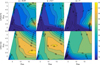 |
Fig. 10. Polarity match percentage (in colour coding and contour lines) for a range of parameters for CR 2076 (October 2008; upper row) and CR 2150 (May 2015; lower row). In each panel the vertical axis gives the Rcs value and the horizontal axis the Rss value. Each column has a different a value. |
We have searched for the optimal Rcs by calculating the polarity match for different Rcs values from 1.5 to 8.5, with a step of 0.25, and using Rss = 4 ⋅ Rcs and a = 0.01, 0.1, 1. The rotational polarity matches were calculated for all these 28 cusp surface distances and the three a values. We chose the Rcs value that provided the highest polarity match percentage for each rotation.
The two upper panels of Fig. 11 depict the rotational and the 13-rotation running means of the optimal Rcs values for a = 0.01, 0.1 and 1, as well as the 13-rotation running means of the PFSS optimal rss values as a reference. (The range of rss values was the same as for the Rcs, i.e. rss = 1.5−8.5, with a step of 0.25.). The number of rotations for which the optimal polarity match is obtained with Rcs = 8.5, i.e., at the boundary of the range of parameters, is 36 for a = 1 and 23 for a = 0.01 and 0.1, i.e. less than 7 % of all rotations. The first panel of Fig. 11 shows a high variation in the optimal cusp surface distance even between consecutive rotations. The second panel shows that the long-term variation of the three optimal Rcs curves is quite similar to that of the PFSS rss, but the Rcs values attain consistently lower values than rss. For a = 0.01 and a = 0.1 the optimal Rcs values almost overlap and differ significantly only in 1997, 2000–2002, and 2004. For a = 1 the optimal Rcs tends to be systematically higher than for the two lower a values. The optimal Rcs and rss tend to be relatively larger around solar minima (1977, 1985–1987, 1996–1997, and 2008–2009) and smaller around solar maxima or in the late ascending phase (1980–1981, 1990–1991, 1998–1999, and 2012). However, there is no clear (anti)correlation with sunspot cycle because additional peaks (and lows) are found in the declining phase, like in 1982, 1992, and 2002–2003.
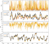 |
Fig. 11. Optimal Rcs for each Carrington rotation using WSO data. Rss is always 4 ⋅ Rcs and a is 0.01 (blue), 0.1 (red), or 1 (yellow). First panel: optimal Rcs. Second panel: thirteen-rotation running mean of the optimal Rcs. Third panel: polarity match with the optimal Rcs. Fourth panel: thirteen-rotation running mean of the polarity match. PFSS model results are included in the second and fourth panels (black). |
The polarity match (the two lower panels of Fig. 11) shows that the CSSS model only rarely produces a better polarity match with the optimal Rcs than the PFSS model with the best-ift rss. This is most clearly true in 1977, 1981, 2008, and 2010–2012. At all other times the CSSS model polarity match is equal to or even slightly weaker than the PFSS model polarity match. The PFSS model yields a better match most clearly in 1985, 1993, 1995, 2003, and 2006–2007. The three a values produce closely similar polarity match percentages, even when the optimal source surface distances are quite different. For example, the three CSSS models with different a values and the PFSS model yield a very similar polarity match (92–93%) in 2000, even though the optimal Rcs and rss values vary from 2.3 (for a = 0.1) to 3.9 (for a = 1) and 4.1 (for PFSS model).
9. Discussion and conclusions
We have studied the latitudinal variation and the strength of the unsigned open magnetic field, the coronal NL location, and the polarity match of the CSSS model for different parameter values, and compared them with those of the PFSS model. The range of all three CSSS model parameters, a, Rcs, and Rss, was allowed to be sufficiently large (a ≤ 1, Rcs < 9 and Rss < 20) so that all physically reasonable cases were covered.
The total flux is determined by two parameters of the CSSS model. It increases with increasing value of a and decreasing Rcs (Fig. 7). Especially for low Rcs values, the total flux increases rapidly with a. While very low (Rcs < 1.5) and very high Rcs > 6 values of Rcs are excluded, the total flux cannot yield an efficient limit for CSSS parameters because of problems related to instrument saturation (Svalgaard et al. 1978; Virtanen & Mursula 2017) and the partial viewing of poles (Sun et al. 2011), which directly affect the coronal flux. The total flux is determined by two parameters of the CSSS model. It increases with increasing value of a and decreasing Rcs (Fig. 7). Especially for low Rcs values, the total flux increases rapidly with a. While very low (Rcs < 1.5) and very high Rcs > 6 values of Rcs are excluded, the total flux cannot yield an efficient limit for CSSS parameters because of problems related to instrument saturation (Svalgaard et al. 1978; Virtanen & Mursula 2017) and the partial viewing of poles (Sun et al. 2011), which directly affect the coronal flux.
The greatest virtue of the CSSS model is that it can correct the systematic latitudinal change of the source surface field of the PFSS model, which is against Ulysses observations (Smith & Balogh 1995). Schüssler & Baumann (2006) noted that a roughly constant latitude profile is obtained when Rss = 10 and Rcs = 1.7. Using a comprehensive range of parameters, we found (Fig. 6) that the condition of a rather flat latitude variation of the source surface field constrains the ratio (not difference) between Rss and Rcs to being higher than about three. Thus, for typical values of Rcs = 2−4 the Rss has to be larger than about 6–12.
The NL structure depends very little on Rss and attains a closely similar pattern with the PFSS model when PFSS rss is taken to be the same as Rcs (see Fig. 9). We also found that the value of a has little effect upon the NL structure until it becomes quite high, close to a = 1, when it has the tendency of slightly increasing the warps of the NL. The cusp surface distance has the strongest effect upon the NL structure. For low values of Rcs ≤ 1.5, the NL tends to retain the typical multi-sheet structure of the maximum time photosphere. Because the NL of the HMF (the HCS) has a more simple structure even during solar maxima (Jones & Balogh 2003), this yields an effective lower limit to Rcs of about Rcs > 1.5. For high values of Rcs, the NL becomes more flat, but the change is rather slow, so that no strict upper limit can be found on Rcs from the NL structure.
Comparing the polarities of the magnetic field at 1 AU (HMF) and at the coronal source surface, we found that the CSSS model produces very similar optimal polarity match percentages as the PFSS model. While the CSSS model yields a better polarity match than the PFSS model for a few years, typically around solar minima or maxima, the PFSS model produces a better match than the CSSS model for roughly the same number of years, all found in the declining phase of the solar cycles. The long-term average polarity match with the CSSS model optimal Rcs is 85.6% for a = 0.01 and 0.1, 85.4% for a = 1, and with the PFSS model optimal rss 85.9%. For comparison, Li & Feng (2018) modelled the corona and heliosphere using a coupled coronal and heliospheric 3D MHD model, and obtained a polarity match of 85.8% in 2008. The polarity match we obtained for 2008 with the CSSS model optimal parameters was 88.2% for a = 0.01, 88.1% for a = 0.1, 88.4% for a = 1, and 87.4% for the PFSS model with the optimal rss.
The time evolution of the optimal Rcs is very similar to that of the optimal rss. Both the optimal Rcs and optimal rss tend to be be higher around solar minima and lower around solar maxima. However, the optimal Rcs is typically lower than the optimalrss, especially with the lowest a values used here (a = 0.01 and 0.1). The average values for optimal Rcs over the whole time period from 1976 to 2016 were 2.9 for a = 0.01, 3.0 for a = 0.1, and 3.6 for a = 1. The average optimal rss of the PFSS model was 3.9.
To conclude, the CSSS model, as a few other models including a current sheet such as the PFCS and HCCS models, corrects the erroneous latitude variation of the PFSS model if the source surface distance is at least three times the cusp surface distance. Thus, these models are preferred over the PFSS model when the coronal or HMF field outside the equator (or ecliptic) is studied. However, when the topology of the magnetic field (e.g., the structure of the NL or the distribution of polarities) is studied, the PFSS model is sufficient because the CSSS model is not able to systematically improve the polarity match between the coronal field and the HMF. We find that the optimal Rcs values lie within 2–4 solar radii for a ≤ 0.1 and 2.5–4.5 solar radii for a ≈ 1. Both the optimal Rcs value and the optimal polarity match depict a closely similar long-term evolution for all values of a, as well as for the PFSS model. Accordingly, none of the studied constraints can effectively narrow down the possible range of the a parameter of the CSSS model within a ≤ 1. Thus, from the practical point of view, adding purely horizontal currents in the model seems to be an unnecessary complication for the constraints studied here. This conclusion is not valid for a more complicated or realistic set of coronal currents.
Acknowledgments
We acknowledge the financial support by the Academy of Finland to the ReSoLVE Centre of Excellence (project no. 307411). The Wilcox Solar Observatory data used in this study were obtained via the website http://wso.stanford.edu courtesy of J. T. Hoeksema. SOLIS/VSM data were acquired by SOLIS instruments operated by NISP/NSO/AURA/NSF. NSO/Kitt Peak magnetic data used here are produced cooperatively by NSF/NOAO, NASA/GSFC and NOAA/SEL. The data used in this study were obtained from the following websites: WSO: http://wso.stanford.edu KP: ftp://solis.nso.edu/kpvt/synoptic/mag/ SOLIS/VSM: http://solis.nso.edu
References
- Altschuler, M. D., & Newkirk, G. 1969, Sol. Phys., 9, 131 [Google Scholar]
- Bogdan, T. J., & Low, B. C. 1986, ApJ, 306, 271 [NASA ADS] [CrossRef] [Google Scholar]
- Contopoulos, I., Kalapotharakos, C., & Georgoulis, M. K. 2011, Sol. Phys., 269, 351 [NASA ADS] [CrossRef] [Google Scholar]
- Jones, G. H., & Balogh, A. 2003, Ann. Geophys., 21, 1377 [NASA ADS] [CrossRef] [Google Scholar]
- Koskela, J. S., Virtanen, I. I., & Mursula, K. 2017, ApJ, 835, 63 [NASA ADS] [CrossRef] [Google Scholar]
- Li, H., & Feng, X. 2018, J. Geophys. Res. (Space Phys.), 123, 4488 [Google Scholar]
- Lockwood, M., Rouillard, A. P., Finch, I., & Stamper, R. 2006, J. Geophys. Res. (Space Phys.), 111, A09109 [NASA ADS] [Google Scholar]
- Low, B. C. 1985, ApJ, 293, 31 [NASA ADS] [CrossRef] [Google Scholar]
- Low, B. C. 1991, ApJ, 370, 427 [NASA ADS] [CrossRef] [Google Scholar]
- Mackay, D. H., & Yeates, A. R. 2012, Liv. Rev. Sol. Phys., 9, 6 [Google Scholar]
- Neukirch, T. 1995, A&A, 301, 628 [NASA ADS] [Google Scholar]
- Parker, E. N. 1958, ApJ, 128, 664 [Google Scholar]
- Pneuman, G. W., & Kopp, R. A. 1970, Sol. Phys., 13, 176 [NASA ADS] [CrossRef] [Google Scholar]
- Pneuman, G. W., & Kopp, R. A. 1971, Sol. Phys., 18, 258 [NASA ADS] [CrossRef] [Google Scholar]
- Poduval, B. 2016, ApJ, 827, L6 [NASA ADS] [CrossRef] [Google Scholar]
- Poduval, B., & Zhao, X. P. 2014, ApJ, 782, L22 [NASA ADS] [CrossRef] [Google Scholar]
- Riley, P., Linker, J. A., Mikic, Z., et al. 2006, ApJ, 653, 1510 [Google Scholar]
- Riley, P., Linker, J. A., & Arge, C. N. 2015, Space Weather, 13, 154 [NASA ADS] [CrossRef] [Google Scholar]
- Schatten, K. H. 1972, NASA Spec. Publ., 308, 44 [NASA ADS] [Google Scholar]
- Schatten, K. H., Wilcox, J. M., & Ness, N. F. 1969, Sol. Phys., 6, 442 [Google Scholar]
- Schüssler, M., & Baumann, I. 2006, A&A, 459, 945 [NASA ADS] [CrossRef] [EDP Sciences] [Google Scholar]
- Smith, E. J., & Balogh, A. 1995, Geophys. Res. Lett., 22, 3317 [NASA ADS] [CrossRef] [Google Scholar]
- Sun, X., Liu, Y., Hoeksema, J. T., Hayashi, K., & Zhao, X. 2011, Sol. Phys., 270, 9 [NASA ADS] [CrossRef] [Google Scholar]
- Svalgaard, L., Duvall, Jr., T. L., & Scherrer, P. H. 1978, Sol. Phys., 58, 225 [Google Scholar]
- Virtanen, I., & Mursula, K. 2016, A&A, 591, A78 [NASA ADS] [CrossRef] [EDP Sciences] [Google Scholar]
- Virtanen, I., & Mursula, K. 2017, A&A, 604, A7 [NASA ADS] [CrossRef] [EDP Sciences] [Google Scholar]
- Wang, Y.-M., & Sheeley, Jr., N. R. 1990, ApJ, 355, 726 [Google Scholar]
- Wang, Y.-M., & Sheeley, Jr., N. R. 1997, Geophys. Res. Lett., 24, 3141 [NASA ADS] [CrossRef] [Google Scholar]
- Wang, Y.-M., Sheeley, Jr., N. R., & Rouillard, A. P. 2006, ApJ, 644, 638 [NASA ADS] [CrossRef] [Google Scholar]
- Wiegelmann, T. 2007, Sol. Phys., 240, 227 [NASA ADS] [CrossRef] [Google Scholar]
- Yeates, A. R., Amari, T., Contopoulos, I., et al. 2018, Space Sci. Rev., 214, 99 [Google Scholar]
- Zhao, X. P., & Hoeksema, J. T. 1992, in Coronal Streamers, Coronal Loops, and Coronal and Solar Wind Composition, ed. C. Mattok, ESA Spec. Publ., 348, 412 [Google Scholar]
- Zhao, X., & Hoeksema, J. T. 1994, Sol. Phys., 151, 91 [Google Scholar]
- Zhao, X., & Hoeksema, J. T. 1995, J. Geophys. Res., 100, 19 [NASA ADS] [CrossRef] [Google Scholar]
All Figures
|
Fig. 1. Sketch of the CSSS model. The inner black circle is the photosphere, the middle circle is the cusp surface, and the outer circle is the source surface. At the cusp surface the field lines become open and at the source surface they become radial. The field lines that remain beneath the cusp surface are closed field lines. Red lines denote away-field, blue lines towards-field, and green lines are closed. |
| In the text | |
|
Fig. 2. CSSS (left column) and PFSS model (right column) magnetic field lines for Carrington rotations 2072 (first row) and 2150 (second row) based on WSO data, with Rcs = rss = 3.5, Rss = 10, and a = 0.1. Red lines denote open positive field, and blue lines denote open negative field. Green lines denote closed field. |
| In the text | |
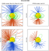 |
Fig. 3. Same as Fig. 2 using SOLIS/VSM data. |
| In the text | |
|
Fig. 4. Synoptic maps of the coronal source surface field (in μT) for the CSSS model (left column) and the PFSS model (right column), using WSO (first and third rows) and SOLIS/VSM (second and fourth rows) data for Carrington rotations 2072 (July 2008) and 2150 (May 2014). The total unsigned open flux ΦB is included in white font in each panel. Both nmax and nmax, c are 9. |
| In the text | |
|
Fig. 5. Longitudinal averages of the coronal source surface field (in μT) for the CSSS model (Rss = 10, Rcs = 3.5, a = 0.1 Rs) (left panels) and the PFSS model (rss = 3.5) (right panels) as a function of time using WSO data (upper row) and Kitt Peak + SOLIS/VSM data (lower row). |
| In the text | |
|
Fig. 6. Source surface radial field as a function of latitude at longitude ϕ = 180° for the CSSS model using WSO data for CR 2072. Parameter a = 0.1 in each panel, but Rcs and Rss values are varied. First panel: latitude trend of the PFSS model with rss = 3.5 for reference. The panels have different y-axis scales. |
| In the text | |
|
Fig. 7. Total open unsigned flux (in 1012 Wb) for WSO data as a function of a and Rcs for one Carrington rotation starting in each June from 1976 to 2017. The dotted vertical line marks Rcs = 3.5 and the dotted horizontal line marks a = 1. Rss has no effect on the open flux. |
| In the text | |
|
Fig. 8. Total open unsigned flux as a function of time for WSO data using Rcs = 3.5 and a = 1 (blue) and a = 0.01 (red), calculated for the same rotations as in Fig. 7. |
| In the text | |
|
Fig. 9. Structure of the source surface NL during CR 2150 (May 2014) based on WSO data for a range of CSSS and PFSS model parameters. (Blue: Rss = 5.5, red: Rss = 10.5, yellow: Rss = 15.5, green: Rss = 20.5, and black: PFSS). The PFSS rss value is equal to the CSSS Rcs value in each panel. |
| In the text | |
|
Fig. 10. Polarity match percentage (in colour coding and contour lines) for a range of parameters for CR 2076 (October 2008; upper row) and CR 2150 (May 2015; lower row). In each panel the vertical axis gives the Rcs value and the horizontal axis the Rss value. Each column has a different a value. |
| In the text | |
|
Fig. 11. Optimal Rcs for each Carrington rotation using WSO data. Rss is always 4 ⋅ Rcs and a is 0.01 (blue), 0.1 (red), or 1 (yellow). First panel: optimal Rcs. Second panel: thirteen-rotation running mean of the optimal Rcs. Third panel: polarity match with the optimal Rcs. Fourth panel: thirteen-rotation running mean of the polarity match. PFSS model results are included in the second and fourth panels (black). |
| In the text | |
Current usage metrics show cumulative count of Article Views (full-text article views including HTML views, PDF and ePub downloads, according to the available data) and Abstracts Views on Vision4Press platform.
Data correspond to usage on the plateform after 2015. The current usage metrics is available 48-96 hours after online publication and is updated daily on week days.
Initial download of the metrics may take a while.