| Issue |
A&A
Volume 631, November 2019
|
|
|---|---|---|
| Article Number | A157 | |
| Number of page(s) | 25 | |
| Section | Extragalactic astronomy | |
| DOI | https://doi.org/10.1051/0004-6361/201832882 | |
| Published online | 13 November 2019 | |
Stellar populations of galaxies in the ALHAMBRA survey up to z ∼ 1
III. The stellar content of the quiescent galaxy population during the last 8 Gyr⋆
1
Centro de Estudios de Física del Cosmos de Aragón (CEFCA), Plaza San Juan 1, Floor 2, 44001 Teruel, Spain
e-mail: This email address is being protected from spambots. You need JavaScript enabled to view it.
2
Academia Sinica Institute of Astronomy & Astrophysics (ASIAA), 11F of Astronomy-Mathematics Building, AS/NTU, No. 1, Section 4, Roosevelt Road, Taipei 10617, Taiwan
3
Centro de Estudios de Física del Cosmos de Aragón (CEFCA) – Unidad Asociada al CSIC, Plaza San Juan 1, Floor 2, 44001 Teruel, Spain
4
Mullard Space Science Laboratory, University College London, Holmbury St Mary, Dorking, Surrey RH5 6NT, UK
5
Instituto de Física de Cantabria (CSIC-UC), 39005 Santander, Spain
6
Unidad Asociada Observatorio Astronómico (IFCA-UV), 46980 Paterna, Spain
7
IAA-CSIC, Glorieta de la Astronomía s/n, 18008 Granada, Spain
8
Instituto de Astrofísica de Canarias, Vía Láctea s/n, 38200 La Laguna, Tenerife, Spain
9
Observatório Nacional-MCT, Rua José Cristino, 77, 20921-400 Rio de Janeiro, RJ, Brazil
10
Department of Theoretical Physics, University of the Basque Country UPV/EHU, 48080 Bilbao, Spain
11
Ikerbasque, Basque Foundation for Science, Bilbao, Spain
12
Departamento de Física Atómica, Molecular y Nuclear, Facultad de Física, Universidad de Sevilla, 41012 Sevilla, Spain
13
Institut de Ciències de l’Espai (IEEC-CSIC), Facultat de Ciències, Campus UAB, 08193 Bellaterra, Spain
14
Departamento de Astrofísica, Facultad de Física, Universidad de La Laguna, 38206 La Laguna, Spain
15
Instituto de Astrofísica, Universidad Católica de Chile, Av. Vicuna Mackenna 4860, 782-0436 Macul, Santiago, Chile
16
Centro de Astro-Ingeniería, Universidad Católica de Chile, Av. Vicuna Mackenna 4860, 782-0436 Macul, Santiago, Chile
17
Observatori Astronòmic, Universitat de València, C/ Catedràtic José Beltrán 2, 46980 Paterna, Spain
18
Departament d’Astronomia i Astrofísica, Universitat de València, 46100 Burjassot, Spain
19
Instituto de Astronomía, Geofísica e Ciéncias Atmosféricas, Universidade de São Paulo, São Paulo, Brazil
Received:
22
February
2018
Accepted:
7
June
2019
Abstract
Aims. We aim at constraining the stellar population properties of quiescent galaxies. These properties reveal how these galaxies evolved and assembled since z ∼ 1 up to the present time.
Methods. Combining the ALHAMBRA multi-filter photo-spectra with the fitting code for spectral energy distribution MUFFIT (MUlti-Filter FITting), we built a complete catalogue of quiescent galaxies via the dust-corrected stellar mass vs. colour diagram. This catalogue includes stellar population properties, such as age, metallicity, extinction, stellar mass, and photometric redshift, retrieved from the analysis of composited populations based on two independent sets of simple stellar population (SSP) models. We developed and applied a novel methodology to provide, for the first time, the analytic probability distribution functions (PDFs) of mass-weighted age, metallicity, and extinction of quiescent galaxies as a function of redshift and stellar mass. We adopted different star formation histories to discard potential systematics in the analysis.
Results. The number density of quiescent galaxies is found to increase since z ∼ 1, with a more substantial variation at lower stellar mass. Quiescent galaxies feature extinction AV < 0.6, with median values in the range AV = 0.15–0.3. At increasing stellar mass, quiescent galaxies are older and more metal rich since z ∼ 1. A detailed analysis of the PDFs reveals that the evolution of quiescent galaxies is not compatible with passive evolution and a slight decrease of 0.1–0.2 dex is hinted at median metallicity. The intrinsic dispersion of the age and metallicity PDFs show a dependence on stellar mass and/or redshift. These results are consistent with both sets of SSP models and assumptions of alternative star formation histories explored. Consequently, the quiescent population must undergo an evolutive pathway including mergers and/or remnants of star formation to reconcile the observed trends, where the “progenitor” bias should also be taken into account.
Key words: galaxies: stellar content / galaxies: photometry / galaxies: evolution / galaxies: formation
Based on observations collected at the Centro Astronómico Hispano Alemán (CAHA) at Calar Alto, operated jointly by the Max-Planck Institut für Astronomie and the Instituto de Astrofísica de Andalucía (CSIC).
© ESO 2019
1. Introduction
Over the past two decades, many authors have found that galaxies lie on two well-differentiated groups or colour distributions (e.g. Bell et al. 2004; Baldry et al. 2004; Williams et al. 2009; Ilbert et al. 2010; Peng et al. 2010; Arnouts et al. 2013; Moresco et al. 2013; Fritz et al. 2014). This bimodality can be interpreted in terms of differences of either the stellar content of the galaxies, or variations in their evolutive pathways. In this sense, red galaxies typically exhibit evolved stellar populations with low levels of star formation, and are termed quiescent, passive, or even “dead” galaxies. The formation and evolution of the so-called quiescent galaxies remains a challenge to date, as these galaxies started to form stars at very early epochs, shutting down their star formation at later times by mechanisms that are still open to debate (Faber et al. 2007; Peng et al. 2010; Ilbert et al. 2013; Peng et al. 2015; Barro et al. 2016). One of the most extended and promising approaches to determining the star formation history (SFH) of quiescent galaxies is the study of the evolution of their stellar population content with cosmic time.
Many authors focused on the SFH of galaxies in low redshift samples. This is typically termed the “archaeological” approach or fossil record method. This method has been extensively used to assess the stellar content of galaxies through either integrated properties or spatially-resolved observations (e.g. Cid Fernandes et al. 2005; Gallazzi et al. 2005; Thomas et al. 2005; Rogers et al. 2010; de La Rosa et al. 2011; Trevisan et al. 2012; Ferré-Mateu et al. 2013; Conroy et al. 2014; Trujillo et al. 2014; Belli et al. 2015; McDermid et al. 2015; González Delgado et al. 2015; Citro et al. 2016; Zheng et al. 2017; Goddard et al. 2017; González Delgado et al. 2017). The analysis is based on the (full) spectral energy distribution (SED) fitting or on targeted spectral indices that are sensitive to parameters such as age, metallicity, α enhancement, IMF, etc. These methods usually adopt stellar population models with different SFHs, including bursts of various durations. Alternatively to the fossil record method, the comparison between the stellar populations of similar samples at high and low redshifts (termed the “look-back” approach) provides complementary constraints to galaxy evolution (e.g. Schiavon et al. 2006; van Dokkum 2008; Sánchez-Blázquez et al. 2009a; Choi et al. 2014; Gallazzi et al. 2014; Jørgensen et al. 2014; Fagioli et al. 2016; Gargiulo et al. 2017; Kriek et al. 2016; Siudek et al. 2017). Whilst the look-back studies constitute a direct comparison between distributions of galaxies at different redshift, any interpretation of the results is limited by the “progenitor” bias (a term introduced by van Dokkum & Franx 2001). Consequently, samples of galaxies at high redshift are biased subsets of the nearby counterparts, because the former only includes the oldest members of the current distributions. In fact, recent studies point out that there has been an increasing number of quiescent galaxies since z ∼ 3, supporting the idea that samples of quiescent galaxies at high or intermediate redshift are largely biased when compared to their low redshift counterpart (e.g. Drory et al. 2009; Pozzetti et al. 2010; Ilbert et al. 2010; Brammer et al. 2011; Cassata et al. 2011; Davidzon et al. 2013; Ilbert et al. 2013; Moustakas et al. 2013; Moresco et al. 2013; Tomczak et al. 2014). Other recent results advocate a reduction in the number of massive star-forming galaxies (Bell et al. 2007; Davidzon et al. 2013; Ilbert et al. 2013; Moustakas et al. 2013), a hypothesis that also explains the observational size growth of massive quiescent galaxies (e.g. van Dokkum et al. 2008; Shankar & Bernardi 2009; Belli et al. 2015; Fagioli et al. 2016; Gargiulo et al. 2017; McDermid et al. 2015; Williams et al. 2017) and the scatter in the red sequence (RS; Harker et al. 2006; Ruhland et al. 2009).
Some of these quiescent galaxies are very old (see e.g. Jørgensen & Chiboucas 2013; Whitaker et al. 2013) and would have undergone a very efficient process of star formation, followed by fast quenching, because the sequence of quiescent galaxies is already in place at z ∼ 3 (van Dokkum et al. 2003; Kriek et al. 2006, 2008; van Dokkum & Brammer 2010a; Whitaker et al. 2011, 2013; Ilbert et al. 2013). Some authors have dedicated large efforts to studying their evolution over a long period of time, amongst others, through the study of their star formation rates (Papovich et al. 2006; Martin et al. 2007; Zheng et al. 2007; Pérez-González et al. 2008; Damen et al. 2009; Barro et al. 2014a), studying the evolution of their number density with cosmic time (Cimatti et al. 2006; Ferreras et al. 2009a,b; Ilbert et al. 2010, 2013; Pozzetti et al. 2010; Brammer et al. 2011; Moustakas et al. 2013), or attempting to reconstruct their SFH by fossil record methods (Heavens et al. 2004; Thomas et al. 2005; Jimenez et al. 2007; Barro et al. 2014b; McDermid et al. 2015; González Delgado et al. 2017). Overall, there is good agreement in that the evolution of these galaxies strongly depends on the stellar mass (largely studied at low and intermediate redshift, e.g. Ferreras & Silk 2000; Kauffmann et al. 2003; Gallazzi et al. 2005; Thomas et al. 2005; Sánchez-Blázquez et al. 2006; Jimenez et al. 2007; Kaviraj et al. 2007; Panter et al. 2008; Vergani et al. 2008; Ferreras et al. 2009a,c; van Dokkum & Conroy 2010b; de La Rosa et al. 2011; González Delgado et al. 2014a; Peng et al. 2015; Whitaker et al. 2017) and more slightly on the environment or morphology (e.g. Thomas et al. 2005; Ferreras et al. 2006; Rogers et al. 2010; La Barbera et al. 2014; González Delgado et al. 2015, 2017; McDermid et al. 2015). In this sense, the more massive galaxies were formed at earlier epochs owing to a more efficient and quicker process of star formation, meaning “downsizing” (Cowie et al. 1996). In addition, there is good agreement on the presence of a tight and positive correlation between the gas-phase metallicity and the stellar mass (e.g. Tremonti et al. 2004; Savaglio et al. 2005; Erb et al. 2006; Lee et al. 2006), that can be also extended to total stellar metallicity (Gallazzi et al. 2005, 2014; González Delgado et al. 2014b; Peng et al. 2015), a trend called the stellar mass–metallicity relation (MZR, with distinction between the gas-phase metallicity and the total stellar metallicity). This relation has been confirmed in studies at intermediate redshift (e.g. Sánchez-Blázquez et al. 2009a; Gallazzi et al. 2014; Jørgensen et al. 2017). Nevertheless, some authors point out that there are more relevant parameters than stellar mass as drivers of the stellar populations of galaxies (Díaz-García et al. 2019b), such as the stellar surface density (Kauffmann et al. 2003; Franx et al. 2008) or central velocity dispersion (Trager et al. 2000; Gallazzi et al. 2006; Graves & Faber 2010; Cappellari et al. 2013).
Although strong, in-situ star formation episodes are widely accepted to be a relevant channel contributing to galaxy formation, observations suggest that other mechanisms, such as mergers, can also contribute significantly (see e.g. Toomre 1977; Schweizer & Seitzer 1992; Barnes & Hernquist 1996; Trager et al. 2000; Benson et al. 2003; Croton et al. 2006; Khochfar & Silk 2006; Somerville et al. 2008; Hopkins et al. 2008; Ferreras et al. 2009a; Hopkins et al. 2009; van der Wel et al. 2009; Skelton et al. 2012; Díaz-García et al. 2013; López-Sanjuan et al. 2013; Ferreras et al. 2014). Once star formation is quenched or strongly reduced, these mechanisms may be important drivers of galaxy evolution. A detailed analysis of the stellar content of quiescent galaxies can unveil these mechanisms, as well as how galaxies evolve once they slow down or quench their star formation activity. Not only is the evolution of median values of stellar population properties clearly relevant, but also the intrinsic dispersions of these values, which can be tightly related to mechanisms modifying the stellar content of galaxies.
In this context, the state-of-the-art, multi-filter surveys, for example COMBO-171 (Wolf et al. 2003), MUSYC2 (Gawiser et al. 2006), COSMOS3 (Scoville et al. 2007), ALHAMBRA4 (Moles et al. 2008), CLASH5 (Postman et al. 2012), SHARDS6 (Pérez-González et al. 2013), J-PAS7 (Benítez et al. 2014), and J-PLUS8 (Cenarro et al. 2019) can provide an alternative way to explore the stellar content of galaxies through SED-fitting techniques (Mathis et al. 2006; Koleva et al. 2008; Walcher et al. 2011; Díaz-García et al. 2015; Ruiz-Lara et al. 2015) beyond the present day Universe. These photometric surveys, typically deeper than spectroscopy, can easily observe large samples of galaxies at intermediate redshift (z ∼ 1–2). This allows us to set milestones on the assembly of the stellar content of quiescent galaxies, offering a more continuous view of galaxy formation than the fossil record approach, as the former method proposes a sequence of “snapshots” across cosmic time. Moreover, multi-filter photometric surveys that combine narrow and medium bands, whose data are defined as photo-spectra, offer remarkable advantages: (i) there is no sampling bias other than the photometric depth of the detection band; (ii) independent photometric calibration can be obtained of each band; (iii) the photometric depth is usually much deeper than spectroscopic surveys with similar telescopes; (iv) photometry is not affected by aperture bias, as dynamical apertures are used to collect all the flux from the sources; (v) large scale multi-filter surveys provide a photo-spectrum at each pixel on the sky, enabling us to spatially (2D) explore resolved sources (Ferreras et al. 2005; San Roman et al. 2017); and (vi) large samples of galaxies across a wide redshift range allow unbiased statistical studies, where the various systematics can be mitigated owing to the large number of sources.
This work is part of a series of papers focused on the formation and evolution of quiescent galaxies since z ∼ 1, making use of multiple observables (e.g. co-moving number densities, stellar population properties, and sizes). In this paper, we study the stellar content of quiescent galaxies from the ALHAMBRA multi-filter survey to constrain their properties, and we also set limits on the range of values found. For the first time, we build the probability distribution functions (PDFs) of stellar age, metallicity, and dust extinction in quiescent galaxies since z ∼ 1, including their number densities in our analysis to provide a general picture of how these galaxies evolve once star formation is quenched. This is a unique opportunity to explore alternative mechanisms, for example as a result of their closest environment or by mergers, modifying the stellar content of galaxies that may remain unnoticed under an efficient in-situ star formation of the host galaxy.
This paper is structured as follows. In Sect. 2, we briefly explain the selection of the quiescent galaxy sample from the ALHAMBRA survey, and we also provide basic details of the ALHAMBRA data, SED-fitting techniques, and the main ingredients to determine the stellar population properties involved in this work. The co-moving number densities of quiescent galaxies from ALHAMBRA are presented in Sect. 3. The main results of this work, namely, the constraints found on the stellar content of quiescent galaxies since z ∼ 1 and their evolution with redshift are detailed in Sect. 4. We discuss and compare our results in Sects. 5 and 6, respectively. The conclusions are briefly summarised in Sect. 7.
Throughout this work a Lambda cold dark matter (ΛCDM) cosmology is adopted, with H0 = 71 km s−1, ΩM = 0.27, and ΩΛ = 0.73. Stellar masses are quoted in solar mass units [M⊙] and magnitudes in the AB-system (Oke & Gunn 1983). In this work, we assumed Chabrier (2003) and Kroupa Universal (Kroupa 2001) initial stellar mass functions (IMF, more details in Sect. 2.2).
2. Sample of quiescent galaxies
Our parent catalogue is the sample of quiescent galaxies of Díaz-García et al. (2019a; hereafter DG17). This catalogue is complete in stellar mass and in magnitude, down to I = 23 and contains ∼8500 quiescent galaxies from the multi-filter ALHAMBRA survey9 over a redshift range of 0.1 ≤ z ≤ 1.1. To select quiescent galaxies, DG17 performed a dust-corrected stellar mass–colour diagram (MCDE) on a general sample of ∼90 000 galaxies. This diagram has been shown to be a reliable diagnostic to substantially reduce the contamination of dusty star-forming galaxies (details in DG17). The DG17 catalogue includes stellar population properties, retrieved by use of different SSP models via SED-fitting. The properties include mass- and luminosity-weighted ages and metallicities, stellar masses, dust extinction, photo-z, rest-frame luminosities, colours corrected for extinction, and the parameter uncertainties. Below, we briefly detail the main features of the ALHAMBRA data set (Sect. 2.1) and the methodology used to retrieve the stellar population properties of quiescent galaxies (Sect. 2.2).
2.1. The ALHAMBRA photometric data
The ALHAMBRA survey provides flux in 23 photometric bands10 (Coe et al. 2006, corrected for point spread function), 20 in the optical wavelength range λλ 3500–9700 Å (top hat medium-band filters, ∼300 Å full width at half maximum, overlapping close to zero between contiguous bands; see Aparicio Villegas et al. 2010) and 3 in the near-infrared (NIR) spectral window λλ 1.0–2.3 μm (J, H, and Ks bands; further details in Cristóbal-Hornillos et al. 2009) for each source in 7 non-contiguous fields along the northern hemisphere. The current effective area of the survey is ∼2.8 deg2, acquired at the 3.5 m telescope of the Calar Alto Observatory11 (CAHA). The observations in the optical range were performed with the wide-field camera LAICA12 (4 CCDs of 4096 × 4096 pixels and pixel scale 0.225″ pixel−1) and with Omega-200013 (1CCD with 2048 × 2048 pixels and plate scale 0.45″ pixel−1) in the NIR regime. We adopted the ALHAMBRA Gold catalogue14 (Molino et al. 2014) as the reference photometric data set. This catalogue contains ∼95 000 galaxies imaged in 20 + 3 optical and NIR bands, respectively. The Gold catalogue provides accurate photometry (non-fixed aperture), needed to undertake stellar population studies (Díaz-García et al. 2015). It is supplemented with precise photo-z predictions (σz ∼ 0.012), down to I = 23.
2.2. Stellar population properties of quiescent galaxies
In order to retrieve the stellar population parameters of quiescent galaxies in the DG17 catalogue, we ran the code MUFFIT (MUlti-Filter FITting for stellar population diagnostics, Díaz-García et al. 2015). This code has proven a reliable tool to constrain the stellar content of galaxies from multi-filter photometric data (Díaz-García et al. 2015). MUFFIT builds composite models of stellar populations (mixtures of two SSPs) from SSP sets. In this work we separately use two independent sets of SSP models to construct two samples of composite models of stellar populations, allowing us to assess potential systematics caused by the differing model prescriptions between these sets. The first set comprises the Bruzual & Charlot (2003) SSP models (hereafter BC03); stellar age from 0.06 to 14 Gyr, metallicities [M/H] = − 1.65, −0.64, −0.33, 0.09, 0.55 (Padova 1994 tracks), and assuming a Chabrier (2003) initial-mass function. The second set comprises the Vazdekis et al. (2016) SSP models (EMILES15, λλ 1680 Å–5 μm), that is the UV and NIR extension of Vazdekis et al. (2012) SSP models (MIUSCAT, see also Vazdekis et al. 2003, 2010). In the EMILES models, the two sets of theoretical isochrones adopted by the authors were taken into account: the scaled-solar isochrones of Girardi et al. (2000; hereafter Padova00) and Pietrinferni et al. (2004, BaSTI in the following). For this set, we took 22 ages in the range of 0.05–14 Gyr and metallicities [M/H] = − 1.31, −0.71, −0.40, 0.00, 0.22 for Padova00 and [M/H] = − 1.26, −0.96, −0.66, −0.35, 0.06, 0.26, 0.40 for BaSTI, both with the Kroupa Universal IMF (Kroupa 2001). It should be noted that as shown by DG17, stellar masses of quiescent galaxies retrieved through MUFFIT and EMILES SSP models are systematically higher, ∼0.1 dex, than those derived from the BC03 models. For this reason, compatible stellar mass bins between EMILES and BC03 predictions differ by 0.1 dex throughout this work. In all sets of SSP models, dust attenuation was added as a foreground screen16 to the SSPs with values in the range AV = 0.0–3.1, following the Milky Way extinction law of Fitzpatrick (1999), and assuming a fixed value of RV = 3.1. In addition, we only used SSP models with cosmologically consistent ages to produce the sample of composite models of stellar populations, that is, they cannot be older than the age of the Universe at any redshift, adopting a ΛCDM cosmology. However, this constraint on age did not alter our results significantly.
Discrepancies between luminosity- and mass-weighted parameters from composite stellar population models can be particularly relevant (Ferreras & Yi 2004; Serra & Trager 2007; Rogers et al. 2010). Throughout this work, the mass-weighted ages and metallicities (AgeM and [M/H]M, respectively) are preferred to the luminosity-weighted ones. The mass-weighted parameters are more physically motivated and representative of the total stellar content of the galaxy. Moreover, mass-weighted properties are not linked to a definition of luminosity weight, which may differ amongst different studies. However, luminosity-weighted parameters are also estimated. Look-back times were established following the recipes by Hogg (1999). Hereafter, we define the formation epoch as the sum of the mass-weighted age and look-back time (AgeM + tLB).
3. Number density of quiescent galaxies
Co-moving number densities, ρN, can be a powerful tool to set constraints on the evolution of quiescent galaxies, as well as to provide hints about the characteristic timescales of the processes involved. To derive co-moving number densities, we made use of the 1/Vmax formalism (Schmidt 1968) in the sub-samples that are complete in stellar mass (see DG17 for details). The errors of ρN are estimated by the error propagation of the 1/Vmax method, given by Poisson errors (in accordance with similar previous assumptions, e.g. Marshall 1985; Ilbert et al. 2005). It is worth mentioning that additional uncertainties owing to cosmic variance are also included in the error budget (see also López-Sanjuan et al. 2015), for which we followed the recipe detailed in Moster et al. (2011). Our estimations point out that the relative cosmic variance of the ALHAMBRA sample stays at a 5–7% fraction.
The evolution of the number density of quiescent galaxies is summarised in Table 1 and illustrated in Fig. 1. We found that there is a generalised lack of galaxies at z ∼ 0.6, independent of the stellar mass and more noticeable in the BC03 SSP models (see panel a in Fig. 1). In order to ensure that this lack of galaxies is not systematically introduced by our technique, we checked that the number density of the whole population of galaxies in ALHAMBRA also present a lack of galaxies. To support this idea and as sanity check, we studied the distribution of photo-z provided by the parent Gold catalogue instead of the one provided by MUFFIT, and those provided making use of other independent photo-z codes, EAZY (Easy and Accurate z-phot from Yale, Brammer et al. 2008) and LePHARE (Photometric Analysis for redshift estimations code, Arnouts et al. 2002; Ilbert et al. 2006). For EAZY, we allowed the combination of its default templates; whereas for LePHARE we chose the COSMOS SED templates, that include dust extinction. Similarly to BPZ (Bayesian Photometric Redshift, Benítez 2000), both codes can apply constraints on the redshift distribution during the χ2 fitting procedure, which has been shown to improve the photo-z estimates (e.g. Benítez 2000; Ilbert et al. 2006; Brammer et al. 2008). We assumed the default priors of each code: for EAZY the prior is on the R band, and for LePHARE it is applied on the I band. After running EAZY and LePHARE, the retrieved photo-z distributions are analysed separately for the quiescent and star-forming sub-samples, in order to discard the hypothesis that the galaxy deficit in the distribution is driven by a selection bias. The photo-z distribution of our quiescent sample (see left panel in Fig. 2) shows a remarkable agreement amongst the three different photo-z codes. In fact, the three codes find a prominent lack of galaxies at 0.5 < z < 0.7 (see grey region in Fig. 2), and the rest of the structures are also similar, independently of the code used. Discrepancies between cumulative distribution functions (CDFs) of photo-z distributions do not exceed a value of 0.05 (a ≲5% fraction) at 0.1 < z < 1.5. Indeed at 0.5 < z < 0.7, the discrepancies between CDFs are even smaller with values ≲3%. Regarding the star-forming photo-z distribution, as shown on the right panel of Fig. 2, there are little discrepancies amongst the output codes. Considering star-forming galaxies at 0.5 < z < 0.7, the three photo-z codes also produce a galaxy deficit (maximum discrepancy of ∼5% amongst CDFs). In the case of LePHARE, this decrement in galaxy number may be restricted at 0.5 < z < 0.6. Finally, we retrieved the photo-z distributions for each of the seven ALHAMBRA fields separately, checking that this lack of galaxies at 0.5 < z < 0.7 does not appear in all the pointings systematically. Consequently, we discarded the idea that this deficit is associated to MUFFIT systematics or a biased selection. This results show that even though ALHAMBRA comprises seven uncorrelated fields on the sky, some large scale structures are still noticeable in this survey.
Logarithm of the number density, log10 ρN[h3 Mpc−3], for the quiescent galaxies in our sample as a function of stellar mass and redshift.
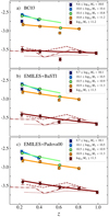 |
Fig. 1. Evolution of number density (Y-axis) of quiescent galaxies in ALHAMBRA with redshift (X-axis), for different stellar mass bins (see inner-panels). Coloured dots illustrate number densities when using a 1/Vmax formalism, whereas solid lines show the best fit to Eq. (1). From top to bottom, number densities obtained from BC03, EMILES+BaSTI, and EMILES+Padova00 SSP models (panels a, b, and c, respectively). Over-plotted, we show the evolution on the number density of massive quiescent galaxies, log10 M⋆ ≥ 11, with redshift from the previous work of Pozzetti et al. (2010, dashed line), Moresco et al. (2013, dotted line), and Moustakas et al. (2013, dash-dot line). In all cases, the number densities at the 0.5 < z < 0.7 bin are excluded from the fit as explained in the text. |
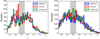 |
Fig. 2. Photometric-redshift distributions of quiescent (left panel) and star-forming (right panel) galaxies from the ALHAMBRA Gold catalogue down to 0.1 ≤ z ≤ 1.5. Distributions were obtained using the codes BPZ2.0, EAZY, and LePHARE (references in text). To guide the eye, the grey area encloses the redshift bin 0.5 ≤ z ≤ 0.7. |
The number density trends are quantified through a redshift-dependent, power-law function (solid lines in Fig. 1) of the form:
 (1)
(1)
For the different stellar mass bins, we provide the values ρ0 and γ that best fit our number density values in Table 2 (all the number density estimations at 0.5 ≤ z < 0.7 were removed from the fit). From Fig. 1, we summarise three remarkable results. Firstly, the number density evolution is well fitted by a power-law function (Eq. (1)). Secondly, the number density of quiescent galaxies is found to increase with cosmic time up to the present. Finally, at the low-mass end, quiescent galaxies have γ values that are compatible with a steeper evolution in number density with respect to the massive counterparts, meaning the appearance of low-mass quiescent galaxies is more prominent.
The least massive bin in our sample (9.6 ≤ log10 M⋆ < 10.0, dark blue dots in Fig. 1) greatly reflects the stellar mass range in which the stellar mass function of quiescent galaxies presents a local minimum or valley (Drory et al. 2009; Tomczak et al. 2014). However, owing to reasons of completeness we cannot establish the variation of its number density. At higher stellar mass, our fits suggest that the number density of quiescent galaxies ρN(z) grows on average by ∼52, 30, 20, 12% in the remaining mass bins, starting from the 10.0 ≤ log10 M⋆ < 10.4 interval, and between z = 0.4 and z = 0.2 (see Table 2). It is noticeable that the number densities retrieved with EMILES (see panels b and c in Fig. 1) show slightly larger variations than those obtained with the BC03 models (see panel a in Fig. 1), illustrating the dependence of ρN(z) on the SSP models adopted to retrieve stellar parameters.
Ilbert et al. (2013) reported that quiescent galaxies of log10 M⋆ > 11.2 dex suffer a rapid and efficient increase in number at 1 < z < 3. However, these galaxies do not exhibit prominent evolution since z ∼ 1, where the great number density variations of quenched galaxies are more focused on the less massive systems (a result also observed by e.g. Davidzon et al. 2013), in agreement with our results (see Table 2). Ferreras et al. (2005, 2009a) performed an analysis of morphologically-selected, early-type galaxies (ETGs) in the GOODS17 fields, finding a substantial difference between the co-moving number density of massive ETGs and their lower mass counterparts. Between z = 1 and z = 0.6, the number density of ETGs was found to increase only by a factor of 0.25 dex for log10 M⋆ > 11, and it was even compatible with no evolution at the most massive end (log10 M⋆ > 11.5, see also Ferreras et al. 2009b). Pozzetti et al. (2010) found that the number density evolution of quiescent galaxies (log10 M⋆ > 11) is not significant, with a variation ∼0.1 dex, since z ∼ 0.85 up to z ∼ 0.25; while in our work this variation is ∼0.12–0.25 dex. Moresco et al. (2013) claimed that the number of quiescent galaxies (log10 M⋆ ∼ 10.5) increases by ∼80% between z ∼ 0.65 and z ∼ 0.2, which is compatible with ours (60–75%), while the massive ones (log10 M⋆ > 11) were compatible with no evolution. With different selection criteria, Moustakas et al. (2013) found that the number of quiescent galaxies in the mass range 10.0 < log10 M⋆ < 10.5 increases by a 60 ± 20% fraction between z ∼ 0.6 and z ∼ 0.2; at 10.5 < log10 M⋆ < 11.0 the increase is around 40 ± 10% between z = 0.8 and z = 0.2; and for 11.0 < log10 M⋆ < 11.5 the increment is 20 ± 10% at 0.2 < z < 1.0. Using the same redshift range and stellar mass bins as Moustakas et al. (2013), we find number density variations of 90 ± 40%, 60 ± 20%, and 40 ± 20% using BC03 SSPs (and larger variations with EMILES), respectively. In Fig. 1, we illustrate the behaviour of the number density at the most massive bin, log10 M⋆ > 11.2. It should be noted that in our work, we cull dusty star-forming galaxies from the sample of quiescent galaxies via the MCDE, a procedure that differs with respect to the selections of previous studies.
On the other hand, previous studies, such as Cerulo et al. (2016, and references therein), claim that low-mass quiescent cluster galaxies at the faint end of the stellar mass function have not presented a remarkable evolution in number since z ∼ 1.5. However, the authors suggest that this is a consequence of the halo mass, which accelerates the building-up of the passive population of galaxies. In ALHAMBRA, which extends over six uncorrelated fields, we would expect the sample to be dominated in number by field galaxies, explaining why our results differ with respect to others defined in dense environments.
4. Stellar populations of quiescent galaxies since z∼ 1
This section presents the main results, namely the evolution of the stellar population properties of quiescent galaxies during the last 8 Gyr of cosmic time. With this aim, we build, for the first time, analytic PDFs of the properties of quiescent galaxies since z ∼ 1 (Sect. 4.1). Finally, we describe in detail the observed changes in the stellar content of quiescent galaxies, making use of the redshift-dependent PDFs of mass-weighted age (Sect. 4.2), metallicity (Sect. 4.3), and extinction (Sect. 4.4).
4.1. Probability distribution functions of stellar population parameters
Our sample contains quiescent galaxies covering a wide redshift range, noting that the derived uncertainties of the stellar population parameters have a significant dependence on redshift. Moreover, certain ranges of stellar-population parameters are intrinsically more subject to SED-fitting errors (see Fig. 11 in Díaz-García et al. 2015), usually related to well-known degeneracies amongst parameters (such as the age-metallicity degeneracy, Worthey 1994, 1999; Peletier 2013; Díaz-García et al. 2015). To illustrate this, the median of the age, metallicity, and extinction uncertainties obtained by MUFFIT and the ALHAMBRA data set is shown in Fig. 3. In our sample, quiescent galaxies at higher redshift exhibit lower age uncertainties (see panel a in Fig. 3). In fact, this behaviour was also observed using simulations (Díaz-García et al. 2015) and it is a consequence of the age range of SSP models at larger redshifts (they cannot be much larger than the age of the Universe) and because a wider wavelength range of the rest-frame near-UV regime is observed. On the other hand, metallicity and extinction uncertainties are larger at increasing redshift (see panels b and c in Fig. 3, respectively). Consequently, the uncertainties can modify the distributions of stellar population parameters in a redshift-dependent way. This behaviour hinders both a direct comparison amongst the distribution of the stellar-population parameters at different redshifts, as well as a precise reconstruction of the intrinsic distribution.
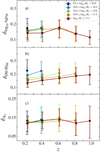 |
Fig. 3. Typical uncertainties of stellar population parameters of ALHAMBRA quiescent galaxies. From top to bottom, median of age, metallicity, and extinction uncertainties (panels a, b, and c, respectively) at different redshifts and stellar mass bins (see inner panel). Vertical bars enclose the 68% confidence level of the distribution of uncertainty values. |
We dealt with this issue by performing a maximum likelihood estimator (MLE) method to deconvolve uncertainty effects, and build PDFs of the involved stellar population properties of the quiescent galaxy population (not individual galaxies): mass-weighted ages, metallicities and extinctions. In particular, we adapted the MLE methodology developed by López-Sanjuan et al. (2014), also used in DG17, to deconvolve observational errors from observed distributions at different stellar mass ranges. In practise, this technique aids in recovering the intrinsic scatter of stellar population distributions from the observed ones, which are affected by uncertainties. We therefore constrained the most likely set of parameter values to maximise the probability distributions. As a result, we obtain a set of functional and analytical distributions fitted by log-normal functions, and re-normalise them with their number densities (see Sect. 3). For further details of the whole process, we refer interested readers to Appendix A.
It should be noted that, as mentioned in Appendix A, we did not provide the redshift-dependent PDFs for quiescent galaxies at log10 M⋆ < 10.1, because the reliability of the MLE method is compromised, owing to the low number of sources. Instead, and only for the least massive case, we applied the MLE method assuming no redshift dependence of the PDF parameters (i.e. μ2 = μ1 = σ2 = σ1 = 0, details in Appendix A) in order to set the average values of the median and width of the stellar population parameter distributions at 0.1 ≤ z < 0.3.
In the following, to detail the evolution of the PDFs with redshift, we focus on the evolution of their medians and widths. For this work, we defined the width of a PDF as the difference between the 84th and 16th percentiles. Note that the width at this point is not a result of uncertainty effects, but the intrinsic dispersion of stellar population properties. The main results of this section, that is, the medians and widths of the PDFs of quiescent galaxies can be found in Figs. 4–6 (showing the mass-weighted age and formation epoch, metallicity, and extinction, respectively). As shown in these figures, the PDF parameters evolve with redshift (X-axis in the figures) and depend on the stellar mass range (coloured lines, see insets). It should be noted that the SSP sets of BC03 (first column in figures), EMILES with both BaSTI (second column), and Padova00 (third column) isochrones are included to explore potential systematics due to the use of different population synthesis models.
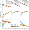 |
Fig. 4. Evolution of mass-weighted age and formation epoch PDFs of quiescent population along cosmic time for different stellar mass bins. Panels a–c and panels d–f: illustrate the evolution of the medians of mass-weighted age and formation epoch PDFs, respectively, whereas panels g–i show the widths of the mass-weighted age PDFs. From left to right, results obtained using the SSP models of BC03 (panels a, d, and g), EMILES with BaSTI isochrones (panels b, e, and h), and EMILES with the Padova00 ones (panels c, f, and i). The shaded regions enclose the 1σ uncertainties of both parameters. The grey region limits the age of the Universe at any redshift. The square-shaped markers illustrate the average median and width assuming for the MLE deconvolution μ2 = μ1 = σ2 = σ1 = 0. |
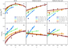 |
Fig. 5. Evolution of mass-weighted metallicity PDFs of quiescent population along cosmic time for different stellar mass bins. Panels a–c: illustrate the evolution of the medians of mass-weighted metallicity PDFs, whereas panels g–i show the widths of the mass-weighted metallicity PDFs. From left to right, results obtained using the SSP models of BC03 (panels a and d), EMILES with BaSTI isochrones (panels b and e), and EMILES with the Padova00 ones (panels c and f). The shaded regions enclose the 1σ uncertainties of both parameters. The grey region limits the age of the Universe at any redshift. The square-shaped markers illustrate the average median and width assuming for the MLE deconvolution μ2 = μ1 = σ2 = σ1 = 0. |
4.2. Ages and formation epochs
Our results show that the mass-weighted age and formation epoch PDFs are correlated with the stellar mass of quiescent galaxies, showing systematic variations that depend on the stellar mass (see panels a to f in Fig. 4). In good agreement with the downsizing scenario, more massive quiescent galaxies feature a larger stellar content in old stars with respect to the lower mass systems, which are preferentially formed at more recent epochs. The median ages (see panels a–c in Fig. 4) of the quiescent population present older stellar populations at lower redshifts independently of the stellar mass bin, as to be expected in passive or quenched systems. Nevertheless, the median of the formation epoch PDFs of quiescent galaxies (panels d–f in Fig. 4) exhibits a continuous and general decrement at lower redshifts for all the stellar masses and SSP models used in this work, especially for BC03 (see panel d in Fig. 4), which is not compatible with pure passive evolution. For the most massive case, log10 M⋆ ≥ 11.2, the formation epoch at z ∼ 1.0 is ∼12–13 Gyr (equivalent to a formation redshift of zf ∼ 4.5–6), whereas at z = 0.2 the median formation epoch decreases to ∼9–11 Gyr (i.e. corresponding to a formation redshift of zf ∼ 1.5–3). At lower stellar masses, the variation of the formation epochs is more pronounced. It is worth mentioning that the mass-weighted ages retrieved from BC03 models are younger than the ones obtained for EMILES with BaSTI (0.15–0.2 dex or 2–3 Gyr) and Padova00 (0.05–0.10 dex or 1.5–2 Gyr) isochrones. It is of note that the BaSTI isochrones provide ages older than those from Padova00, as the BaSTI isochrones are bluer than the Padova00 ones (Vazdekis et al. 2016).
The width of the mass-weighted age and formation epoch PDFs are roughly the same (see panels g–i in Fig. 4). These are fairly constrained in the range 0.1–0.2 dex (∼1–2 Gyr). Using EMILES and BaSTI isochrones, the width of the mass-weighted age PDFs does not present a great dependence with stellar mass. In the case of EMILES+Padova00, we retrieved the same trend, although the PDFs are slightly wider (see panels g–i in Fig. 4). Our results point out that the evolution with redshift of the widths of the age and formation epoch PDFs is mild. In fact, for EMILES and BaSTI there is no evidence of evolution with redshift. Only for BC03 at log10 M⋆ < 10.8, the widths of the mass-weighted age and formation epoch PDFs decrease at larger cosmic times, with values in the range of 0.06–0.18 dex (or ∼1–2.5 Gyr). For EMILES, we do not find that the evolution with redshift of the widths of mass-weighted age and formation epoch PDFs strongly depends on mass.
4.3. Evolution of metal content
We turn now to the median and width of the mass-weighted metallicity PDFs (see panels a–c in Fig. 5). From the results shown in panels a–f of Fig. 5, we infer a correlation between stellar mass and metallicity. At any redshift, the higher the galaxy mass, the larger the metal content. In general, quiescent galaxies present median metallicities around solar and super-solar values. Only the least massive galaxies at the lowest redshift in our sample exhibit sub-solar metallicities on average. The median of the mass-weighted metallicity PDF also exhibits a dependence with redshift (see panels a–c in Fig. 5). When using EMILES SSP models (panels b and c in Fig. 5), there is evidence of a decrease in the median of the mass-weighted metallicity PDFs of quiescent galaxies since z ∼ 1. This behaviour is intrinsic to the whole quiescent population and independent of stellar mass. In the most massive bin, log10 M⋆ > 11.3, this decrease amounts to ![Mathematical equation: $ \Delta \mathrm{[M/H]}_\mathrm{M}^{50\mathrm{th}} \sim 0.2 $](/articles/aa/full_html/2019/11/aa32882-18/aa32882-18-eq2.gif) dex for EMILES and BaSTI isochrones, whereas for the Padova00 ones, the variation is
dex for EMILES and BaSTI isochrones, whereas for the Padova00 ones, the variation is ![Mathematical equation: $ \Delta \mathrm{[M/H]}_\mathrm{M}^{50\mathrm{th}} \sim 0.1 $](/articles/aa/full_html/2019/11/aa32882-18/aa32882-18-eq3.gif) dex. At decreasing stellar mass, this decrease is steeper, suggesting that the slope of the MZR for quiescent galaxies varies with redshift. For BC03 SSP models (see panel a in Fig. 5) the evolution of the median metallicity exhibits a maximum value at z ∼ 0.5–0.6. A decrease of the median metallicity at earlier cosmic times is also present, but only since z ∼ 0.6, noting that the uncertainty is
dex. At decreasing stellar mass, this decrease is steeper, suggesting that the slope of the MZR for quiescent galaxies varies with redshift. For BC03 SSP models (see panel a in Fig. 5) the evolution of the median metallicity exhibits a maximum value at z ∼ 0.5–0.6. A decrease of the median metallicity at earlier cosmic times is also present, but only since z ∼ 0.6, noting that the uncertainty is ![Mathematical equation: $ \Delta \mathrm{[M/H]}_\mathrm{M}^{50\mathrm{th}} \sim 0.2 $](/articles/aa/full_html/2019/11/aa32882-18/aa32882-18-eq4.gif) dex. Interestingly, this peak matches the redshift range where we report a lack of quiescent galaxies in ALHAMBRA owing to cosmic variance (see Sect. 3 and Fig. 1), a result that appears more prominent with BC03 models. In light of Fig. 5 (panels a–c), there are also quantitative discrepancies between metallicity predictions from the use of different SSP models, and these are more striking for metallicity than for the rest of stellar population properties. In brief, BC03 models predict quiescent galaxies that are typically richer in metals than those in EMILES models at any redshift, where BaSTI isochrones provide larger metallicities than the Padova00 ones.
dex. Interestingly, this peak matches the redshift range where we report a lack of quiescent galaxies in ALHAMBRA owing to cosmic variance (see Sect. 3 and Fig. 1), a result that appears more prominent with BC03 models. In light of Fig. 5 (panels a–c), there are also quantitative discrepancies between metallicity predictions from the use of different SSP models, and these are more striking for metallicity than for the rest of stellar population properties. In brief, BC03 models predict quiescent galaxies that are typically richer in metals than those in EMILES models at any redshift, where BaSTI isochrones provide larger metallicities than the Padova00 ones.
Regarding the width of the metallicity PDFs (panels d–f in Fig. 5), there is evidence that the metallicity distributions of quiescent galaxies are typically wider at lower mass, whereas the distribution is narrower at higher stellar mass. The less massive bins (log10 M⋆ < 10.9) present widths in the range of ω[M/H]M ∼ 0.3–0.5 dex up to z ∼ 0.5; whereas for log10 M⋆ ≥ 10.9, these are below ω[M/H]M ≲ 0.3 dex. Nevertheless, for quiescent galaxies of log10 M⋆ ≥ 10.9, there are discrepancies down to 0.2 dex between the widths of the mass-weighted metallicity PDFs retrieved using BC03 and EMILES SSP models. While for BC03, these present a more relevant evolution with redshift; for EMILES they present a roughly constant width of ω[M/H]M ∼ 0.3 dex, with a slight redshift dependence. In addition, BC03-derived metallicities show that the evolution of the metallicity PDF widths is independent of the stellar mass of quiescent galaxies, whereas those derived with EMILES suggest a dependence with stellar mass.
4.4. Extinction in the quiescent population
Overall, the extinction PDFs of quiescent galaxies derived in this research (see panels a–f in Fig. 6) show predominant low values (AV ≲ 0.6) irrespectively of stellar mass or redshift. Indeed, the median of the extinction PDFs at all stellar masses and redshifts does not exceed  .
.
From panels a–c in Fig. 6, we infer a very subtle relation between the stellar mass and dust extinction of quiescent galaxies with differences  when using BC03 SSP models. For EMILES, we do not appreciate significant differences in the median values of the extinction PDFs amongst the stellar mass bins (see panels b and c in Fig. 6), where all the values retrieved are compatible at a 1σ confidence level for both BaSTI and Padova00 results. Independently of the SSP model set used in this work, the median of extinction PDFs vary around
  –0.30 up to z = 1.1. We also find that there is a subtle increment of extinction in the lower-mass bins (log10 M⋆ ≤ 10.8) at decreasing redshift. On the other hand, quiescent galaxies with log10 M⋆ ≥ 10.8 show that the median extinction remains constant
  for EMILES and in the range of
  –0.30 for BC03 models.
Estimates from both BC03 and EMILES point out that there may be mild discrepancies between the widths of the extinction PDFs at different stellar masses (see panels d–f in Fig. 6). In any case, these discrepancies amount to width differences below 0.1. The lower the stellar mass, the larger the width of the PDF. At decreasing redshift the extinction PDFs get narrower across all stellar masses, where less massive quiescent galaxies present broader probability distributions. Note that for the BC03-derived results at 0.1 ≤ z < 0.2 and log10 M⋆ ≥ 11.2, the assumption of linearity for σint(z) and μ(z) in the extinction case is too strict, so we imposed σint(0.1 ≤ z < 0.2)=σint(z = 0.2) = 0.14 ± 0.03 and μ(0.1 ≤ z < 0.2)=μ(z = 0.2)= − 1.30 ± 0.07 (details in Appendix A.1).
4.5. Constraints on the SFH
The different SFH assumptions adopted in the construction of composite models of stellar populations may have a potential impact on the results shown above. We studied these effects, repeating the full analysis with new sets of composite models applying alternative SFH constraints. For this work, we explore the following assumptions on the SFH: (i) constant values of extinction for all quiescent galaxies at any redshift and stellar mass; (ii) fixed solar metallicity; (iii) closed-box enrichment of metals, meaning the young component in the mixture of the two SSP models of MUFFIT has to be more metal-rich than the old one; (iv) SSP mixtures with the same metallicity for the old and young components; (v) infall of metal-poor, cold gas from the cosmic web, namely the young component in the mixture of SSPs is more metal poor than the old component; (vi) quiescent galaxies exhibit a constant MZR with cosmic time, matching the one in the nearby Universe (this test is only performed for EMILES with BaSTI isochrones).
After studying the impact of these constraints on the stellar population parameters of quiescent galaxies and PDFs, we firstly find that none of these SFH assumptions alter our main conclusions, namely the evolution of quiescent galaxies is not compatible with a passive evolution and there is a continuous decrease in metallicity (trivially excluding the fixed solar metallicity assumption above) since z ∼ 1. Secondly, SFH constraints introduce non-negligible systematics that quantitatively alter the age, metallicity, and extinction. Finally, we find that constraints on the SFH are a source of quantitative uncertainties that can have a larger impact than the “basic” uncertainties obtained in the determination of the stellar population parameters.
5. A global view on the evolution of quiescent galaxies since z∼ 1
The PDFs of mass-weighted age, metallicity, and dust extinction of quiescent galaxies since z ∼ 1 have constrained the evolution of these systems during the last 8 Gyr of cosmic time in an unprecedented way. Thanks to the statistical deconvolution of uncertainty effects (MLE method, details in Appendix A), and to the large and mass-complete set used here (∼8500 galaxies), it is possible to explore the evolution of quiescent galaxies as a whole. In particular, the intrinsic dispersions of the PDFs constitute new observables to constrain the evolution of quiescent galaxies.
This work presents evidence suggesting that the age evolution of quiescent galaxies departs from a passive scenario, showing milder ageing on average. This conclusion is obtained even when assuming different constraints on the SFHs during the MUFFIT analysis (Sect. 4.5). Moreover, we find evidence for a slight decrease of the median of the metallicity PDF (0.1–0.2 dex) of quiescent galaxies since z ∼ 0.6–1.1 (BC03 and EMILES, respectively), consistently obtained under most of the adopted SFHs, and constitutes one of the most striking results of this work. Both a steeper MZR at larger cosmic time and the continuous decrease of the median metallicity with time additionally support that quiescent galaxies are continuously modifying their stellar content.
All these results are in conflict with strict passive evolution. Two alternative scenarios are discussed here to reconcile observations on the evolution of quiescent galaxies, as well as establishing the role of the progenitor bias:
-
(i)
Mergers. The inclusion of new stars, formed ex-situ from less massive systems may be a potential mechanism to alter the stellar content of galaxies (see e.g. Ferreras et al. 2005; Croton et al. 2006; Khochfar & Silk 2006; Hopkins et al. 2008; Kaviraj et al. 2008; Ferreras et al. 2009a,c, 2014; Hopkins et al. 2009; Rogers et al. 2009; Sánchez-Blázquez et al. 2009b; van der Wel et al. 2009; Díaz-García et al. 2013; López-Sanjuan et al. 2013; Skelton et al. 2012). In this case, the number of mergers involving quiescent galaxies is key to discerning whether this mechanism can match the observed non-passive evolution.
-
(ii)
Remnants of star formation or “frosting” (a term first introduced by Trager et al. 2000). Clouds of gas inside the galaxy or the infall of new gas from the cosmic web can originate new stellar populations with different properties than those already present in the galaxy (Ferreras & Silk 2000; Trager et al. 2000; Schiavon et al. 2006; Kaviraj et al. 2007; Rogers et al. 2007; Schiminovich et al. 2007; Serra & Trager 2007; Somerville et al. 2008; Ferreras et al. 2009c; Rogers et al. 2009; Lonoce et al. 2014; Vazdekis et al. 2016).
-
(iii)
The progenitor bias (van Dokkum & Franx 2001). Quiescent galaxies at high redshift provide a biased set with respect to their nearby counterparts, and therefore, not all the progenitors of the low redshift sample are included in the analysis (see also Valentinuzzi et al. 2010; Carollo et al. 2013; Belli et al. 2015). Indeed, the generalised increase in the number of quiescent galaxies since z ∼ 1 motivates the inclusion of the progenitor bias in the discussion.
Below, we discuss and detail the likely effects of mergers and frosting on the stellar content of quiescent galaxies, more precisely on age (Sect. 5.1), metallicity (Sect. 5.2), and extinction (Sect. 5.3).
5.1. Ages of quiescent galaxies
A galaxy undergoing natural ageing would exhibit a constant formation epoch with cosmic time. Otherwise, we would conclude that the population of quiescent galaxies is being altered. Mergers and frosting may have a relevant role on the typical ages of quiescent galaxies because these processes introduce new stars in the stellar content of quiescent galaxies. In fact, these mechanisms can act in parallel, increasing their mutual effects. On the other hand, part of the progenitors of low-redshift quiescent galaxies are not included in our sample, and their stellar content can differ with respect to high-redshift quiescent galaxies. The consequences of each of these mechanisms and the progenitor bias mentioned above are discussed in the same order in which they were presented:
-
(i)
Less massive systems are expected to contain younger stellar populations due to the age–mass relation (see e.g. Gallazzi et al. 2005; Thomas et al. 2005; Peng et al. 2015), in qualitative agreement with the downsizing scenario. Hence these systems are potential contributors to “slowing down” the ageing of quiescent galaxies when they are accreted via mergers.
-
(ii)
The inclusion of new (and in-situ) stars would easily explain why the evolution of these galaxies departs from passiveness. However, frosting is needed to affect the whole quiescent population to be a reliable mechanism.
-
(iii)
Part of the progenitors of the nearby quiescent galaxies from ALHAMBRA were star-forming galaxies in the high redshift bins explored in this work, that is, these progenitors were still forming new stars at that epoch. Consequently, galaxies quenching their star formation at more recent epochs will contain younger stellar populations. Hereby, the samples of high redshift quiescent galaxies are biased to the older parts of the age PDFs at lower redshift. This result would partly explain why the median ages of quiescent galaxies do not vary passively.
5.2. Metallicities of quiescent galaxies
The evolution of the mass-weighted metallicity PDFs contributes an extra indication, pointing out that some of the mechanisms discussed above may be altering the typical stellar population parameters of quiescent galaxies. The consequences, listed separately for each of the scenarios considered, would be the following:
-
(i)
Mergers with less massive systems can contribute to the observed variation of the global metallicity, as less massive systems host metal-poorer populations with respect to the more massive galaxy in the pair, owing to the stellar mass-metallicity relation (see e.g. Peng et al. 2015; Jørgensen et al. 2017). Again, the number of mergers would determine whether this mechanism is capable of altering the median of the mass-weighted metallicity PDF.
-
(ii)
A priori, frosting would not explain a decrease of the global metallicity in a monolithic collapse. However, in the chemo-evolutionary population synthesis model by Vazdekis et al. (1996, which does not take into account any interchange of matter with the neighbourhood, also known as a closed-box model), the global metallicity of a galaxy may decrease at a certain cosmic time. Owing to a very intense star formation, the available gas decreases very rapidly and the enrichment of metals quickly asymptotes to the net yield. Then, all the available gas mostly comes from the numerous oldest low-metallicity stars, which is less processed, producing new stellar populations that can reduce the metallicity to around 0.2 dex at ∼10 Gyr after the initial star formation. For bottom heavy IMFs, this effect is even more prominent.
-
(iii)
If the progenitors of low redshift quiescent galaxies are biased at high redshift because they are still assembling their stellar content, the progenitor bias would only affect the results in the direction of more metal-poor metallicity. In fact, the evolution in number density of quiescent galaxies since z ∼ 1 is more remarkable at decreasing stellar mass. Therefore, the progenitors of our sample of quiescent galaxies are likely more biased at lower masses and the metallicities would be more affected by the progenitor bias, that is presenting larger variations in metallicity, as is observed in this work.
5.3. Extinctions of quiescent galaxies
The extinction of quiescent galaxies presented in this paper are well constrained below AV < 0.6 and they do not present large variations with cosmic time. Indeed, extinction is roughly constant (AV ∼ 0.2) for EMILES models. Consequently, the effects of mergers, frosting, and the progenitor bias may be less remarkable here than for ages and metallicities (see Sects. 5.1 and 5.2), and they can even cancel each other. We would expect the following impact on the extinction PDFs:
-
(i)
Mergers between quiescent and star-forming galaxies (with the latter expected to feature larger extinction) will increase the overall extinction of the resulting galaxy. The merger orbit, as well as the distribution of dust in the progenitors would drive how the global extinction of the final galaxy is affected.
-
(ii)
Concerning frosting, we would not expect that low levels of in-situ star formation can alter typical extinction values in quiescent galaxies, which are expected to have low reserves of available gas and where current star formation processes are not significant yet.
-
(iii)
Since star-forming galaxies are typically more reddened by dust than quiescent ones, our sample of quiescent galaxies at high redshift can be biased to lower extinctions. However, the mechanism responsible for shutting down the star formation is still unknown, as well as the typical extinction of galaxies quenching their star formation. In fact, the evolution of extinction in star forming galaxies is unclear, and the quenching mechanism can also be tightly related to it (e.g. sudden removal of gas, “strangulation”, or heating of a galaxy’s gas by AGN, Silk & Rees 1998; Balogh et al. 2000; Dekel & Birnboim 2006; Hopkins et al. 2006; Nandra et al. 2007; Bundy et al. 2008; Di Matteo et al. 2008; Diamond-Stanic et al. 2012; Peng et al. 2015).
In general, mergers and frosting can potentially contribute to modifying the width of the mass-weighted age, metallicity, and extinction PDFs of quiescent galaxies, which constitutes an additional hint towards the variation of their stellar content. In fact, a unique mechanism would not be able to produce all the changes revealed in this work, but rather a simultaneous combination of merger and frosting may be a more realistic scenario. Independently of the impact of each of the mechanisms mentioned above, any evolution in the widths of the stellar population PDFs, or intrinsic scatter, requires either a non-passive evolution or an external mechanism acting on the stellar content of quiescent galaxies. In addition, we have to take into account that part of the PDF evolution may be a consequence of a biased sample as we only focus on the stellar content of quiescent galaxies over a wide redshift range (i.e. the progenitor bias).
6. Comparison with previous studies
The evolution of the stellar populations of quiescent galaxies has been mainly tackled using spectroscopic data. In fact, these kinds of studies usually require an analysis based on stacked spectra, which does not allow us to determine the intrinsic dispersion of the stellar population distributions. In this section and whenever possible, we compare the ages and metallicities retrieved in this research using the ALHAMBRA data with those from previous studies (see Table 3 for further details). As the quiescent galaxies from ALHAMBRA comprise a wide range in cosmic time, we structured this section according to the redshift range explored (Sects. 6.1–6.3).
Brief description of previous studies trying to constrain stellar population parameters of quiescent galaxies at intermediate redshift.
6.1. Ages and metallicities of quiescent galaxies in the nearby Universe
Aimed at exploring the mechanisms responsible for quenching galaxies, Peng et al. (2015) studied both the metallicity- and age-stellar mass relations of quiescent galaxies at 0.05 ≤ z ≤ 0.085. The quiescent sample was composed of 22 618 galaxy spectra from SDSS18, where ages and metallicities were measured by a multiple fit to age and metallicity-sensitive indices (see also Gallazzi et al. 2005). After comparing the age estimations provided by MUFFIT and BC03 (or EMILES+BaSTI) SSP models with the ones from Peng et al. (2015), the latter are ∼1.5 Gyr older (or younger) with a similar correlation between age and stellar mass for log10 M⋆ ≥ 10 (see panels a and b in Fig. 7, respectively). The EMILES+Padova00 age-stellar mass relation is steeper, but the range of ages for quiescent galaxies is qualitatively the same as the one provided by Peng et al. (2015, see panel c in Fig. 7). Regarding metallicity, there is a shift of ∼ − 0.2 dex between our BC03 and EMILES+BaSTI values and those provided by Peng et al. (2015, see panel d and e in Fig. 7). For the Padova00 models, at the lowest metallicity values, this shift is even larger (Δ[Fe/H] ∼ −0.3 dex). Although if we account for the SDSS aperture effects (0.15–0.2 dex, Gallazzi et al. 2005), our metallicity predictions agree with those provided by Peng et al. (2015).
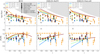 |
Fig. 7. Comparison of ages (panels a, b, and c) and metallicities (panels d, e, and f) of quiescent galaxies from several previous studies and our results from ALHAMBRA at redshift range 0 < z < 1.2. From left to right, the median mass-weighted ages and metallicities retrieved using MUFFIT (solid lines) and BC03 (panels a and d), EMILES with BaSTI (panels b and e), and Padova00 isochrones (panels c and f), respectively. The ages and metallicities retrieved from other work are colour-coded in concordance with their proximity to the stellar mass bins of our quiescent sample (see inset). Dashed orange lines illustrate the average age and metallicity in galaxy clusters obtained by Jørgensen et al. (2017). The grey region limits the Universe age. |
6.2. Quiescent galaxies at intermediate redshifts
Our sample of quiescent galaxies is expected to be dominated by field galaxies. However, galaxies in dense environments may present systematic differences in their stellar contents with respect to field samples (e.g. Sánchez-Blázquez et al. 2003; Eisenstein et al. 2003; Thomas et al. 2005, 2010; Trager et al. 2008). For this reason we distinguish between spectroscopic studies that include field quiescent galaxies (Sect. 6.2.1) and those in clusters (Sect. 6.2.2) to compare with our results.
6.2.1. Stellar content of field quiescent galaxies
The spectroscopic study of Schiavon et al. (2006) also revealed that the ages of RS galaxies at z ∼ 0.9 are not compatible with a passive evolution. More precisely, the authors found that RS galaxies from the DEEP2 surveys (Davis et al. 2003) present luminosity-weighted SSP ages around ∼1.5 Gyr. These ages are significantly younger than the ones obtained by MUFFIT for quiescent galaxies (see panels a–c in Fig. 7, mass-weighted ages of 5 Gyr). Nevertheless, this qualitative difference is in part explained by the use of both index-index diagrams (e.g. luminosity-weighted ages) and simple stellar population models to estimate ages. Regarding metallicities, there is a reasonable agreement between the iron abundances of Schiavon et al. (2006; [Fe/H] = 0.0–0.3 dex) and the ones by MUFFIT (0.12, 0.13, −0.04 dex for BC03, BaSTI, and Padova00; see panels d–f in Fig. 7). Finally, Schiavon et al. (2006) also concluded that either RS galaxies experienced a continuous, low-level star formation, or there is an inclusion of new galaxies with younger stellar populations, in other words, frosting and the progenitor bias (e.g. Trager et al. 2000; Bell et al. 2004; Faber et al. 2007).
Ferreras et al. (2009c) used low-resolution slitless grism optical spectra from the Hubble Space Telescope (HST) Advanced Camera Survey to constrain the stellar populations of a sample of visually-selected ETGs at 0.4 < z < 1.3. Overall, the authors found a strong correlation between stellar age and mass at intermediate redshift where the age spread was roughly constant at around ∼1 Gyr. Ferreras et al. (2009c) also divided their morphologically selected sample into red and blue galaxies. For a fair comparison, we selected all the red ETGs at 0.4 < z < 1.3 and 10.6 < log10 M⋆ < 11.4 to create a representative sub-sample to compare with our predictions (a ∼90% fraction of ETGs at this mass range and redshift are quiescent galaxies, see Moresco et al. 2013). Red ETGs exhibit ages close to passive evolution, hence showing a better agreement with our predictions using EMILES+BaSTI SSP models and larger discrepancies with the BC03 models (see panels a–c in Fig. 7). Regarding metallicity, Ferreras et al. (2009c) present more metal-poor populations than our predictions, as expected from the use of a chemical enrichment model of stellar populations in comparison with other composite models (e.g. τ-models or two-burst models; in any case compatible with a χ2 ∼ 1 for all the composite models, see Ferreras et al. 2009c). However, we cannot state a clear decrease in metallicity at 0.4 < z < 1.3 for the galaxies from Ferreras et al. (2009c).
At a similar redshift range, Choi et al. (2014) analysed the stellar populations of quiescent galaxies up to z < 0.7. They computed SSP equivalent ages and abundances of elements by stacked spectra. Choi et al. (2014) found that quiescent galaxies are older at lower redshift and compatible with both a downsizing scenario and a composed passive evolution. Regarding [Fe/H], unlike our predictions, the authors do not clearly retrieve either the MZR at lower redshift or a metallicity evolution with redshift. In addition, they state that the metallicity can be potentially affected by aperture effects (an excess of ≲0.1 dex at the lowest redshifts). In fact, the metallicity decrease obtained in our work is ≲0.15 dex since z = 0.7, that is, similar to the aperture bias reported by Choi et al. (2014).
Using a multiple fit to age- and metallicity-sensitive absorption features, Gallazzi et al. (2014) explored the ages and metallicities of 33 quiescent galaxies at z ∼ 0.7 with stellar mass M⋆ > 3 × 10¹⁰ M⊙. Gallazzi et al. (2014) found that ages of quiescent galaxies at z ∼ 0.7 are ∼2 Gyr younger than those obtained with a similar methodology at low-redshift (Gallazzi et al. 2005), that is, less than that predicted by a passively evolving assumption. We find that the mass-weighted ages of MUFFIT+BC03 are in good agreement with those provided by Gallazzi et al. (2014, panel a in Fig. 7). However, we obtain larger metallicities of Δ[Fe/H] ∼ 0.1 dex (see panel d in Fig. 7). For EMILES models, the ages provided by MUFFIT are ∼1.5 Gyr older (see panels b and c in Fig. 7). For BaSTI isochrones the agreement with metallicity is remarkable, mostly at the highest stellar mass bin.
Making use of spectroscopic data from the 3D-HST survey, Fumagalli et al. (2016) estimated the ages of UVJ quiescent galaxies at 0.5 < z < 2.0. Only the most massive galaxies (log10 M⋆ > 10.8) were selected in order to stack all the spectra in three redshift bins. As a result, the ages of quiescent galaxies present a large spread in age due to the use of different model sets, although typically below half of the age of the Universe. Our analysis at the same redshift ranges yields older mass-weighted ages. It is remarkable that the extrapolation at z = 1.25 of the mass-weighted ages (BC03 and EMILES) also match with the ages derived by Fumagalli et al. (2016) and BC03 models (see panel a in Fig. 7). It is worth mentioning that Fumagalli et al. (2016) only adopt solar metallicity models. This constraint may introduce substantial systematics in the retrieved ages that can lead to passive evolution of the stellar content.
6.2.2. Quiescent galaxies in clusters up to intermediate redshifts
The stellar population properties of RS galaxies in clusters and groups at 0.4 < z < 0.8 were studied by Sánchez-Blázquez et al. (2009a). The authors found that quiescent galaxies have older ages at lower redshift (see panels a–c in Fig. 7), which were compatible with a passive evolution at a 1σ uncertainty level (formation redshift zf > 1.4). Interestingly, the most massive galaxies in Sánchez-Blázquez et al. (2009a) exhibit hints for a decrease in metallicity at lower redshift, which would be in qualitative agreement with our results (see panels d–f in Fig. 7). Regarding the less massive systems, they showed neither age nor metallicity evolution within the errors. Overall, they concluded that massive red galaxies are compatible with passive evolution, whereas the low mass systems either need a continuous level of star formation to maintain a constant age or the RS is in a continuous build-up adding new stars. Nevertheless, as commented above, the stellar population properties of galaxies in clusters may slightly differ with respect to those in the field (e.g. Sánchez-Blázquez et al. 2003; Eisenstein et al. 2003; Thomas et al. 2005, 2010; Trager et al. 2008).
Jørgensen et al. (2017) analysed the stellar populations of passive galaxies in seven massive clusters at 0.2 < z < 0.9 (see also Jørgensen et al. 2005; Chiboucas et al. 2009; Jørgensen & Chiboucas 2013). This study comprises multiple absorption-line strengths to interpret ages, metallicities, and abundance ratios [α/Fe] of composite spectra using the models of Thomas et al. (2011). It is worth noting that the age of their passive galaxies does not present a correlation with velocity dispersion. However, there is a steep relation between velocity dispersion and metallicity, which is constant at any redshift. This fact reflects that the MZR is also observed up to z ∼ 1, but differs from our results in that the MZR does not depend on redshift (see panels d–f in Fig. 7). Jørgensen et al. (2017) discuss that their local reference sample includes galaxies that are too young to be the descendant of the passive galaxies at intermediate redshift if only passive evolution is at work. They also reveal intrinsic scatter on the age and metallicity of 0.08–0.15 dex. The scatter in age agrees with our results, but it is lower than ours for metallicity. However, the authors used velocity dispersions instead of stellar mass to build their relations, which would explain these discrepancies (Trager et al. 2000; Gallazzi et al. 2006; Graves & Faber 2010; Cappellari et al. 2013).
6.3. Spectroscopic quiescent galaxies at z≳ 1
By use of Keck LRIS (Low Resolution Imaging Spectrometer) spectra and photometric data, Belli et al. (2015) retrieved the ages, metallicities, and extinctions of 51 quiescent galaxies at 1 < z < 1.6. In this sample, there are twelve galaxies at 1.0 < z < 1.12 with median stellar mass equal to log10 M⋆ ∼ 11.1). The median age, metallicity, and extinction of this sub-sample is 2.3 Gyr, −0.1 dex, and 0.36, respectively. At the redshift upper-limit, MUFFIT suggests that massive quiescent galaxies (10.8 ≤ log10 M⋆ < 11.2) exhibit a median age of ∼4.2 Gyr, [Fe/H] = −0.05, 0.0, and 0.18 dex (BC03, EMILES+Padova00, and EMILES+BaSTI, respectively; see panels d–f in Fig. 7), and extinctions of AV ∼ 0.2. Belli et al. (2015) assumed metallicities around solar values, which would partly explain the discrepancies between ages and extinctions owing to colour degeneracies.
Making use of 171 quiescent galaxies at 1.4 < z < 2.2 from the 3D-HST grism survey (Brammer et al. 2012), Whitaker et al. (2013) explore the stellar content of quiescent galaxies via stacked spectra. The authors found that there are prominent absorption features in the G-band and some metal lines, indicative of evolved stellar populations with an average age ranging from 0.9 to 1.6 Gyr. However, the authors also found Hβ in emission as well as [O II] in the residuals when subtracting the best-fit model. This would indicate a presence of residual star formation, or even the presence of an AGN.
In summary, there is a general consensus regarding the evolution scenario since z ∼ 1 that is in good agreement with our results, whereby quiescent galaxies get older with cosmic time independently of their stellar mass. In addition, the downsizing scenario is well reproduced by several of the studies in this section, as well as the results obtained by MUFFIT using the ALHAMBRA data set and different sets of SSP models (BC03 and EMILES). Despite the good agreement amongst the studies shown above, there is a large spread of the stellar ages that are strongly related to the use of different techniques, stellar population models, and SFH assumptions. Concerning metallicity, there are fewer measurements, but most results point out that quiescent galaxies have around solar and super-solar metallicities, with hints that the MZR is already in place at earlier epochs. The difficulty of disentangling the evolution with redshift of the metal content in quiescent galaxies is, primarily, caused by the fact that in these galaxies this evolution is expected to be mild (∼0.1 dex), as the bulk of the star formation must have happened at higher redshift.
7. Summary and conclusions
By means of the catalogue of galaxies published by Díaz-García et al. (2019a), we selected all the galaxies classified as quiescent via the dust-corrected stellar MCDE. This catalogue is complete in stellar mass and in magnitude down to I = 23 and it contains ∼8500 quiescent galaxies with stellar population properties obtained at redshift 0.1 ≤ z ≤ 1.1. This catalogue provides stellar population parameters such as mass- and luminosity-weighted ages and metallicities, stellar masses, extinctions, photo-z, rest-frame luminosities, colours corrected for extinction, and uncertainties of the parameters. These parameters were computed through the multi-filter fitting tool for stellar population diagnostics MUFFIT (Díaz-García et al. 2015), only using the photometric data from the ALHAMBRA survey, and the SSP models of Bruzual & Charlot (2003) and EMILES (including the two sets of isochrones of BaSTI and Padova00).
We explored the co-moving number density of quiescent galaxies at 0.1 ≤ z ≤ 1.1 and find an increasing number of quiescent galaxies from high redshift to the present time. The evolution of the number densities is well reproduced by a power-law function (as proposed by Moustakas et al. 2013). We find that the increase in number density for less massive quiescent galaxies is higher than for the massive case (∼52% and 12% fraction between z = 0.4 and z = 0.2 for 10 ≤ log10 M⋆ < 10.4 and log10 M⋆ ≥ 11.2, respectively). The above numbers agree within a downsizing picture in which low mass galaxies were formed in more recent epochs than the massive ones.
We also studied the evolution of the stellar population parameters of quiescent galaxies since z = 1.1 based on the results provided by MUFFIT and ALHAMBRA photometry. We construct, for the first time, the probability distribution functions (PDF) of mass-weighted age and formation epoch, metallicity, and extinction during the last 8 Gyr, using a maximum likelihood estimator in order to deconvolve the uncertainty effects from these distributions and to parametrise them as a function of redshift and stellar mass. This allows us to determine the evolution of the typical parameters (meaning age, metallicity, and extinction), as well as to explore the intrinsic dispersions of the distributions of parameters.
The PDFs of galaxy properties are strongly dependent on the SSP models used during the diagnostic SED-fitting process (BC03 and EMILES), although we still retrieve very interesting and striking results common to both model sets. Firstly, quiescent galaxies are older at larger cosmic times, but these values are not compatible with a simple passive evolution, that is, there must be an arrival of new galaxies from the blue cloud and/or a mechanism including new stars of young and intermediate ages in their stellar populations (e.g. mergers, frosting, infall of cold gas, etc.) that slows down their ageing. Furthermore, the higher the galaxy mass the older the stellar population at any redshift, supporting the downsizing scenario up to z ∼ 1. Regarding the widths of the mass-weighted age PDFs, these present values of ∼1–2 Gyr and a slight correlation with the stellar mass and redshift. Secondly, quiescent galaxies show predominantly solar and super-solar metallicities, except for the low redshift and less massive quiescent galaxies, which reveal sub-solar metallicities on average. The galaxy mass-metallicity relation seems to be present since earlier times, with hints of being steeper at lower redshift. Moreover, we find evidence of a decrease of the median of the metallicity PDF of quiescent galaxies since z ∼ 0.6–1.1, depending on the SSP model. This decrement amounts to 0.1–0.2 dex and it is consistently recovered irrespective of the SSP models and isochrones employed during the analysis. At decreasing stellar masses the range of mass-weighted metallicities increases, resulting in a dependence of the width of this PDF with stellar mass. The width of the mass-weighted metallicity PDF also depends on redshift, as the width is broader at higher redshift. Finally, all the quiescent galaxies present dust extinction values below AV < 0.6, with median values in the range of AV = 0.15–0.3. For BC03 SSP models, there is a dependence with stellar mass and redshift in the sense that more massive galaxies also present larger extinctions by dust, and the extinction increases at lower redshift. However for EMILES SSP models, all the quiescent galaxies exhibit extinction values of AV ∼ 0.2 independently of the stellar mass or redshift bins explored. As in the metallicity case, the width of the extinction PDF becomes larger at higher redshift.
The consistency of these results is also studied imposing different constraints on the SFH of the models, such as constant extinction, constant solar metallicity, a closed-box enrichment of metals, infall of metal-poor cold gas, and more. Furthermore, we determine the systematic effects and the modifications of the stellar population predictions as a result of these constraints. In some cases, these can alter well studied relations as the MZR or the downsizing scenario. Moreover, the use of different SSP model sets and/or SFH assumptions introduce systematics that can be larger than the uncertainties involved in the determination of the stellar population properties, but we find these potential systematics do not alter the conclusions of this work. Our results are compared with those obtained from previous studies, including spectroscopic data and different analysis techniques (e.g. Lick indices), providing a good agreement with many of the conclusions and aspects treated in this work. Consequently, SED-fitting techniques involving multi-filter photometric surveys offer a great opportunity to explore the stellar population properties of galaxies. This is particularly interesting for metallicity, whose predictions can be used to constrain or complement spectroscopic measurements.
In light of our results, it is both essential and observationally justified to include scenarios such as mergers and/or frosting (meaning remnants of star formation) to reconcile the observed trends, especially at larger masses where the number density of quiescent galaxies does not significantly change. We propose that the quiescent population must undergo an evolutive pathway including such scenarios, where each one can play a role that depends on stellar mass and redshift. Indeed, we believe that it is hardly possible that a unique scenario is able to alter all the observables studied in this work (number density, median, and width of the PDFs), but rather a simultaneous contribution of them.
Classifying Objects by Medium-Band Observations.
Multiwavelength Survey by Yale-Chile.
Cosmological Evolution Survey.
Advanced Large Homogeneous Area Medium Band Redshift Astronomical Survey.
Cluster Lensing and Supernova Survey with Hubble.
Survey for High-z Absorption Red and Dead Sources.
Javalambre Physics of the Accelerating Universe.
Javalambre Photometric Local Universe Survey.
Therefore, our dust modelling does not distinguish between extinction and attenuation, and we decided to use the former throughout this paper.
The Great Observatories Origins Deep Survey.
Sloan Digital Sky Survey.
Acknowledgments
The authors are grateful to the anonymous referee for their fruitful comments, which contributed to improve the present research. This work has been partly supported by the Programa Nacional de Astronomía y Astrofísica of the Spanish Ministry of Economy and Competitiveness (MINECO, grants AYA2012-30789 and AYA2015-66211-C2-1-P), by the Ministry of Science and Technology of Taiwan (grant MOST 106-2628-M-001-003-MY3), by the Academia Sinica (grant AS-IA-107-M01), and by the Government of Aragón (Research Group E103). L.A.D.G. also thanks the support of I.F. for offering the opportunity to develop part of this research at the Mullard Space Science Laboratory (MSSL). We also acknowledge support from the Spanish Ministry for Economy and Competitiveness and FEDER funds through grants AYA2010-15081, AYA2010-15169, AYA2010-22111-C03-01, AYA2010-22111-C03-02, AYA2011-29517-C03-01, AYA2012-39620, AYA2013-40611-P, AYA2013-42227-P, AYA2013-43188-P, AYA2013-48623-C2-1, AYA2013-48623-C2-2, ESP2013-48274, AYA2014-57490-P, AYA2014-58861-C3-1, AYA2016-76682-C3-1-P, AYA2016-77846-P, AYA2016-81065-C2-1, AYA2016-81065-C2-2, Generalitat Valenciana projects Prometeo 2009/064, and PROMETEOII/2014/060, Junta de Andalucía grants TIC114, JA2828, P10-FQM-6444, and Generalitat de Catalunya project SGR-1398. The authors acknowledge Y. Peng and A. Citro for sharing their stellar population numerical results. Throughout this research, we made use of the Matplotlib package (Hunter 2007), a 2D graphics package used for Python that is designed for interactive scripting and quality image generation. This paper is dedicated to Marian León Canalejo for being there when L.A.D.G. needed her most and for her patience and continuous encouragement while finishing his Ph.D.
References
- Aparicio Villegas, T., Alfaro, E. J., Cabrera-Caño, J., et al. 2010, AJ, 139, 1242 [NASA ADS] [CrossRef] [Google Scholar]
- Arnouts, S., Moscardini, L., Vanzella, E., et al. 2002, MNRAS, 329, 355 [NASA ADS] [CrossRef] [Google Scholar]
- Arnouts, S., Le Floc’h, E., Chevallard, J., et al. 2013, A&A, 558, A67 [NASA ADS] [CrossRef] [EDP Sciences] [Google Scholar]
- Arzner, K., Güdel, M., Briggs, K., et al. 2007, A&A, 468, 501 [NASA ADS] [CrossRef] [EDP Sciences] [Google Scholar]
- Baldry, I. K., Glazebrook, K., Brinkmann, J., et al. 2004, ApJ, 600, 681 [NASA ADS] [CrossRef] [Google Scholar]
- Balogh, M. L., Navarro, J. F., & Morris, S. L. 2000, ApJ, 540, 113 [NASA ADS] [CrossRef] [Google Scholar]
- Barnes, J. E., & Hernquist, L. 1996, ApJ, 471, 115 [NASA ADS] [CrossRef] [Google Scholar]
- Barro, G., Trump, J. R., Koo, D. C., et al. 2014a, ApJ, 795, 145 [NASA ADS] [CrossRef] [Google Scholar]
- Barro, G., Faber, S. M., Pérez-González, P. G., et al. 2014b, ApJ, 791, 52 [NASA ADS] [CrossRef] [Google Scholar]
- Barro, G., Faber, S. M., Dekel, A., et al. 2016, ApJ, 820, 120 [NASA ADS] [CrossRef] [Google Scholar]
- Bell, E. F., Wolf, C., Meisenheimer, K., et al. 2004, ApJ, 608, 752 [NASA ADS] [CrossRef] [Google Scholar]
- Bell, E. F., Zheng, X. Z., Papovich, C., et al. 2007, ApJ, 663, 834 [NASA ADS] [CrossRef] [Google Scholar]
- Belli, S., Newman, A. B., & Ellis, R. S. 2015, ApJ, 799, 206 [NASA ADS] [CrossRef] [Google Scholar]
- Benítez, N. 2000, ApJ, 536, 571 [NASA ADS] [CrossRef] [Google Scholar]
- Benítez, N., Dupke, R., Moles, M., et al. 2014, ArXiv e-prints [arXiv:1403.5237] [Google Scholar]
- Benson, A. J., Bower, R. G., Frenk, C. S., et al. 2003, ApJ, 599, 38 [NASA ADS] [CrossRef] [Google Scholar]
- Brammer, G. B., van Dokkum, P. G., & Coppi, P. 2008, ApJ, 686, 1503 [NASA ADS] [CrossRef] [Google Scholar]
- Brammer, G. B., Whitaker, K. E., van Dokkum, P. G., et al. 2011, ApJ, 739, 24 [NASA ADS] [CrossRef] [Google Scholar]
- Brammer, G. B., van Dokkum, P. G., Franx, M., et al. 2012, ApJS, 200, 13 [Google Scholar]
- Bruzual, G., & Charlot, S. 2003, MNRAS, 344, 1000 [NASA ADS] [CrossRef] [Google Scholar]
- Bundy, K., Georgakakis, A., Nandra, K., et al. 2008, ApJ, 681, 931 [NASA ADS] [CrossRef] [Google Scholar]
- Cappellari, M., McDermid, R. M., Alatalo, K., et al. 2013, MNRAS, 432, 1862 [NASA ADS] [CrossRef] [Google Scholar]
- Carollo, C. M., Bschorr, T. J., Renzini, A., et al. 2013, ApJ, 773, 112 [NASA ADS] [CrossRef] [Google Scholar]
- Cassata, P., Giavalisco, M., Guo, Y., et al. 2011, ApJ, 743, 96 [NASA ADS] [CrossRef] [Google Scholar]
- Cenarro, A. J., Moles, M., Cristóbal-Hornillos, D., et al. 2019, A&A, 622, A176 [NASA ADS] [CrossRef] [EDP Sciences] [Google Scholar]
- Cerulo, P., Couch, W. J., Lidman, C., et al. 2016, MNRAS, 457, 2209 [NASA ADS] [CrossRef] [Google Scholar]
- Chabrier, G. 2003, PASP, 115, 763 [NASA ADS] [CrossRef] [Google Scholar]
- Chiboucas, K., Barr, J., Flint, K., et al. 2009, ApJS, 184, 271 [NASA ADS] [CrossRef] [Google Scholar]
- Choi, J., Conroy, C., Moustakas, J., et al. 2014, ApJ, 792, 95 [NASA ADS] [CrossRef] [Google Scholar]
- Cid Fernandes, R., Mateus, A., Sodré, L., Stasińska, G., & Gomes, J. M. 2005, MNRAS, 358, 363 [NASA ADS] [CrossRef] [Google Scholar]
- Cimatti, A., Daddi, E., & Renzini, A. 2006, A&A, 453, L29 [NASA ADS] [CrossRef] [EDP Sciences] [Google Scholar]
- Citro, A., Pozzetti, L., Moresco, M., & Cimatti, A. 2016, A&A, 592, A19 [NASA ADS] [CrossRef] [EDP Sciences] [Google Scholar]
- Coe, D., Benítez, N., Sánchez, S. F., et al. 2006, AJ, 132, 926 [NASA ADS] [CrossRef] [Google Scholar]
- Conroy, C., Graves, G. J., & van Dokkum, P. G. 2014, ApJ, 780, 33 [NASA ADS] [CrossRef] [Google Scholar]
- Cowie, L. L., Songaila, A., Hu, E. M., & Cohen, J. G. 1996, AJ, 112, 839 [Google Scholar]
- Cristóbal-Hornillos, D., Aguerri, J. A. L., Moles, M., et al. 2009, ApJ, 696, 1554 [NASA ADS] [CrossRef] [Google Scholar]
- Croton, D. J., Springel, V., White, S. D. M., et al. 2006, MNRAS, 365, 11 [NASA ADS] [CrossRef] [Google Scholar]
- Damen, M., Labbé, I., Franx, M., et al. 2009, ApJ, 690, 937 [NASA ADS] [CrossRef] [Google Scholar]
- Davidzon, I., Bolzonella, M., Coupon, J., et al. 2013, A&A, 558, A23 [NASA ADS] [CrossRef] [EDP Sciences] [Google Scholar]
- Davis, M., Faber, S. M., Newman, J., et al. 2003, in Discoveries and Research Prospects from 6- to 10-Meter-Class Telescopes II, ed. P. Guhathakurta, Proc. SPIE, 4834, 161 [NASA ADS] [CrossRef] [Google Scholar]
- de La Rosa, I. G., La Barbera, F., Ferreras, I., & de Carvalho, R. R. 2011, MNRAS, 418, L74 [NASA ADS] [CrossRef] [Google Scholar]
- Dekel, A., & Birnboim, Y. 2006, MNRAS, 368, 2 [NASA ADS] [CrossRef] [Google Scholar]
- Di Matteo, T., Colberg, J., Springel, V., Hernquist, L., & Sijacki, D. 2008, ApJ, 676, 33 [NASA ADS] [CrossRef] [Google Scholar]
- Diamond-Stanic, A. M., Moustakas, J., Tremonti, C. A., et al. 2012, ApJ, 755, L26 [NASA ADS] [CrossRef] [Google Scholar]
- Díaz-García, L. A., Mármol-Queraltó, E., Trujillo, I., et al. 2013, MNRAS, 433, 60 [NASA ADS] [CrossRef] [Google Scholar]
- Díaz-García, L. A., Cenarro, A. J., López-Sanjuan, C., et al. 2015, A&A, 582, A14 [NASA ADS] [CrossRef] [EDP Sciences] [Google Scholar]
- Díaz-García, L. A., Cenarro, A. J., López-Sanjuan, C., et al. 2019a, A&A, 631, A156 [NASA ADS] [CrossRef] [EDP Sciences] [Google Scholar]
- Díaz-García, L. A., Cenarro, A. J., López-Sanjuan, C., et al. 2019b, A&A, 631, A158 [NASA ADS] [CrossRef] [EDP Sciences] [Google Scholar]
- Drory, N., Bundy, K., Leauthaud, A., et al. 2009, ApJ, 707, 1595 [NASA ADS] [CrossRef] [Google Scholar]
- Eisenstein, D. J., Hogg, D. W., Fukugita, M., et al. 2003, ApJ, 585, 694 [NASA ADS] [CrossRef] [Google Scholar]
- Erb, D. K., Shapley, A. E., Pettini, M., et al. 2006, ApJ, 644, 813 [NASA ADS] [CrossRef] [Google Scholar]
- Faber, S. M., Willmer, C. N. A., Wolf, C., et al. 2007, ApJ, 665, 265 [NASA ADS] [CrossRef] [Google Scholar]
- Fagioli, M., Carollo, C. M., Renzini, A., et al. 2016, ApJ, 831, 173 [NASA ADS] [CrossRef] [Google Scholar]
- Ferré-Mateu, A., Vazdekis, A., & de la Rosa, I. G. 2013, MNRAS, 431, 440 [NASA ADS] [CrossRef] [Google Scholar]
- Ferreras, I., & Silk, J. 2000, ApJ, 541, L37 [NASA ADS] [CrossRef] [Google Scholar]
- Ferreras, I., & Yi, S. K. 2004, MNRAS, 350, 1322 [NASA ADS] [CrossRef] [Google Scholar]
- Ferreras, I., Lisker, T., Carollo, C. M., Lilly, S. J., & Mobasher, B. 2005, ApJ, 635, 243 [NASA ADS] [CrossRef] [Google Scholar]
- Ferreras, I., Pasquali, A., de Carvalho, R. R., de la Rosa, I. G., & Lahav, O. 2006, MNRAS, 370, 828 [NASA ADS] [CrossRef] [Google Scholar]
- Ferreras, I., Lisker, T., Pasquali, A., & Kaviraj, S. 2009a, MNRAS, 395, 554 [NASA ADS] [CrossRef] [Google Scholar]
- Ferreras, I., Lisker, T., Pasquali, A., Khochfar, S., & Kaviraj, S. 2009b, MNRAS, 396, 1573 [NASA ADS] [CrossRef] [Google Scholar]
- Ferreras, I., Pasquali, A., Malhotra, S., et al. 2009c, ApJ, 706, 158 [NASA ADS] [CrossRef] [Google Scholar]
- Ferreras, I., Trujillo, I., Mármol-Queraltó, E., et al. 2014, MNRAS, 444, 906 [NASA ADS] [CrossRef] [Google Scholar]
- Fitzpatrick, E. L. 1999, PASP, 111, 63 [NASA ADS] [CrossRef] [Google Scholar]
- Foreman-Mackey, D., Hogg, D. W., Lang, D., & Goodman, J. 2013, PASP, 125, 306 [CrossRef] [Google Scholar]
- Franx, M., van Dokkum, P. G., Förster Schreiber, N. M., et al. 2008, ApJ, 688, 770 [NASA ADS] [CrossRef] [Google Scholar]
- Fritz, A., Scodeggio, M., Ilbert, O., et al. 2014, A&A, 563, A92 [NASA ADS] [CrossRef] [EDP Sciences] [Google Scholar]
- Fumagalli, M., Franx, M., van Dokkum, P., et al. 2016, ApJ, 822, 1 [NASA ADS] [CrossRef] [Google Scholar]
- Gallazzi, A., Charlot, S., Brinchmann, J., White, S. D. M., & Tremonti, C. A. 2005, MNRAS, 362, 41 [NASA ADS] [CrossRef] [Google Scholar]
- Gallazzi, A., Charlot, S., Brinchmann, J., & White, S. D. M. 2006, MNRAS, 370, 1106 [NASA ADS] [CrossRef] [Google Scholar]
- Gallazzi, A., Bell, E. F., Zibetti, S., Brinchmann, J., & Kelson, D. D. 2014, ApJ, 788, 72 [NASA ADS] [CrossRef] [Google Scholar]
- Gargiulo, A., Bolzonella, M., Scodeggio, M., et al. 2017, A&A, 606, A113 [NASA ADS] [CrossRef] [EDP Sciences] [Google Scholar]
- Gawiser, E., van Dokkum, P. G., Herrera, D., et al. 2006, ApJS, 162, 1 [NASA ADS] [CrossRef] [Google Scholar]
- Girardi, L., Bressan, A., Bertelli, G., & Chiosi, C. 2000, Ap&SS, 141, 371 [Google Scholar]
- Goddard, D., Thomas, D., Maraston, C., et al. 2017, MNRAS, 465, 688 [NASA ADS] [CrossRef] [Google Scholar]
- González Delgado, R. M., Pérez, E., Cid Fernandes, R., et al. 2014a, A&A, 562, A47 [NASA ADS] [CrossRef] [EDP Sciences] [Google Scholar]
- González Delgado, R. M., Cid Fernandes, R., García-Benito, R., et al. 2014b, ApJ, 791, L16 [NASA ADS] [CrossRef] [Google Scholar]
- González Delgado, R. M., García-Benito, R., Pérez, E., et al. 2015, A&A, 581, A103 [NASA ADS] [CrossRef] [EDP Sciences] [Google Scholar]
- González Delgado, R. M., Pérez, E., Cid Fernandes, R., et al. 2017, A&A, 607, A128 [NASA ADS] [CrossRef] [EDP Sciences] [Google Scholar]
- Graves, G. J., & Faber, S. M. 2010, ApJ, 717, 803 [NASA ADS] [CrossRef] [Google Scholar]
- Harker, J. J., Schiavon, R. P., Weiner, B. J., & Faber, S. M. 2006, ApJ, 647, L103 [NASA ADS] [CrossRef] [Google Scholar]
- Heavens, A., Panter, B., Jimenez, R., & Dunlop, J. 2004, Nature, 428, 625 [NASA ADS] [CrossRef] [PubMed] [Google Scholar]
- Hogg, D. W. 1999, ArXiv e-prints [arXiv:astro-ph/9905116] [Google Scholar]
- Hopkins, P. F., Hernquist, L., Cox, T. J., et al. 2006, ApJS, 163, 1 [Google Scholar]
- Hopkins, P. F., Cox, T. J., Kereš, D., & Hernquist, L. 2008, ApJS, 175, 390 [NASA ADS] [CrossRef] [MathSciNet] [Google Scholar]
- Hopkins, P. F., Somerville, R. S., Cox, T. J., et al. 2009, MNRAS, 397, 802 [NASA ADS] [CrossRef] [Google Scholar]
- Hunter, J. D. 2007, Comput. Sci. Eng., 9, 90 [NASA ADS] [CrossRef] [Google Scholar]
- Ilbert, O., Tresse, L., Zucca, E., et al. 2005, A&A, 439, 863 [NASA ADS] [CrossRef] [EDP Sciences] [Google Scholar]
- Ilbert, O., Arnouts, S., McCracken, H. J., et al. 2006, A&A, 457, 841 [NASA ADS] [CrossRef] [EDP Sciences] [Google Scholar]
- Ilbert, O., Salvato, M., Le Floc’h, E., et al. 2010, ApJ, 709, 644 [NASA ADS] [CrossRef] [Google Scholar]
- Ilbert, O., McCracken, H. J., Le Fèvre, O., et al. 2013, A&A, 556, A55 [NASA ADS] [CrossRef] [EDP Sciences] [Google Scholar]
- Jimenez, R., Bernardi, M., Haiman, Z., Panter, B., & Heavens, A. F. 2007, ApJ, 669, 947 [NASA ADS] [CrossRef] [Google Scholar]
- Jørgensen, I., & Chiboucas, K. 2013, AJ, 145, 77 [NASA ADS] [CrossRef] [Google Scholar]
- Jørgensen, I., Bergmann, M., Davies, R., et al. 2005, AJ, 129, 1249 [NASA ADS] [CrossRef] [Google Scholar]
- Jørgensen, I., Chiboucas, K., Toft, S., et al. 2014, AJ, 148, 117 [NASA ADS] [CrossRef] [Google Scholar]
- Jørgensen, I., Chiboucas, K., Berkson, E., et al. 2017, AJ, 154, 251 [NASA ADS] [CrossRef] [Google Scholar]
- Kauffmann, G., Heckman, T. M., White, S. D. M., et al. 2003, MNRAS, 341, 54 [Google Scholar]
- Kaviraj, S., Schawinski, K., Devriendt, J. E. G., et al. 2007, ApJS, 173, 619 [NASA ADS] [CrossRef] [Google Scholar]
- Kaviraj, S., Khochfar, S., Schawinski, K., et al. 2008, MNRAS, 388, 67 [NASA ADS] [CrossRef] [Google Scholar]
- Khochfar, S., & Silk, J. 2006, ApJ, 648, L21 [NASA ADS] [CrossRef] [Google Scholar]
- Koleva, M., Prugniel, P., Ocvirk, P., Le Borgne, D., & Soubiran, C. 2008, MNRAS, 385, 1998 [NASA ADS] [CrossRef] [Google Scholar]
- Kriek, M., van Dokkum, P. G., Franx, M., et al. 2006, ApJ, 649, L71 [NASA ADS] [CrossRef] [Google Scholar]
- Kriek, M., van der Wel, A., van Dokkum, P. G., Franx, M., & Illingworth, G. D. 2008, ApJ, 682, 896 [NASA ADS] [CrossRef] [Google Scholar]
- Kriek, M., Conroy, C., van Dokkum, P. G., et al. 2016, Nature, 540, 248 [NASA ADS] [CrossRef] [Google Scholar]
- Kroupa, P. 2001, MNRAS, 322, 231 [NASA ADS] [CrossRef] [Google Scholar]
- La Barbera, F., Pasquali, A., Ferreras, I., et al. 2014, MNRAS, 445, 1977 [NASA ADS] [CrossRef] [Google Scholar]
- Lee, H., Skillman, E. D., Cannon, J. M., et al. 2006, ApJ, 647, 970 [NASA ADS] [CrossRef] [Google Scholar]
- Lonoce, I., Longhetti, M., Saracco, P., Gargiulo, A., & Tamburri, S. 2014, MNRAS, 444, 2048 [NASA ADS] [CrossRef] [Google Scholar]
- López-Sanjuan, C., García-Dabó, C. E., & Balcells, M. 2008, PASP, 120, 571 [NASA ADS] [CrossRef] [Google Scholar]
- López-Sanjuan, C., Le Fèvre, O., Tasca, L. A. M., et al. 2013, A&A, 553, A78 [NASA ADS] [CrossRef] [EDP Sciences] [Google Scholar]
- López-Sanjuan, C., Cenarro, A. J., Hernández-Monteagudo, C., et al. 2014, A&A, 564, A127 [NASA ADS] [CrossRef] [EDP Sciences] [Google Scholar]
- López-Sanjuan, C., Cenarro, A. J., Hernández-Monteagudo, C., et al. 2015, A&A, 582, A16 [NASA ADS] [CrossRef] [EDP Sciences] [Google Scholar]
- Makarov, D., Makarova, L., Rizzi, L., et al. 2006, AJ, 132, 2729 [NASA ADS] [CrossRef] [Google Scholar]
- Marshall, H. L. 1985, ApJ, 299, 109 [NASA ADS] [CrossRef] [Google Scholar]
- Martin, D. C., Small, T., Schiminovich, D., et al. 2007, ApJS, 173, 415 [NASA ADS] [CrossRef] [Google Scholar]
- Mathis, H., Charlot, S., & Brinchmann, J. 2006, MNRAS, 365, 385 [NASA ADS] [CrossRef] [Google Scholar]
- McDermid, R. M., Alatalo, K., Blitz, L., et al. 2015, MNRAS, 448, 3484 [NASA ADS] [CrossRef] [Google Scholar]
- Moles, M., Benítez, N., Aguerri, J. A. L., et al. 2008, AJ, 136, 1325 [Google Scholar]
- Molino, A., Benítez, N., Moles, M., et al. 2014, MNRAS, 441, 2891 [NASA ADS] [CrossRef] [Google Scholar]
- Moresco, M., Pozzetti, L., Cimatti, A., et al. 2013, A&A, 558, A61 [NASA ADS] [CrossRef] [EDP Sciences] [Google Scholar]
- Moster, B. P., Somerville, R. S., Newman, J. A., & Rix, H.-W. 2011, ApJ, 731, 113 [Google Scholar]
- Moustakas, J., Coil, A. L., Aird, J., et al. 2013, ApJ, 767, 50 [NASA ADS] [CrossRef] [Google Scholar]
- Nandra, K., Georgakakis, A., Willmer, C. N. A., et al. 2007, ApJ, 660, L11 [NASA ADS] [CrossRef] [Google Scholar]
- Naylor, T., & Jeffries, R. D. 2006, MNRAS, 373, 1251 [NASA ADS] [CrossRef] [Google Scholar]
- Oke, J. B., & Gunn, J. E. 1983, ApJ, 266, 713 [NASA ADS] [CrossRef] [Google Scholar]
- Panter, B., Jimenez, R., Heavens, A. F., & Charlot, S. 2008, MNRAS, 391, 1117 [NASA ADS] [CrossRef] [Google Scholar]
- Papovich, C., Moustakas, L. A., Dickinson, M., et al. 2006, ApJ, 640, 92 [NASA ADS] [CrossRef] [Google Scholar]
- Peletier, R. F. 2013, XXIII Canary Islands Winter School Of Astrophysics. Stellar Populations, 353 [Google Scholar]
- Peng, Y.-J., Lilly, S. J., Kovač, K., et al. 2010, ApJ, 721, 193 [NASA ADS] [CrossRef] [Google Scholar]
- Peng, Y., Maiolino, R., & Cochrane, R. 2015, Nature, 521, 192 [NASA ADS] [CrossRef] [Google Scholar]
- Pérez-González, P. G., Rieke, G. H., Villar, V., et al. 2008, ApJ, 675, 234 [NASA ADS] [CrossRef] [Google Scholar]
- Pérez-González, P. G., Cava, A., Barro, G., et al. 2013, ApJ, 762, 46 [NASA ADS] [CrossRef] [Google Scholar]
- Pietrinferni, A., Cassisi, S., Salaris, M., & Castelli, F. 2004, ApJ, 612, 168 [NASA ADS] [CrossRef] [Google Scholar]
- Postman, M., Coe, D., Benítez, N., et al. 2012, ApJS, 199, 25 [NASA ADS] [CrossRef] [Google Scholar]
- Pozzetti, L., Bolzonella, M., Zucca, E., et al. 2010, A&A, 523, A13 [NASA ADS] [CrossRef] [EDP Sciences] [Google Scholar]
- Rogers, B., Ferreras, I., Lahav, O., et al. 2007, MNRAS, 382, 750 [NASA ADS] [CrossRef] [Google Scholar]
- Rogers, B., Ferreras, I., Kaviraj, S., Pasquali, A., & Sarzi, M. 2009, MNRAS, 399, 2172 [NASA ADS] [CrossRef] [Google Scholar]
- Rogers, B., Ferreras, I., Peletier, R., & Silk, J. 2010, MNRAS, 402, 447 [NASA ADS] [CrossRef] [Google Scholar]
- Ruhland, C., Bell, E. F., Häußler, B., et al. 2009, ApJ, 695, 1058 [NASA ADS] [CrossRef] [Google Scholar]
- Ruiz-Lara, T., Pérez, I., Gallart, C., et al. 2015, A&A, 583, A60 [NASA ADS] [CrossRef] [EDP Sciences] [Google Scholar]
- San Roman, I., Cenarro, A. J., Díaz-García, L. A., et al. 2017, A&A, 609, A20 [Google Scholar]
- Sánchez-Blázquez, P., Gorgas, J., Cardiel, N., Cenarro, J., & González, J. J. 2003, ApJ, 590, L91 [NASA ADS] [CrossRef] [Google Scholar]
- Sánchez-Blázquez, P., Gorgas, J., Cardiel, N., & González, J. J. 2006, A&A, 457, 787 [NASA ADS] [CrossRef] [EDP Sciences] [Google Scholar]
- Sánchez-Blázquez, P., Jablonka, P., Noll, S., et al. 2009a, A&A, 499, 47 [NASA ADS] [CrossRef] [EDP Sciences] [Google Scholar]
- Sánchez-Blázquez, P., Gibson, B. K., Kawata, D., Cardiel, N., & Balcells, M. 2009b, MNRAS, 400, 1264 [NASA ADS] [CrossRef] [Google Scholar]
- Savaglio, S., Glazebrook, K., Le Borgne, D., et al. 2005, ApJ, 635, 260 [NASA ADS] [CrossRef] [Google Scholar]
- Schiavon, R. P., Faber, S. M., Konidaris, N., et al. 2006, ApJ, 651, L93 [NASA ADS] [CrossRef] [Google Scholar]
- Schiminovich, D., Wyder, T. K., Martin, D. C., et al. 2007, ApJS, 173, 315 [NASA ADS] [CrossRef] [Google Scholar]
- Schmidt, M. 1968, ApJ, 151, 393 [NASA ADS] [CrossRef] [Google Scholar]
- Schweizer, F., & Seitzer, P. 1992, AJ, 104, 1039 [NASA ADS] [CrossRef] [Google Scholar]
- Scoville, N., Aussel, H., Brusa, M., et al. 2007, ApJS, 172, 1 [NASA ADS] [CrossRef] [Google Scholar]
- Serra, P., & Trager, S. C. 2007, MNRAS, 374, 769 [NASA ADS] [CrossRef] [Google Scholar]
- Shankar, F., & Bernardi, M. 2009, MNRAS, 396, L76 [NASA ADS] [CrossRef] [Google Scholar]
- Silk, J., & Rees, M. J. 1998, A&A, 331, L1 [NASA ADS] [Google Scholar]
- Siudek, M., Małek, K., Scodeggio, M., et al. 2017, A&A, 597, A107 [NASA ADS] [CrossRef] [EDP Sciences] [Google Scholar]
- Skelton, R. E., Bell, E. F., & Somerville, R. S. 2012, ApJ, 753, 44 [NASA ADS] [CrossRef] [Google Scholar]
- Somerville, R. S., Hopkins, P. F., Cox, T. J., Robertson, B. E., & Hernquist, L. 2008, MNRAS, 391, 481 [NASA ADS] [CrossRef] [Google Scholar]
- Thomas, D., Maraston, C., Bender, R., & Mendes de Oliveira, C. 2005, ApJ, 621, 673 [NASA ADS] [CrossRef] [Google Scholar]
- Thomas, D., Maraston, C., Schawinski, K., Sarzi, M., & Silk, J. 2010, MNRAS, 404, 1775 [NASA ADS] [Google Scholar]
- Thomas, D., Maraston, C., & Johansson, J. 2011, MNRAS, 412, 2183 [NASA ADS] [CrossRef] [Google Scholar]
- Tomczak, A. R., Quadri, R. F., Tran, K.-V. H., et al. 2014, ApJ, 783, 85 [NASA ADS] [CrossRef] [Google Scholar]
- Toomre, A. 1977, in Evolution of Galaxies and Stellar Populations, eds. B. M. Tinsley, R. B. G. Larson, & D. Campbell, 401 [Google Scholar]
- Trager, S. C., Faber, S. M., Worthey, G., & González, J. J. 2000, AJ, 120, 165 [NASA ADS] [CrossRef] [Google Scholar]
- Trager, S. C., Faber, S. M., & Dressler, A. 2008, MNRAS, 386, 715 [NASA ADS] [CrossRef] [Google Scholar]
- Tremonti, C. A., Heckman, T. M., Kauffmann, G., et al. 2004, ApJ, 613, 898 [NASA ADS] [CrossRef] [Google Scholar]
- Trevisan, M., Ferreras, I., de La Rosa, I. G., La Barbera, F., & de Carvalho, R. R. 2012, ApJ, 752, L27 [NASA ADS] [CrossRef] [Google Scholar]
- Trujillo, I., Ferré-Mateu, A., Balcells, M., Vazdekis, A., & Sánchez-Blázquez, P. 2014, ApJ, 780, L20 [NASA ADS] [CrossRef] [Google Scholar]
- Valentinuzzi, T., Poggianti, B. M., Saglia, R. P., et al. 2010, ApJ, 721, L19 [NASA ADS] [CrossRef] [Google Scholar]
- van der Wel, A., Rix, H.-W., Holden, B. P., Bell, E. F., & Robaina, A. R. 2009, ApJ, 706, L120 [NASA ADS] [CrossRef] [Google Scholar]
- van Dokkum, P. G. 2008, ApJ, 674, 29 [NASA ADS] [CrossRef] [Google Scholar]
- van Dokkum, P. G., & Brammer, G. 2010a, ApJ, 718, L73 [NASA ADS] [CrossRef] [Google Scholar]
- van Dokkum, P. G., & Conroy, C. 2010b, Nature, 468, 940 [NASA ADS] [CrossRef] [Google Scholar]
- van Dokkum, P. G., & Franx, M. 2001, ApJ, 553, 90 [Google Scholar]
- van Dokkum, P. G., Förster Schreiber, N. M., Franx, M., et al. 2003, ApJ, 587, L83 [NASA ADS] [CrossRef] [Google Scholar]
- van Dokkum, P. G., Franx, M., Kriek, M., et al. 2008, ApJ, 677, L5 [NASA ADS] [CrossRef] [Google Scholar]
- Vazdekis, A., Casuso, E., Peletier, R. F., & Beckman, J. E. 1996, ApJS, 106, 307 [NASA ADS] [CrossRef] [Google Scholar]
- Vazdekis, A., Cenarro, A. J., Gorgas, J., Cardiel, N., & Peletier, R. F. 2003, MNRAS, 340, 1317 [NASA ADS] [CrossRef] [Google Scholar]
- Vazdekis, A., Ricciardelli, E., Cenarro, A. J., et al. 2012, MNRAS, 424, 157 [NASA ADS] [CrossRef] [Google Scholar]
- Vazdekis, A., Sánchez-Blázquez, P., Falcón-Barroso, J., et al. 2010, MNRAS, 404, 1639 [NASA ADS] [Google Scholar]
- Vazdekis, A., Koleva, M., Ricciardelli, E., Röck, B., & Falcón-Barroso, J. 2016, MNRAS, 463, 3409 [Google Scholar]
- Vergani, D., Scodeggio, M., Pozzetti, L., et al. 2008, A&A, 487, 89 [NASA ADS] [CrossRef] [EDP Sciences] [Google Scholar]
- Walcher, J., Groves, B., Budavári, T., & Dale, D. 2011, Ap&SS, 331, 1 [NASA ADS] [CrossRef] [Google Scholar]
- Whitaker, K. E., Labbé, I., van Dokkum, P. G., et al. 2011, ApJ, 735, 86 [NASA ADS] [CrossRef] [Google Scholar]
- Whitaker, K. E., van Dokkum, P. G., Brammer, G., et al. 2013, ApJ, 770, L39 [NASA ADS] [CrossRef] [Google Scholar]
- Whitaker, K. E., Bezanson, R., van Dokkum, P. G., et al. 2017, ApJ, 838, 19 [NASA ADS] [CrossRef] [Google Scholar]
- Williams, R. J., Quadri, R. F., Franx, M., van Dokkum, P., & Labbé, I. 2009, ApJ, 691, 1879 [NASA ADS] [CrossRef] [Google Scholar]
- Williams, C. C., Giavalisco, M., Bezanson, R., et al. 2017, ApJ, 838, 94 [NASA ADS] [CrossRef] [Google Scholar]
- Willmer, C. N. A., Faber, S. M., Koo, D. C., et al. 2006, ApJ, 647, 853 [NASA ADS] [CrossRef] [Google Scholar]
- Wolf, C., Meisenheimer, K., Rix, H.-W., et al. 2003, A&A, 401, 73 [NASA ADS] [CrossRef] [EDP Sciences] [Google Scholar]
- Worthey, G. 1994, ApJS, 95, 107 [NASA ADS] [CrossRef] [Google Scholar]
- Worthey, G. 1999, in Spectrophotometric Dating of Stars and Galaxies, eds. I. Hubeny, S. Heap, & R. Cornett, ASP Conf. Ser., 192, 283 [NASA ADS] [Google Scholar]
- Zheng, X. Z., Bell, E. F., Papovich, C., et al. 2007, ApJ, 661, L41 [NASA ADS] [CrossRef] [Google Scholar]
- Zheng, Z., Wang, H., Ge, J., et al. 2017, MNRAS, 465, 4572 [NASA ADS] [CrossRef] [Google Scholar]
Appendix A: Probability distribution functions of age, metallicity, and extinction: the MLE method
Maximum likelihood estimator methods (MLE) have been successfully used for different purposes in Astronomy (e.g. Naylor & Jeffries 2006; Makarov et al. 2006; Arzner et al. 2007; López-Sanjuan et al. 2008, 2015). In particular, we adapted the MLE methodology developed by López-Sanjuan et al. (2014) to deconvolve uncertainty effects on the observed distributions of age, metallicity, and extinction.
For the present MLE, we find that the observed distributions of stellar-population parameters of quiescent galaxies (age, metallicity, and extinction) are properly described by Gaussian-like probability distributions in the log-space, meaning log-normal distributions in the real space. However, these distributions include observational errors, owing to Gaussian uncertainties in the stellar-population properties of each individual galaxy. The intrinsic distributions or probability distribution functions (PDF) are therefore described by two parameters: the mean (μ) and the intrinsic standard deviation (σint). As our main goal is to constrain how quiescent galaxies have evolved since z ∼ 1, we adopted μ and σint as redshift dependent: μ(z)=μ2 × z2 + μ1 × z + μ0 and σint(z)=σ2 × z2 + σ1 × z + σ0. Thereby, we searched the set of μ2, μ1, μ0, σ2, σ1, and σ0 values that maximise the likelihood for this work:
![Mathematical equation: $$ \begin{aligned} \mathcal{L} = - \frac{1}{2} \sum \limits _{j} \left[ \ln \left( {{p_{\mathrm{e} ,j}}^2+\sigma ^\mathrm{int} _p(z_j)}^2 \right) + \frac{{\left( \mu _p(z_j) - p_j \right)}^2}{{{p_{\mathrm{e} ,j}}^2 + \sigma ^\mathrm{int} _p(z_j)}^2} \right]\ , \end{aligned} $$](/articles/aa/full_html/2019/11/aa32882-18/aa32882-18-eq10.gif) (A.1)
(A.1)
where pj is the stellar-population property (age, metallicity, or extinction) of the jth galaxy in the sample, pe, j its uncertainty, zj its photo z. We note that the dependence on redshift of μ(z) and  favours the determination of these parameters at 0.1 ≤ z < 0.3 and log10 M⋆ ≥ 11.2 dex, where our sample is more limited in number. In a general case, this assumption may introduce correlations between the stellar population parameters and photo z. In the light of the results of Díaz-García et al. (2015), the photo-z uncertainties of ALHAMBRA lead to negligible effects on the stellar population parameters obtained via SED-fitting, meaning no correlations with redshift. Furthermore, the redshift range for this work (0.1 ≤ z ≤ 1.1) is much larger than the photo-z uncertainties, that is σz ≪ zmax − zmin.
The process of maximisation of Eq. (A.1) was carried out by EMCEE19 (Foreman-Mackey et al. 2013), namely a Python implementation of an affine invariant sampling algorithm for a Markov chain Monte Carlo method (MCMC), which also provides uncertainties and correlations for the parameters that maximise such equation. Consequently, the MLE for this research is equivalent to deconvolving uncertainty effects on the observed stellar-population distributions.
Finally, we normalised the log-normal distributions (in the real space) of all stellar-population parameters to the fitted number densities obtained in Sect. 3 (see Table 2). This allows us to provide PDFs of age, metallicity, and extinction for quiescent galaxies up to z ∼ 1.1. Due to the nature of the parameters, the analytical form of the PDF of age, metallicity, and extinction is formally expressed as
![Mathematical equation: $$ \begin{aligned} \mathrm{PDF} (\mathrm{Age} ,z,M_\star )&= \frac{\rho _\mathrm{N} (z,M_\star )}{\sqrt{2 \pi }\ \mathrm{Age} \ \sigma ^\mathrm{int} _\mathrm{Age} (z,M_\star )} \nonumber \\&\quad \times \exp \left[-\frac{{\left(\ln \mathrm{Age} -\mu _\mathrm{Age} (z,M_\star )\right)}^2}{2{\sigma ^\mathrm{int} _\mathrm{Age} (z,M_\star )}^2} \right] \ , \end{aligned} $$](/articles/aa/full_html/2019/11/aa32882-18/aa32882-18-eq12.gif) (A.2)
(A.2)
![Mathematical equation: $$ \begin{aligned} \mathrm{PDF} ([\mathrm{M/H} ],z,M_\star )&= \frac{\rho _\mathrm{N} (z,M_\star )}{\sqrt{2 \pi }\ (1-\mathrm{[M/H]} )\ \sigma ^\mathrm{int} _\mathrm{[M/H]} (z,M_\star )} \nonumber \\&\quad \times \exp \left[-\frac{{\left(\ln \{1-\mathrm{[M/H]} \}-\mu _\mathrm{[M/H]} (z,M_\star )\right)}^2}{2{\sigma ^\mathrm{int} _\mathrm{[M/H]} (z,M_\star )}^2} \right] , \end{aligned} $$](/articles/aa/full_html/2019/11/aa32882-18/aa32882-18-eq13.gif) (A.3)
(A.3)
![Mathematical equation: $$ \begin{aligned} \mathrm{PDF} (A_V,z,M_\star )&= \frac{\rho _\mathrm{N} (z,M_\star )}{\sqrt{2 \pi }\ A_V\ \sigma ^\mathrm{int} _{A_V}(z,M_\star )} \nonumber \\&\quad \times \exp \left[-\frac{{\left(\ln A_V-\mu _{A_V}(z,M_\star )\right)}^2}{2{\sigma ^\mathrm{int} _{A_V}(z,M_\star )}^2} \right] \ . \end{aligned} $$](/articles/aa/full_html/2019/11/aa32882-18/aa32882-18-eq14.gif) (A.4)
(A.4)
From these definitions, the medians and widths (ω, defined as the difference between the 84th and 16th percentiles) of age, metallicity, and extinction are expressed as:
 (A.5)
(A.5)
 (A.6)
(A.6)
![Mathematical equation: $$ \begin{aligned}&\mathrm [M/H]^{50th} (z,M_\star ) = 1 - \exp \left\{ \mu _\mathrm{[M/H]} (z,M_\star ) \right\} , \end{aligned} $$](/articles/aa/full_html/2019/11/aa32882-18/aa32882-18-eq17.gif) (A.7)
(A.7)
 (A.8)
(A.8)
where the superscript 50th denotes median and p refers to age, metallicity, and extinction.
In Fig. A.1, we present an illustrative case of our MLE methodology to deconvolving uncertainty effects and build the PDFs of age, metallicty, and extinction. We performed our MLE methodology over all the quiescent galaxies in our sample at 0.7 ≤ z < 0.9 and 10.8 ≤ log10 M⋆ < 11.2 dex (using the BC03 SSP models), amounting to a total of 1480 galaxies. Only for this illustrative case, we assumed that μ(z) and σint(z) are redshift independent (i.e. μ2 = μ1 = σ2 = σ1 = 0). The histograms of the observed stellar-population parameters (see Fig. A.1) are correctly fitted to a log-normal distribution (i.e. before deconvolving observational errors, see dashed line in Fig. A.1), supporting our initial assumption. After deconvolving uncertainty effects, we find that the PDFs of age, metallicity, and extinction (solid lines in panels a–c of Fig. A.1, respectively) are narrower than the observed distributions, whereas the median is poorly affected.
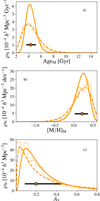 |
Fig. A.1. Histograms of stellar-population parameters (thin line, derived using BC03 SSP models) of the 1480 quiescent galaxies with stellar mass 10.8 ≤ log10 M⋆ < 11.2 dex and at redshift 0.5 ≤ z < 0.7. From top to bottom, mass-weighted age, mass-weighted metallicity, and extinction (panels a, b, and c, respectively). The dashed line is the distribution fit, whereas the solid orange line is the parameter distributions after applying the MLE method to deconvolve uncertainty effects (further details in the text). The star-shaped marker and the solid black line illustrate the median and the 1σ width of the distributions, respectively. All the curves were normalised to the fitted number density (see Sect. 3 and Table 2). |
As we explored potential systematics on stellar population properties due to the use of different population synthesis models, we performed the MLE deconvolution of uncertainty effects on the distributions of age, metallicity, and extinction for BC03 and EMILES (including both BaSTI and Padova00 isochrones) SSP models. In addition, we provided uncertainties for μ(z) and σint(z), making use of the EMCEE Markov chains. The formation epoch, age, metallicity, and extinction PDFs for the ALHAMBRA quiescent galaxies are presented in Appendices A.1–A.3 for BC03, EMILES+BaSTI isochrones, and EMILES+Padova00 isochrones SSP models, respectively. For the analysis of these distributions, we refer readers to Sect. 4.
A.1. Stellar-population PDFs of ALHAMBRA quiescent galaxies: BC03 SSP models
For BC03 SSP models, we adopted a linear dependence of μ(z) and σint(z) for ages and extinctions (i.e. μ2 = σ2 = 0) and a quadratic one for metallicity. It should be noted that we provided the PDFs of stellar population properties at different stellar mass ranges because these properties may depend on stellar mass in a general case. Only for the mass bin 10.0 ≤ log10 M⋆ < 10.4 and for metallicity, we adopted σ2 = 0 because σint(z) is properly reproduced by a linear function and this reduces degeneracy effects during the maximisation of Eq. (A.1). In addition, we compared the μ(z) and σint(z) curves (obtained after carrying out the MLE method) with the values obtained from the same analysis in redshift bins of Δz = 0.2 and setting μ2 = μ1 = σ2 = σ1 = 0 (i.e. the average value of μ(z) and σint(z) at the previously stated redshift bin). As a result, we obtain that the linear and quadratic assumptions are fairly suitable in each case. All the parameters and uncertainties obtained after the maximisation of Eq. (A.1) that are necessary to build the stellar population PDFs are provided in Tables A.1–A.6 (see also Eqs. (A.2)–(A.4)). Notice that the parameters to compute the age and formation epoch PDFs in the log-space are also provided in Tables A.2 and A.4. Co-moving number densities for the PDF normalisation can be found in Table 2 (details in Sect. 3). It is worth mentioning that at z ≳ 1.1, the reliability of the parameters may be questionable. Indeed, we cannot confirm whether μ(z) and σint(z) feature linear or quadratic functional forms with redshift.
Parameters μ(z, M⋆) and σint(z, M⋆) of probability distribution functions of luminosity and mass-weighted ages in real space (Gyr units, see Eq. (A.2)).
Same as Table A.1, but for probability distribution functions of luminosity and mass-weighted age in log-space (age in yr units).
Same as Table A.1, but for probability distribution functions of luminosity and mass-weighted formation epochs in real-space (Gyr units, see Eq. (A.2)).
Same as Table A.1, but for probability distribution functions of luminosity and mass-weighted formation epochs in log-space (age in yr units).
Same as Table A.1, but for probability distribution functions of luminosity and mass-weighted metallicities (see Eq. (A.3)).
Same as Table A.1, but for probability distribution functions of extinctions (see Eq. (A.4)).
Owing to the low number of galaxies at 9.6 ≤ log10 M⋆ < 10.0 and 0.1 ≤ z < 0.3, the MLE deconvolution of uncertainty effects is highly uncertain and degenerated. Only at this mass range, we assume that the median and intrinsic dispersion of the PDFs is constant across cosmic time (μ2 = μ1 = σ2 = σ1 = 0; see Figs. 4–6). Regarding extinction at 0.1 ≤ z < 0.2 and log10 M⋆ ≥ 11.2, we find that the assumption of linearity for σint(z) is not physically (σint ∼ 0.0 at z ∼ 0.1), but only mathematically motivated. Consequently, we adopted a constant value of σint(0.1 ≤ z < 0.2)=σint(z = 0.2) = 0.14 ± 0.03 and μ(0.1 ≤ z < 0.2)=μ(z = 0.2)= − 1.30 ± 0.07 only for quiescent galaxies at 0.1 ≤ z < 0.2 and log10 M⋆ ≥ 11.2. We note that for the lowest extinction values in Eq. (A.4) (AV ∼ 0), the probability might be underestimated because the log-normal function falls to zero at this regime of values.
A.2. Stellar-population PDFs of ALHAMBRA quiescent galaxies: EMILES and BaSTI isochrones
For EMILES SSP models and BaSTI isochrones, we find qualitatively similar trends to those obtained in Appendix A.1. However as expected, there is a quantitative systematic caused by the differing model prescriptions between both model sets. For age, formation epoch, and extinction distributions, a linear dependence with redshift is adopted for μ(z) and σint(z) instead, that is μ2 = σ2 = 0. As in Appendix A.1, the assumption of linearity for μ(z) and σint(z) is supported after comparing with the MLE solutions when values of μ2 = μ1 = σ2 = σ1 = 0 are adopted at redshift bins of Δz = 0.2 (see Fig. 4). Nevertheless, the assumption of a quadratic form for μ(z) and σint(z) is not needed for metallicity and we assumed a linear dependence with redshift for these parameters. The parameters and uncertainties obtained after deconvolving the stellar population distributions provided by MUFFIT using EMILES+BaSTI isochrones to build the stellar population PDFs (Eqs. (A.2)–(A.4)) of quiescent galaxies are provided in Tables A.1–A.6. As in Sect. A.1, for quiescent galaxies at 9.7 ≤ log10 M⋆ < 10.1 we performed the MLE deconvolution of uncertainty effects adopting a constant value for μ(z) and σint(z) at 0.1 ≤ z ≤ 0.3.
A.3. Stellar-population PDFs of ALHAMBRA quiescent galaxies: EMILES and Padova00 isochrones
For Padova00 isochrones, we only appreciated mild quantitative discrepancies with respect the BaSTI ones. As in Appendix A.2, we assumed a linear dependence for μ(z) and σint(z) for all the stellar-population parameters during the MLE process. The values to compute μ(z) and σint(z) along with their uncertainties, meaning the PDFs of age, metallicity, and extinction of quiescent galaxies, are shown in Tables A.1–A.6. For those quiescent galaxies with stellar mass at 9.7 ≤ log10 M⋆ < 10.1 (restricted for completeness reasons at 0.1 ≤ z ≤ 0.3), we provide reference values for its stellar population PDFs assuming μ2 = μ1 = σ2 = σ1 = 0 (for further details, see Sect. 4 and Figs. 4–6).
All Tables
Logarithm of the number density, log10 ρN[h3 Mpc−3], for the quiescent galaxies in our sample as a function of stellar mass and redshift.
Brief description of previous studies trying to constrain stellar population parameters of quiescent galaxies at intermediate redshift.
Parameters μ(z, M⋆) and σint(z, M⋆) of probability distribution functions of luminosity and mass-weighted ages in real space (Gyr units, see Eq. (A.2)).
Same as Table A.1, but for probability distribution functions of luminosity and mass-weighted age in log-space (age in yr units).
Same as Table A.1, but for probability distribution functions of luminosity and mass-weighted formation epochs in real-space (Gyr units, see Eq. (A.2)).
Same as Table A.1, but for probability distribution functions of luminosity and mass-weighted formation epochs in log-space (age in yr units).
Same as Table A.1, but for probability distribution functions of luminosity and mass-weighted metallicities (see Eq. (A.3)).
Same as Table A.1, but for probability distribution functions of extinctions (see Eq. (A.4)).
All Figures
|
Fig. 1. Evolution of number density (Y-axis) of quiescent galaxies in ALHAMBRA with redshift (X-axis), for different stellar mass bins (see inner-panels). Coloured dots illustrate number densities when using a 1/Vmax formalism, whereas solid lines show the best fit to Eq. (1). From top to bottom, number densities obtained from BC03, EMILES+BaSTI, and EMILES+Padova00 SSP models (panels a, b, and c, respectively). Over-plotted, we show the evolution on the number density of massive quiescent galaxies, log10 M⋆ ≥ 11, with redshift from the previous work of Pozzetti et al. (2010, dashed line), Moresco et al. (2013, dotted line), and Moustakas et al. (2013, dash-dot line). In all cases, the number densities at the 0.5 < z < 0.7 bin are excluded from the fit as explained in the text. |
| In the text | |
|
Fig. 2. Photometric-redshift distributions of quiescent (left panel) and star-forming (right panel) galaxies from the ALHAMBRA Gold catalogue down to 0.1 ≤ z ≤ 1.5. Distributions were obtained using the codes BPZ2.0, EAZY, and LePHARE (references in text). To guide the eye, the grey area encloses the redshift bin 0.5 ≤ z ≤ 0.7. |
| In the text | |
|
Fig. 3. Typical uncertainties of stellar population parameters of ALHAMBRA quiescent galaxies. From top to bottom, median of age, metallicity, and extinction uncertainties (panels a, b, and c, respectively) at different redshifts and stellar mass bins (see inner panel). Vertical bars enclose the 68% confidence level of the distribution of uncertainty values. |
| In the text | |
|
Fig. 4. Evolution of mass-weighted age and formation epoch PDFs of quiescent population along cosmic time for different stellar mass bins. Panels a–c and panels d–f: illustrate the evolution of the medians of mass-weighted age and formation epoch PDFs, respectively, whereas panels g–i show the widths of the mass-weighted age PDFs. From left to right, results obtained using the SSP models of BC03 (panels a, d, and g), EMILES with BaSTI isochrones (panels b, e, and h), and EMILES with the Padova00 ones (panels c, f, and i). The shaded regions enclose the 1σ uncertainties of both parameters. The grey region limits the age of the Universe at any redshift. The square-shaped markers illustrate the average median and width assuming for the MLE deconvolution μ2 = μ1 = σ2 = σ1 = 0. |
| In the text | |
|
Fig. 5. Evolution of mass-weighted metallicity PDFs of quiescent population along cosmic time for different stellar mass bins. Panels a–c: illustrate the evolution of the medians of mass-weighted metallicity PDFs, whereas panels g–i show the widths of the mass-weighted metallicity PDFs. From left to right, results obtained using the SSP models of BC03 (panels a and d), EMILES with BaSTI isochrones (panels b and e), and EMILES with the Padova00 ones (panels c and f). The shaded regions enclose the 1σ uncertainties of both parameters. The grey region limits the age of the Universe at any redshift. The square-shaped markers illustrate the average median and width assuming for the MLE deconvolution μ2 = μ1 = σ2 = σ1 = 0. |
| In the text | |
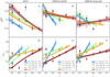 |
Fig. 6. Same as Fig. 5, but for the extinction PDFs of quiescent galaxies. |
| In the text | |
|
Fig. 7. Comparison of ages (panels a, b, and c) and metallicities (panels d, e, and f) of quiescent galaxies from several previous studies and our results from ALHAMBRA at redshift range 0 < z < 1.2. From left to right, the median mass-weighted ages and metallicities retrieved using MUFFIT (solid lines) and BC03 (panels a and d), EMILES with BaSTI (panels b and e), and Padova00 isochrones (panels c and f), respectively. The ages and metallicities retrieved from other work are colour-coded in concordance with their proximity to the stellar mass bins of our quiescent sample (see inset). Dashed orange lines illustrate the average age and metallicity in galaxy clusters obtained by Jørgensen et al. (2017). The grey region limits the Universe age. |
| In the text | |
|
Fig. A.1. Histograms of stellar-population parameters (thin line, derived using BC03 SSP models) of the 1480 quiescent galaxies with stellar mass 10.8 ≤ log10 M⋆ < 11.2 dex and at redshift 0.5 ≤ z < 0.7. From top to bottom, mass-weighted age, mass-weighted metallicity, and extinction (panels a, b, and c, respectively). The dashed line is the distribution fit, whereas the solid orange line is the parameter distributions after applying the MLE method to deconvolve uncertainty effects (further details in the text). The star-shaped marker and the solid black line illustrate the median and the 1σ width of the distributions, respectively. All the curves were normalised to the fitted number density (see Sect. 3 and Table 2). |
| In the text | |
Current usage metrics show cumulative count of Article Views (full-text article views including HTML views, PDF and ePub downloads, according to the available data) and Abstracts Views on Vision4Press platform.
Data correspond to usage on the plateform after 2015. The current usage metrics is available 48-96 hours after online publication and is updated daily on week days.
Initial download of the metrics may take a while.