| Issue |
A&A
Volume 631, November 2019
|
|
|---|---|---|
| Article Number | C2 | |
| Number of page(s) | 6 | |
| Section | Extragalactic astronomy | |
| DOI | https://doi.org/10.1051/0004-6361/201732442e | |
| Published online | 14 November 2019 | |
The ALMA Frontier Fields Survey
IV. Lensing-corrected 1.1 mm number counts in Abell 2744, MACS J0416.1−2403, and MACS J1149.5+2223 (Corrigendum)
1
Instituto de Física y Astronomía, Universidad de Valparaíso, Av. Gran Bretaña 1111, Valparaíso, Chile
e-mail: This email address is being protected from spambots. You need JavaScript enabled to view it.
2
Instituto de Astrofísica y Centro de Astroingeniería, Facultad de Física, Pontificia Universidad Católica de Chile, Casilla 306, Santiago 22, Chile
3
Núcleo de Astronomía de la Facultad de Ingeniería y Ciencias, Universidad Diego Portales, Av. Ejército 441, Santiago, Chile
4
Millennium Institute of Astrophysics, Chile
5
Space Science Institute, 4750 Walnut Street, Suite 205, Boulder, CO 80301, USA
6
Zentrum für Astronomie, Institut für Theoretische Astrophysik, Philosophenweg 12, 69120 Heidelberg, Germany
7
Department of Physics and Astronomy, University College London, Gower Street, London WC1E 6BT, UK
8
Departamento de Ciencias Físicas, Universidad Andres Bello, Av. República 252, Santiago, Chile
9
Leiden Observatory, Leiden University, 2300 Leiden, The Netherlands
10
Department of Astronomy, Universidad de Concepción, Casilla 160-C, Concepción, Chile
11
Carnegie Institution for Science, Las Campanas Observatory, Casilla 601, Colina El Pino s/n, La Serena, Chile
12
Joint ALMA Observatory, Alonso de Córdova 3107, Vitacura, Santiago, Chile
13
European Southern Observatory, Alonso de Córdova 3107, Vitacura, Casilla 19001, Santiago, Chile
14
Chinese Academy of Sciences South America Center for Astronomy, National Astronomical Observatories, CAS, Beijing 100101, PR China
15
Universidad Autónoma de Chile, Chile. Av. Pedro de Valdivia 425, Santiago, Chile
16
Physics Department, Ben-Gurion University of the Negev, PO Box 653, Be’er-Sheva 8410501, Israel
Key words: gravitational lensing: strong / galaxies: high-redshift / submillimeter: galaxies / errata, addenda
We noticed an error in the code that conducts the source injection simulations used in our article Muñoz Arancibia et al. (2018). This error led the source scale radii in the image plane to be 1/2.35 times smaller that what it should be. Wrongly computed scale radii primarily affect the calculation of first, completeness as a function of image-plane integrated flux density curves for different image-plane scale radii; and second, image-plane integrated flux densities estimated for low-significance ALMA detections. These in turn affect the calculation of deboosting correction factors, demagnified integrated flux densities (for low-significance ALMA detections), differential and cumulative number counts, and the contribution to the extragalactic background light.
This error has some effect upon the conclusions of the original manuscript. Figures 1, 2, 5, 6, 9, 11–14, and Table 3 are affected in the original manuscript and are corrected in this erratum. Values in the text should be updated accordingly, as shown in the sentences as follows.
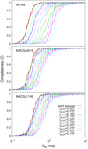 |
Fig. 1. Completeness correction C as function of image-plane integrated flux density and separated in bins of image-plane scale radius. Error bars indicate binomial confidence intervals. |
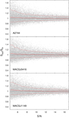 |
Fig. 2. Deboosting correction as function of S/N. We display the ratio between the extracted and injected flux densities for our simulated sources as gray dots. Thick red lines correspond to median values while thin red lines indicate the 16th and 84th percentiles. |
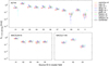 |
Fig. 5. Median demagnified integrated flux density per source for lens models listed in Table 2 (colored symbols), and also combining all models for each cluster field (large black circles). Error bars indicate the 16th and 84th percentiles. Values for each model have been offset around the source ID for clarity. |
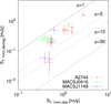 |
Fig. 6. Median demagnified integrated flux density as function of observed integrated flux density for A2744 (red crosses), MACS J0416 (green squares), and MACS J1149 (blue diamonds). Median values were obtained by combining all models for each cluster field. Error bars in demagnified fluxes correspond to the 16th and 84th percentiles, while for observed fluxes, there are 1σ statistical uncertainties. As a reference, black lines indicate magnification values of one (solid), five (dotted), ten (dashed), and 50 (dot-dashed). |
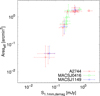 |
Fig. 9. Median effective area as function of demagnified integrated flux density for A2744 (red crosses), MACS J0416 (green squares), and MACS J1149 (blue diamonds). Median values are obtained combining all models for each cluster field. Error bars correspond to the 16th and 84th percentiles. For comparing uncertainty values, both axes cover the same interval in order of magnitude. Within the errors, both demagnified flux densities and effective areas span around 2.5 orders of magnitude. |
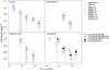 |
Fig. 11. Demagnified differential counts at 1.1 mm, for each cluster (see legends at top-left) and combining all cluster fields (bottom-right panel). Values correspond to median counts for the lens models listed in Table 2 (colored symbols), combining all models for each cluster field (large black crosses, squares, and diamonds) and combining all models for all cluster fields (large black filled circles). Error bars indicate the 16th and 84th percentiles, adding the scaled Poisson confidence levels for 1σ lower and upper limits respectively in quadrature. Arrows indicate 3σ upper limits for flux density bins that have zero median counts and non-zero values at the 84th percentile. In the first three panels, counts for each model have been offset in flux around the combined counts for clarity. In the bottom-right panel, this is done for each galaxy cluster field around the counts that combine all models for all cluster fields. |
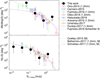 |
Fig. 13. Differential (top) and cumulative (bottom) counts at 1.1 mm compared to ALMA results and galaxy formation model predictions from literature. Our counts (large black filled circles) correspond to median values combining all models for all cluster fields. Error bars indicate the 16th and 84th percentiles, adding the scaled Poisson confidence levels for 1σ lower and upper limits respectively in quadrature. Arrows indicate 3σ upper limits for flux densities having zero median counts and non-zero values at the 84th percentile. We show previous results reported by Ono et al. (2014) as red crosses, Carniani et al. (2015) as blue squares, Fujimoto et al. (2016) as green diamonds (with their Schechter fit shown as a black dashed line), Oteo et al. (2016) as red triangles, Hatsukade et al. (2016) as blue crosses, Aravena et al. (2016) as green squares, Umehata et al. (2017) as red diamonds, and Dunlop et al. (2017) as a black solid curve. We show number counts predicted by the galaxy formation models from Cowley et al. (2015; orange line), Béthermin et al. (2017; cyan line), and Schreiber et al. (2017; magenta line). We scale the counts derived at other wavelengths as S1.1 mm = 1.29 × S1.2 mm and S1.1 mm = 1.48 × S1.3 mm (following Hatsukade et al. 2016). |
Demagnified 1.1 mm number counts.
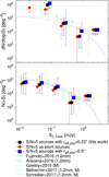 |
Fig. 14. Differential (top) and cumulative (bottom) counts at 1.1 mm for different assumptions regarding image-plane source scale radii for low-significance sources: adopting |


In the Abstract. In combining all cluster fields, our number counts span around two orders of magnitude in demagnified flux density, from several mJy down to tens of μJy. Both of our differential and cumulative number counts are consistent with most of the recent estimates from deep ALMA observations at a 1σ level. Below ≈0.1 mJy, however, our cumulative counts are lower by ≈0.5 dex, suggesting flattening in the number counts.
In Section 2.1.2. From source injection simulations (see Sect. 3.1), we find a typical ratio between the peak and integrated flux density for these size parameters of 0.50, 0.80, and 0.80 in Abell 2744, MACS J0416.1−2403, and MACS J1149.5+2223, respectively (hereafter A2744, MACS J0416, and MACS J1149). By scaling the peak intensities by these ratios, the integrated flux densities of the 4.5 ≤ S/N < 5 detections (with S/N the signal-to-noise ratio) range from ∼0.38 to ∼0.65 mJy.
In Section 3.1. However, the completeness drops to 2%, 10%, and 20% at the same flux densities for image-plane source sizes in the range of  (i.e., for the image-plane size assumed for our low-significance detections).
At S/N = 4.5, we find that the noise boosts the flux densities by 4%, 5%, and 5% for A2744, MACS J0416, and MACS J1149, respectively.
In Section 3.2. We obtain the fraction of spurious sources at a given S/N, pfalse, defined as the average ratio between the number of sources detected over that peak S/N in the simulated noise maps and in the true mosaic. We found this typo in the description after publication of our manuscript.
In Section 3.3. Some sources that have a median of μ ≳ 10 reach dispersions ≳0.5 dex, such as source A2744-ID09 in the Diego v4.1 model. After acceptance of our manuscript, Sharon v4 models in the FF website were corrected; in the updated Sharon v4 model, A2744-ID11 has a median μ ≈ 19, reaching a dispersion of only ≈0.2 dex.
In Section 3.4. Median (combined) lensing-corrected flux densities range from ∼0.04 to 1.62 mJy; both the faintest and brightest sources in the sample are found around A2744.
Within the uncertainties, combined demagnified flux densities cover around 2.1 orders of magnitude.
At Sobs ≳ 0.5 mJy, we find a trend of brighter observed sources that are also brighter intrinsically, while sources having lower observed flux densities tend to span ≈1.5 dex in demagnified flux.
We also find that sources with the highest magnifications (μ ≳ 5) are among the faintest ones both in observed and lensing-corrected flux (Sobs ≲ 0.5 mJy and Sdemag ≲ 0.1 mJy, respectively).
In Section 3.5. At ≈0.1−0.3 mJy, sources with a Sdemag 1σ interval of 0.3 dex, for example, have an Aeff 1σ interval close to 0.5 dex. Below 0.1 mJy, uncertainties in both of those quantities remain comparable in terms of order of magnitude, which reaches a 1σ interval of ≲1 dex.
In Section 4.1. Uncertainties coming from our Monte Carlo simulation (i.e., using the whole probability distributions for observed flux densities, source redshifts, and magnifications together) differ by a factor of ∼0.03−4.62 from what was predicted from Poisson statistics.
We present counts down to the flux density where at least one cluster field has non-zero combined differential counts at the 84th percentile, that is, centered on 0.024 mJy. Combining all cluster fields, our differential counts eventually span ∼2 orders of magnitude in demagnified flux density, going from the mJy level down to tens of μJy. This is ≈1.3 times deeper than the observed rms level reached in our deepest ALMA FF mosaic, A2744.
In these three cases, variations in the median counts that combine all cluster fields are only up to ≈0.08 dex below 1.3 mJy. Our combined counts are also in agreement within the errors with those obtained centering the Gaussian at z = 3 ± 0.5 for all detections (although it adds a 3σ upper limit of ∼106 deg−2 at 0.024 mJy due to the larger high-magnification regions for this redshift).
In Section 4.2. At 0.133–0.422 mJy, our number counts are consistent within 1σ with all but Hatsukade et al. (2016) data.
Also below this flux density, our cumulative counts are lower by ≈0.5 dex than Aravena et al. (2016) data, but they are consistent with their results at a 1σ level.
In Section 4.3. In this case, we obtain the integrated flux densities of the low-significance detections, scaling the peak intensities by the typical ratios 0.18, 0.46, and 0.47 in A2744, MACS J0416, and MACS J1149, respectively.
We find that assuming reff, obs = 0.5″ for low-significance sources maintains the agreement with Aravena et al. (2016) at 1σ. Assuming that our low-significance detections are point sources disagrees with their estimates at 1σ, although this remains consistent with Fujimoto et al. (2016) counts assuming our 3σ upper limit.
Below 0.133 mJy, our fiducial number counts are consistent with available data from both serendipitous and blank-field surveys at a 1σ level.
In Section 4.4. We estimate a median contribution of 
 Jy deg−2 resolved in our demagnified sources at 1.1 mm down to 0.013 (0.133) mJy, with uncertainties computed from the 16th and 84th percentiles.
The contribution provided by our demagnified sources represents 
 of this EBL at 1.1 mm down to 0.013 (0.133) mJy. As expected from Fig. 13, this contribution is lower than the results from Carniani et al. (2015) and Hatsukade et al. (2016), which are both at 1.1 mm. However, this contribution is consistent to ≈1σ with their results.
In Section 5. By combining all cluster fields, our differential number counts span around two orders of magnitude in demagnified flux density, going from the mJy level down to tens of μJy.
Within the error bars in our number counts (coming from both Poisson errors and lensing model uncertainties) our results are consistent at 1σ with most of the recent estimates from deep ALMA observations (Ono et al. 2014; Carniani et al. 2015; Fujimoto et al. 2016; Oteo et al. 2016; Hatsukade et al. 2016; Aravena et al. 2016; Umehata et al. 2017; Dunlop et al. 2017). However, below ≈0.1 mJy, our cumulative number counts are ≈0.5 dex lower than previous estimates.
References
- Aravena, M., Decarli, R., Walter, F., et al. 2016, ApJ, 833, 68 [NASA ADS] [CrossRef] [Google Scholar]
- Béthermin, M., Wu, H.-Y., Lagache, G., et al. 2017, A&A, 607, A89 [NASA ADS] [CrossRef] [EDP Sciences] [Google Scholar]
- Carniani, S., Maiolino, R., De Zotti, G., et al. 2015, A&A, 584, A78 [NASA ADS] [CrossRef] [EDP Sciences] [Google Scholar]
- Cowley, W. I., Lacey, C. G., Baugh, C. M., & Cole, S. 2015, MNRAS, 446, 1784 [NASA ADS] [CrossRef] [Google Scholar]
- Dunlop, J. S., McLure, R. J., Biggs, A. D., et al. 2017, MNRAS, 466, 861 [NASA ADS] [CrossRef] [Google Scholar]
- Fujimoto, S., Ouchi, M., Ono, Y., et al. 2016, ApJS, 222, 1 [NASA ADS] [CrossRef] [Google Scholar]
- Hatsukade, B., Kohno, K., Umehata, H., et al. 2016, PASJ, 68, 36 [NASA ADS] [CrossRef] [Google Scholar]
- Muñoz Arancibia, A. M., González-López, J., Ibar, E., et al. 2018, A&A, 620, A125 [NASA ADS] [CrossRef] [EDP Sciences] [Google Scholar]
- Ono, Y., Ouchi, M., Kurono, Y., & Momose, R. 2014, ApJ, 795, 5 [NASA ADS] [CrossRef] [Google Scholar]
- Oteo, I., Zwaan, M. A., Ivison, R. J., Smail, I., & Biggs, A. D. 2016, ApJ, 822, 36 [NASA ADS] [CrossRef] [Google Scholar]
- Schreiber, C., Elbaz, D., Pannella, M., et al. 2017, A&A, 602, A96 [NASA ADS] [CrossRef] [EDP Sciences] [Google Scholar]
- Umehata, H., Tamura, Y., Kohno, K., et al. 2017, ApJ, 835, 98 [NASA ADS] [CrossRef] [Google Scholar]
© ESO 2019
All Tables
All Figures
|
Fig. 1. Completeness correction C as function of image-plane integrated flux density and separated in bins of image-plane scale radius. Error bars indicate binomial confidence intervals. |
| In the text | |
|
Fig. 2. Deboosting correction as function of S/N. We display the ratio between the extracted and injected flux densities for our simulated sources as gray dots. Thick red lines correspond to median values while thin red lines indicate the 16th and 84th percentiles. |
| In the text | |
|
Fig. 5. Median demagnified integrated flux density per source for lens models listed in Table 2 (colored symbols), and also combining all models for each cluster field (large black circles). Error bars indicate the 16th and 84th percentiles. Values for each model have been offset around the source ID for clarity. |
| In the text | |
|
Fig. 6. Median demagnified integrated flux density as function of observed integrated flux density for A2744 (red crosses), MACS J0416 (green squares), and MACS J1149 (blue diamonds). Median values were obtained by combining all models for each cluster field. Error bars in demagnified fluxes correspond to the 16th and 84th percentiles, while for observed fluxes, there are 1σ statistical uncertainties. As a reference, black lines indicate magnification values of one (solid), five (dotted), ten (dashed), and 50 (dot-dashed). |
| In the text | |
|
Fig. 9. Median effective area as function of demagnified integrated flux density for A2744 (red crosses), MACS J0416 (green squares), and MACS J1149 (blue diamonds). Median values are obtained combining all models for each cluster field. Error bars correspond to the 16th and 84th percentiles. For comparing uncertainty values, both axes cover the same interval in order of magnitude. Within the errors, both demagnified flux densities and effective areas span around 2.5 orders of magnitude. |
| In the text | |
|
Fig. 11. Demagnified differential counts at 1.1 mm, for each cluster (see legends at top-left) and combining all cluster fields (bottom-right panel). Values correspond to median counts for the lens models listed in Table 2 (colored symbols), combining all models for each cluster field (large black crosses, squares, and diamonds) and combining all models for all cluster fields (large black filled circles). Error bars indicate the 16th and 84th percentiles, adding the scaled Poisson confidence levels for 1σ lower and upper limits respectively in quadrature. Arrows indicate 3σ upper limits for flux density bins that have zero median counts and non-zero values at the 84th percentile. In the first three panels, counts for each model have been offset in flux around the combined counts for clarity. In the bottom-right panel, this is done for each galaxy cluster field around the counts that combine all models for all cluster fields. |
| In the text | |
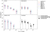 |
Fig. 12. As in Fig. 11, but for demagnified cumulative number counts at 1.1 mm. |
| In the text | |
|
Fig. 13. Differential (top) and cumulative (bottom) counts at 1.1 mm compared to ALMA results and galaxy formation model predictions from literature. Our counts (large black filled circles) correspond to median values combining all models for all cluster fields. Error bars indicate the 16th and 84th percentiles, adding the scaled Poisson confidence levels for 1σ lower and upper limits respectively in quadrature. Arrows indicate 3σ upper limits for flux densities having zero median counts and non-zero values at the 84th percentile. We show previous results reported by Ono et al. (2014) as red crosses, Carniani et al. (2015) as blue squares, Fujimoto et al. (2016) as green diamonds (with their Schechter fit shown as a black dashed line), Oteo et al. (2016) as red triangles, Hatsukade et al. (2016) as blue crosses, Aravena et al. (2016) as green squares, Umehata et al. (2017) as red diamonds, and Dunlop et al. (2017) as a black solid curve. We show number counts predicted by the galaxy formation models from Cowley et al. (2015; orange line), Béthermin et al. (2017; cyan line), and Schreiber et al. (2017; magenta line). We scale the counts derived at other wavelengths as S1.1 mm = 1.29 × S1.2 mm and S1.1 mm = 1.48 × S1.3 mm (following Hatsukade et al. 2016). |
| In the text | |
|
Fig. 14. Differential (top) and cumulative (bottom) counts at 1.1 mm for different assumptions regarding image-plane source scale radii for low-significance sources: adopting |
| In the text | |
Current usage metrics show cumulative count of Article Views (full-text article views including HTML views, PDF and ePub downloads, according to the available data) and Abstracts Views on Vision4Press platform.
Data correspond to usage on the plateform after 2015. The current usage metrics is available 48-96 hours after online publication and is updated daily on week days.
Initial download of the metrics may take a while.